| Issue |
A&A
Volume 700, August 2025
|
|
|---|---|---|
| Article Number | A80 | |
| Number of page(s) | 17 | |
| Section | Stellar atmospheres | |
| DOI | https://doi.org/10.1051/0004-6361/202555181 | |
| Published online | 07 August 2025 | |
Spectral analysis of HD 49798, a bright, hydrogen-deficient sdO-type donor star in an accreting X-ray binary
Institute for Astronomy and Astrophysics, Kepler Center for Astro and Particle Physics, Eberhard Karls University,
Sand 1,
72076
Tübingen,
Germany
★ Corresponding author: This email address is being protected from spambots. You need JavaScript enabled to view it.
Received:
16
April
2025
Accepted:
25
June
2025
Abstract
Context. HD 49798 is a bright (mV = 8.287), hot (effective temperature Teff = 45 000 K) subdwarf star of the spectral type O (sdO). It is the only confirmed sdO-type mass-donor star of an X-ray binary that has a high-mass (1.28 M☉) white-dwarf or neutron-star primary with a spin period of only 13.2 s.
Aims. Since a high-quality spectrum of HD 49798, obtained with the Tübingen Ultraviolet Echelle Spectrometer (TUES), that has never been analyzed before is available in the database of the Orbiting and Retrievable Far and Extreme Ultraviolet Spectrometer (ORFEUS), we performed a spectral analysis based on observations from the far ultraviolet (FUV) to the optical wavelength range.
Methods. We used advanced non-local thermodynamic equilibrium (NLTE) model atmospheres of the Tübingen Model-Atmosphere Package (TMAP) to determine the effective temperature, the surface gravity (log g), and the abundances of those elements that exhibit lines in the available observed spectra.
Results. We determined Teff = 45 000 ± 1000 K, log g = 4.46 ± 0.10, and re-analyzed the previously determined photospheric abundances of H, He, N, O, Mg, Al, Si, Fe, and Ni. For the first time, we measured the abundances of C, Ne, P, S, Cr, and Mn.
Conclusions. Our panchromatic spectral analysis of HD 49798 – from the FUV to the optical – allowed us to reduce the error limits of the photospheric parameters and to precisely measure the metal abundances. HD 49798 is a stripped, intermediate-mass (zero-age main sequence mass of MZAMS ≈ 7.15 M☉) He star with a mass of 1.14−0.24+0.30 M⊙. At its surface, it exhibits abundances that are the result of CNO-cycle and 3 α burning nucleosynthesis as well as enhanced Cr, Mn, Fe, and Ni abundances.
Key words: stars: abundances / stars: atmospheres / stars: individual: HD49798 / subdwarfs / X-rays: binaries / X-rays: individuals: RXJ0648.0-4418
© The Authors 2025
 Open Access article, published by EDP Sciences, under the terms of the Creative Commons Attribution License (https://creativecommons.org/licenses/by/4.0), which permits unrestricted use, distribution, and reproduction in any medium, provided the original work is properly cited.
This article is published in open access under the Subscribe to Open model. This email address is being protected from spambots. You need JavaScript enabled to view it. to support open access publication.
1 Introduction
HD 49798 is located in the constellation Puppis and was first mentioned in the Henry Draper Catalogue (Cannon & Pickering 1918) as an Oe5-type with Ptm and Ptg brightnesses of 8.6 and 7.6, respectively. It exhibits a very strong ζ Puppis series of He II lines. It was then observed by Oosterhoff (1951), who found a photo-electric magnitude of m = 8.23 in the yellow spectral region (filter 3385). Landolt & Uomoto (2007) measured brightnesses for stars used as spectrophotometric standards for the Hubble Space Telescope (HST) and found mV = 8.287 for HD 49798 (which was too bright for their original observing plan).
Feast et al. (1957) identified a very strong He II Pickering series and a variable velocity. Jaschek & Jaschek (1963) analyzed optical spectra and reported then on the discovery of a new O-type subdwarf (sdO), which was the brightest known at that time and – even more important – in a spectroscopic binary.
By comparing the spectra of H I, He I, and He II dominated helium-rich hot subdwarfs, Jeffery et al. (1997) proposed a classification scheme (Fig. 1) to further differentiate between different types of sdOs.
HD 49798 is difficult to place in this scheme, as it deviates from the typical spectral features described by Heber (2016). He I λ 4471 Å and He II λ 4543 Å are slightly shallower than H γ. This makes the sdOX:He2 classification the only reasonable one although the features of the spectrum are not described perfectly. The line-depth relation of He II λ 4686 Å>He I λ 4471 Å gives a final classification of sdO5:He2.
A first quantitative analysis of HD 49798 was presented by Richter (1971), who used a local thermodynamical equilibrium (LTE) approach with flux-constant, unblanketed models to fit the observed lines. He found an effective temperature of Teff = 45 000 K, a surface gravity of log (g/cm/s2)=5, log ϵHe = 11.8, and log ϵH = 9.7 (relative to log ϵ☉ = 12, i.e., a number ratio NHe/NH = 0.63). He estimated a stellar mass of M = 2 M☉. Dufton (1972) used optical spectra and investigated non-LTE (NLTE) effects. He arrived at Teff = 45 000 ± 5000 K, log g = 4.3 ± 0.3, and a He overabundance of five. Kudritzki (1976) calculated a grid of H+He composed NLTE model atmospheres and derived Teff = 43 700 K, log g = 4.1 and Teff = 38 000 K, log g = 4.3 for the two grid abundances NHe/NH = 0.1 and NHe/NH = 1.0, respectively. This was refined in an individual complete NLTE analysis by Kudritzki & Simon (1978) with H+He models. They measured Teff = 47 500 ± 2000 K, log g = 4.25 ± 0.2 and  .
.
From the P Cygni line profile of the N V resonance line (cf. Fig. 2) in a spectrum obtained with the International Ultraviolet Explorer (IUE), Hamann et al. (1981) determined a mass-loss rate of −9.3 ≲(Ṁ/M☉/yr) ≲ 8.0 and a terminal wind velocity of v∞ = 1350 km/s.
HD 49798 is the sdO donor in a binary system (orbital period P ≈ 1.55 d, Thackeray 1970) for a pulsating X-ray source (RX J0648.0–4418, M ≈ 1.2 M☉). It may be either a massive white dwarf (WD) or a neutron star (Mereghetti et al. 2009).
To constrain the previous and future evolution of this system and to determine the nature of HD 49798’s companion, Brooks et al. (2017) performed various MESA1 simulations. They used Teff = 47 500 K of Kudritzki & Simon (1978) for their calculations. Two scenarios for the origin of sdOs in binaries are most likely. One, in which the companion is a neutron star, is a core-collapse supernova of a star with a zero-age main sequence (ZAMS) mass ≳ 10 M☉. A detailed description can be found in Branch & Wheeler (2017), Nomoto (1987), e.g., stars with ZAMS masses of 8-10 M☉ undergo He and C burning, which leaves behind a non-degenerate O+Ne+Mg core, light enough that no Ne burning occurs. The subsequent evolution consists of a H-He double-shell burning. As soon as the core (including the C+O layer) reaches the critical mass of 1.375 M☉, electron capture on 20F, 20Ne, 24Na, and 24Mg takes place that induces a rapid contraction of the core. The outward traveling shock due to the bounce-back of the shell on to the core gives rise to the supernova explosion, leaving behind a neutron star.
An sdO scenario that also fits the observations consists of a 7.15 M☉ ZAMS star that enters a common envelope (CE) with its compact companion just before the second dredge-up on the early asymptotic giant branch. These simulations hold for both types of compact companions as the evolution of HD 49798 in this scenario is the same up until the Roche-lobe overflow (RLOF) and is similar afterwards.
The X-ray spectrum and the nature of the compact companion star were the focus of several studies (Mereghetti et al. 2009, 2011, 2013, 2021; Rigoselli et al. 2023) and strongly improved our evolutionary picture. Brooks et al. (2017) investigated its past binary interaction and estimated a time of 65 000 yr from now for the HD 49798 to fill its Roche lobe. Then the companion will accrete at a rate of about 10−5 M☉/yr. Recently, Krtička et al. (2019) analyzed new optical spectra obtained with the Ultraviolet and Visual Echelle Spectrograph (UVES) of the European Southern Observatory (ESO). In addition, they used spectra taken with the Goddard High-Resolution Spectrograph (GHRS) that had been aboard the HST. They derived Teff = 45 900 ± 800 K, M = 1.46 ± 0.32 M☉, and determined the photospheric abundances of H, He, N, O, Mg, Al, Si, Fe, and Ni. Since the Orbiting and Retrievable Far and Extreme UV Spectrometer (ORFEUS) spectrum of HD 49798, obtained with the Tübingen Ultraviolet Echelle Spectrometer (TUES), had been neglected, we decided to perform a detailed spectral analysis with advanced NLTE model-atmosphere techniques.
In Sect. 2, we briefly describe the observations, followed by an overview of the atomic data used and our NLTE model-atmosphere code in Sect. 3. The analysis is presented in Sect. 4. We summarize our results and conclude in Sect. 6.
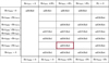 |
Fig. 1 Classification scheme for hot subdwarf stars by Jeffery et al. (1997). The red box denotes the classification of HD 49798. |
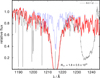 |
Fig. 2 Section of the TUES observation around Ly α (black). The interstellar H I absorption was calculated with NH I = 1.8 (full, red) ± 0.5 (dashed, red, 2.5 times the estimated error range for clarity) × 1020 cm−2. The pure stellar spectrum is shown in blue. A rotational line broadening (vrot = 37.5 km/s) is applied. Interstellar metal lines are not modeled in this plot. The P Cygni profile of the N V resonance line is marked at the top. |
2 Observations, interstellar reddening, and line absorption
ORFEUS2 was an ultraviolet (UV) telescope with an 1 m mirror and a high resolving power R = λ/Δ λ ≈ 10 000. On its second flight (Nov. 19-Dec. 7, 1996, the so-called ORFEUS II mission), HD 49798 was observed for 1292 s (ObsId 2255_1, start time Dec 3 1996, 08:04:36 GMT) with the Tübingen Echelle Spectrograph (TUES). The count rate within 904.63 ≤ λ/Å ≤ 1410.45 was 6221.3/s. We used the spectrum (orders 40 to 61) from our institute’s database3. The same data is available at the Barbara A. Mikulski Archive for Space Telescopes (MAST)4.
In addition, we used the same UV observation taken with GHRS aboard the HST and the optical spectrum (3752 ≤ λ/Å ≤ 5000) like Krtička et al. (2019). The latter was obtained with the UVES at the Very Large Telescope (VLT) of the ESO on Oct. 2, 2016. The exposure time was 180 s and a 0.′′6 slit was used. With a resolution-slit product of 41 400, we assume a resolving power of R = λ/Δ λ ≈ 69 000.
A summary of the observed spectra of HD 49798 used in this analysis is given in Table 1. A comparison of the observations shows that the GHRS spectra are significantly lower in their flux level (Fig. 3): the two spectra with λ<1400 Å (Table 1) by a factor of about 1.4, the others by a factor of about 1.8. Most probably, the pipeline flux-calibration procedure went wrong for these six GHRS observations.
In all of our plots, the observations are shifted to rest wavelength. To slightly smooth the UV observations, they are processed with a low-pass filter (Savitzky & Golay 1964).
To determine the interstellar reddening, we applied the reddening law of Fitzpatrick (1999) to our final synthetic stellar spectrum and normalized it to the 2MASS H magnitude. We achieved the best agreement to the UV observations at EB−V = 0.038 within a small error range of 0.010 (Fig. 3).
The interstellar neutral hydrogen column density was measured from a comparison of our theoretical H I Lyman α line profile with the TUES observation. We reproduced the observation best at NH I = 1.8 ± 0.2 × 1020 cm−2 (Fig. 2). This value is in agreement with a reddening value of EB−v = 0.038 ± 0.010 if we consider the empirical relation for the Galactic reddening of Groenewegen & Lamers 1989, log (NHI/EB−V) = 21.58 ± 0.10) and arrive at  .
.
For the detailed calculation of the interstellar line absorption, we used the line-fitting procedure OWENS (Hébrard et al. 2002; Hébrard & Moos 2003). It can model different clouds in the interstellar medium (ISM) with individual radial and turbulent velocities, temperatures, column densities, and chemical compositions. It fits Voigt profiles to the observation using a χ2 minimization.
Observed spectra used in this analysis.
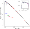 |
Fig. 3 TUES, GHRS, and IUE observations compared with our final model normalized to the 2MASS H magnitude. EB−v = 0.038 ± 0.010 is applied. In addition, the B and V magnitudes (Landolt & Uomoto 2007) as well as the 2MASS J, H, and Ks magnitudes (Cutri et al. 2003) are shown. For clarity, TUES and GHRS spectra are convolved with a Gaussian with a full width at half maximum (FWHM) of 7Å. |
3 Atomic data, model atmospheres, and line broadening
Although prominent P Cygni line profiles of N IV, N V, and S VI are exhibited in the TUES spectrum of HD 49798 (a weak stellar wind was measured by Hamann et al. 1981, Sect. 1), most of the lines are obviously not contaminated by wind effects. Thus, we decided to use the Tübingen NLTE model-atmosphere package (TMAP, Werner et al. 2012) to calculate plane-parallel models in radiative and hydrostatic equilibrium. These consider the opacities of H, He, C, N, O, Ne, Mg, Al, Si, P, S, Ca, Sc, Ti, V, Cr, Mn, Fe, Co, and Ni. Level dissolution (pressure ionization) following Hummer & Mihalas (1988) and Hubeny et al. (1994) is considered.
For elements with an atomic number Z below 20, the atomic data were compiled from our Tübingen Model Atom Database (TMAD, Rauch & Deetjen 2003), which was constructed as part of the Tübingen contribution to the German Astrophysical Virtual Observatory (GAVO). For Z ≥ 20, we used a statistical approach using super levels and super lines (Rauch & Deetjen 2003) and calculated the atomic data via our Iron Opacity and Interface (IrOnIc, Müller-Ringat 2013).
For the detailed line-profile calculations, we used Stark-broadening tables of Tremblay & Bergeron (2009, extended tables of 2015, priv. comm.) and Schöning & Butler (1989) for the H I and He II lines, respectively. Stark line-broadening tables from Barnard et al. (1974,1975) and were used for He I λ λ 4471, 4921 Å, respectively, Griem (1974) for other He I lines, and Dimitrijević & Sahal-Bréchot (1992b,a); Dimitrijevic & Sahal-Brechot (1995); Dimitrijević et al. (1991) were used for C IV, N V, O IV – V, and Si IV lines, respectively.
The sharp metal lines that are broadened due to the quadratic Stark effect show the impact of rotational broadening in their line cores. As an example, we show the prominent N III λ λ 3998.63, 4003.58Å lines of the 4d 2D – 5f2Fo multiplet in Fig. 4. The average determined projected rotational velocity from these and many other lines is vrot = 37.5 ± 5 km/s. This matches the value vrot = 40 ± 5 km/s measured by Krtička et al. (2019).
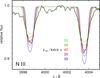 |
Fig. 4 Our final model spectrum with different vrot(30−50 km/s, the labels’ colors refer to the respective spectra) applied, compared with a section of the UVES observation around N III λ λ 3998.63, 4003.58Å. |
4 Analysis
For our first test models, we adopted the parameters of Krtička et al. (2019, Teff = 45 900 K, log g = 4.56), and used the elements (H, He, N, O, Mg, Al, Si, Fe, and Ni) with detailed abundance analysis of Krtička et al. (2019). For C, we used their upper limit. Other elements that were mentioned by Krtička et al. (2019) and included in their models with solar abundance values were neglected here. We used their observed optical spectrum (Fig. 5) for comparison.
Krtička et al. (2019) determined H and He mass fractions of 0.25 and 0.74, respectively, with an uncertainty of ± 10 %. At this H/He abundance ratio, all H I Balmer-series line cores but that of H β are well reproduced with our test model (Fig. 5, with dashed violet lines). With our TMAP models (Teff = 45 000 K, log g = 4.46, see their determinations below), we reproduced the individual line cores of H γ−ζ well at H and He abundances of 0.20 and 0.78 ± 2, respectively (Fig. 5). This is, within error limits, in agreement with the result of Krtička et al. (2019).
The too-shallow line core of H β (Fig.5) in our model is unexplained. A significant impact of the so-called Balmer-line problem (Napiwotzki & Rauch 1994, e.g.,) can be excluded, since we considered many metals in detail (Sect. 3). The Balmer-line problem arises if a too-low metal opacity is considered in the models, e.g., in pure H+He models. In such models. the resulting too-high temperature in the outer atmospheres where the lower members of the Balmer series form (Fig. 6) makes it impossible to reproduce all observed Balmer-line profiles with the same Teff.
We adopted our H/He abundance values of 0.20/0.79 from the H γ−ζ/He II blends. We checked the abundances during our further analysis after any change in the atmospheric parameters.
The effective temperature was determined from ionization equilibria, i.e., by the evaluation of the equivalent-width ratios of lines of at least two subsequent ionization stages – this is a very sensitive indicator for Teff. Thus, we calculated models with different Teff (43 000−49 000 K, Fig. 7). We started with the He I/He II ionization equilibrium and verified this result by other ionization equilibria of metals, where we could even identify lines of three subsequent ionization stages.
While the He II line profiles do not change significantly in our above Teff interval, the He II lines are dependent on Teff. We do not have a perfect agreement at one Teff, but 45 000 ± 1000 K was a good start value for the analysis of the ORFEUS II observation. This is in agreement with the result of Krtička et al. (2019, Teff = 45 900 ± 800 K). Other ionization equilibria were checked in the flow of our analysis to verify this preliminary result and to reduce the error range.
The surface gravity was examined using H I and He II lines within 4.16 ≲ log g ≲ 4.76 (starting with the value of log g = 4.56 ± 0.08 of Krtička et al. 2019). An example of our comparison is shown in Fig. 7. While the line cores are too deep and the line wings are too narrow at the lower values, the central depression of the lines in the observation is not reproduced at the higher values. We adopted log g = 4.46 ± 0.1. This is well in agreement with Krtička et al. (2019).
With our new parameters, we improved the agreement between the synthetic and observed spectra (cf. Fig. 1 of Krtička et al. 2019). From our new models, we calculated spectra for the analysis of the TUES, GHRS, and UVES observations.
In the following, we determine the abundances of C, N, O, Ne, Mg, Al, Si, P, S, Cr, Mn, Fe, and Ni using this strategy. In the case that lines of an element are exhibited in our model, we try to identify their observed counterparts. Since the rotational velocity (vrot = 40 km/s) results in a significant line broadening, wavelengths of lines that contribute to absorption features can be measured from the unrotated synthetic spectrum. In most figures, a thin, light green line shows a synthetic spectrum, which was calculated without the opacities of the respective element. The comparison to the red line, which is a synthetic spectrum that was calculated from the same model considering the opacities of that element, allows us to identify its line-opacity contributions even in blended line features.
Subsequently, we adjusted the model abundances to reproduce the observation well. Table 2 summarizes the strategic lines used in this analysis. With the improved abundances, the model was then recalculated to account for the impact of the changed opacities on the atmospheric structure and verify the metal abundances (as well as Teff, log g, and the other abundance ratios). To determine the abundance uncertainties due to the error propagation from Teff and log g, we measured the abundances from two models at the error limits of Teff and log g, namely the Teff+ Δ Teff/log g−Δ log g and the Teff−Δ Teff/log g+Δ log g models (the Δ s are the error ranges), for the highest- and lowest-ionization models, respectively.
Here, we provide some examples of our abundance analysis. A complete comparison of observations and synthetic spectra, including a detailed modeling of the interstellar line absorption, is shown in Figs. A.1–A.3. A comparison to the abundance determinations of Krtička et al. (2019) is given in Table 4 and Fig. 20. In the following, we use mass fractions for the determined abundances.
The carbon abundance was measured using the prominent C III λ λ 1174.93−1176.37Å and C IV λ λ 1168.89, 1168.98Å. Lines in the optical wavelength range are much shallower and, thus give a higher uncertainty range for the determined abundances. We find a good agreement with the TUES observation at a C mass fraction of  (Fig. 8, for clarity, we show ± 1 dex). In addition, the ionization equilibrium is well matched with our Teff = 45 000 K/log g = 4.46 model (Fig. 8). In the UVES spectrum (Fig. 8, bottom panel), C IV λ λ 4440.33−4441.74Å A, which are generally the strongest C lines in the optical, are not visible.
The nitrogen abundance cannot be determined precisely from a comparison of the TUES observation and synthetic spectra. Although N III and N IV lines are prominent in the observation and are sufficiently well reproduced by our models, their line cores appear to be almost saturated (Fig. 9). The line wings of N IV λ 954.47Å are more dependent on the N abundance than those of the N III lines. An indicator for the N abundance is the red wing of N IV λ 954.47Å, which is blended by a strong Fe V line. The center of gravity of this line is visible in the wing and well modeled at an N abundance of  (Fig. 9, we show ± 0.4 dex). At this abundance, the optical observation is very well reproduced (Fig. 10).
The oxygen abundance is determined from the most prominent O III lines in the UVES observation, namely О III λ λ 3757.23, 3759.88 Å (Fig. 11). We measure an O abundance of  .
.
The iron-group abundances (here the abundances of calcium to nickel) have a strong impact on the atmospheric structure. Since at first glance an inspection of our UV observations revealed a high number of iron and nickel lines, we started with an abundance analysis of these two elements to include their opacities in our model-atmosphere calculations. The abundances of Ca, Sc, Ti, V, Mn, Cr, and Co are then, in the first step of our calculations, scaled to the Fe abundance with the solar abundance pattern to model their contribution to the background opacity. In the course of this analysis, we use then the newly determined values, where available.
The iron abundance of  turned out to be significantly higher (about three to seven times in the error range) than the solar abundance (Scott et al. 2015a, 1.3 × 10⁻³). Since there are so many Fe lines in the UV wavelength region, we show some representatives in Fig. 12.
The nickel abundance is also derived from many Ni lines in the UV, we show some examples in Fig. 13. The determined Ni abundance is  . This is, like found for Fe, also much higher (five to eleven times) than the solar value of 7.6 × 10⁻⁵ (Scott et al. 2015a). The Fe/Ni mass-fraction ratio is
  , which is lower than the solar ratio of 16.9, but agrees within its error limits.
The neon abundance determination uses Ne II and Ne III lines (Fig. 14) that are identified in the UVES spectrum. We find a Ne abundance of  .
.
The magnesium abundance is measured from the most prominent magnesium line, namely Mg II λ 4481.143 Å (Fig. 15). We arrive at a Mg abundance of  .
.
The aluminum abundance of  reproduces well the isolated Al III λ 1862.79Å in the GHRS observation (Fig. 16, right panel). The equally strong Al III λ 1854.72Å (Fig. 16, left panel) is not suitable for an analysis because it appears to be blended by interstellar absorption and may have problems during the data-reduction process.
The silicon abundance is  (Fig. 17, from Si IV λ λ 1122.49, 1128.33 Å, marked in magenta). The TUES observation exhibits many lines of iron-group elements; here we identify Cr, Fe, and Ni lines.
The phosphorus abundance is determined from the comparison with the TUES observation. The prominent Pv lines are best reproduced at a P abundance of  (Fig. 17).
The sulfur abundance is  (Fig. 17, from S V λ λ 1122.03, 1128.67Å, marked in green).
The manganese abundance can be measured from Mn line contributions to absorption features in TUES and GHRS observations (Fig. 18). Although no isolated Mn line is identified, we unambiguously identify Mn-line opacities and find a Mn abundance of  .
.
The chromium abundance is determined from identified Cr lines in the TUES observation (e.g., Cr V λ λ 1116.48 Å, Fig. 19). We find a Cr abundance of  .
.
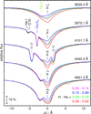 |
Fig. 5 Sections of the observed optical spectrum around H I Balmer lines and their respective He II blends compared with three synthetic spectra with Teff = 45 000 K and different H and He abundances (given in mass fraction, the labels’ colors refer to the respective spectra). A synthetic spectrum calculated with the photospheric parameters of Krtička et al. (2019) is shown in the line centers with a dashed, violet line. Prominent stellar and interstellar (subscript is) lines are marked. |
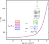 |
Fig. 6 Temperature structures of our models with log g = 4.46 and different Teff. The formation depths of the line cores of selected H I, He I, He II. C III, C IV, N III, and N IV lines (visible in our TUES or UVES observation) in our Teff = 47 000 K model are indicated. m is the column mass, measured from the outer boundary of our model atmospheres. |
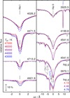 |
Fig. 7 Sections of the observed optical spectrum around prominent He I (left panel) and He II (right) lines compared to synthetic spectra with different Teff (the labels’ colors refer to the respective spectra). The two lower He II lines are compared with synthetic spectra with different log g. |
Wavelengths of the strongest metal lines used for the abundance determination.
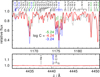 |
Fig. 8 Top panel: section of the TUES observation around С III λ λ 1174.93−1176.37Å and C IV λ λ 1168.89, 1168.98Å compared with our synthetic spectra with different C mass fractions (labeled with the logarithm, their colors indicate the respective synthetic spectra). Bottom: same as top panel, for a section of the UVES observation around He I λ 4437.55Å and C IV λ λ 4440.33−4441.73Å. |
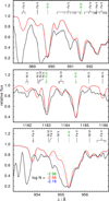 |
Fig. 9 Same as Fig. 8 but with the TUES observation and different N mass fractions around N III λ λ 989.80, 991.51, 991.58Å (top panel), N III λ λ 1182.97, 1183.03, 1184.51, 1184.57Å (middle), and N IV λ 954.47Å (bottom). |
5 Distance, luminosity, and mass
To determine the distance to a star, one can use the equivalent widths of the interstellar H and K lines (Са II λ λ 3968, 47, 3933.66Å). We measured  . These widths can then be used to calculate the distance by using formulae proposed by Megier et al. (2008),
 (1)
(1)
 (2)
(2)
The average d = 607 ± 80 pc is in agreement with the value previously determined by Kudritzki & Simon (1978, 650 ± 100), Krtička et al. (2019,508 ± 17), and  pc, which is calculated from parallax measurements5 by the Gaia mission.
Alternatively, the distance was calculated utilizing the Eddington flux at λ 5454 Åfollowing the formula6
 (3)
(3)
where M is the stellar mass in solar units,  /s/Hz the Eddington flux of our final model (Teff = 45 000 K, log g = 4.46, cf., Table 3) at λ 5454Å, and mv0 = mV−2.175 × c the extinction corrected apparent magnitude. Using EB−V = 0.038 ± 0.010, (Sect. 2, Fig. 3) and c = 1.47 EB−V from the standard stellar extinction curve (e.g., Osterbrock 1974), we calculate mv0 = 8.17 ± 0.03. This yields a distance of
  pc, in good agreement with previously determined values (Table 3), and a height below the Galactic plane of H = 163 ± 27 pc.
Using the Gaia distance and mV = 8.287 ± 0.0024 (Landolt & Uomoto 2007), the absolute magnitude is  . Using the bolometric-correction formula of Martins et al. (2005), we get
  , the luminosity can be approximated using the following formula taken from Martins et al. (2005),
 (4)
(4)
where  is the solar bolometric luminosity (Torres et al. 2010) and L☉ = 3.828 × 1033 erg/s is the solar luminosity (Mamajek et al. 2015).
The radius of HD 49798 is derived using the StefanBoltzmann law
 (5)
(5)
This radius is only slightly larger than the value by Krtička et al. (2019,1.05 ± 0.06 R☉), and is in agreement with the value calculated by Kudritzki & Simon (1978, 1.45 ± 0.25 R☉). Finally, the mass of HD 49798 is calculated using
 (6)
(6)
This mass is lower than the previously determined values of Krtička et al. (2019, 1.46 ± 0.32 M☉) and Kudritzki & Simon (1978, 1.75 ± 1.00 M☉) but agrees within the error limits.
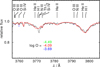 |
Fig. 11 Same as Fig. 10 but for different O mass fractions around О III λ λ 3757.23, 3759.88, 3791.28 Å. |
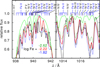 |
Fig. 12 Sections of the TUES observation compared with our synthetic spectra with different Fe abundances around some prominent Fe lines. |
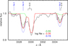 |
Fig. 14 Same as Fig. 12 but with different Ne abundances around Ne II λ λ 3327.153, 3334, 837Å and Ne III λ 3328.697Å. |
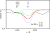 |
Fig. 15 Same as Fig. 11 but with different Mg abundances around Mg II λ λ 4481.12, 4481.14, 4481.32 Å. |
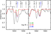 |
Fig. 16 Sections of the GHRS observations compared with our synthetic spectra with different Al abundances around Al III λ λ 1854.72, 1862.79Å. |
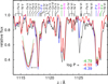 |
Fig. 17 Same as Fig. 8 but with different P abundances around P V λ λ 1117.98, 1128.01 Å (marked in blue). The thin, blue model spectrum includes interstellar line absorption. |
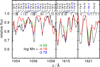 |
Fig. 18 Sections of the TUES panel) and GHRS (middle and right) observations compared with our synthetic spectra with different Mn abundances around Mn V λ λ 1055.06, 1055.98Å (left), Mn III λ 1614.96Å (middle), and Mn V λ 1621.03Å (right). |
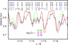 |
Fig. 19 Same as Fig. 17 but with different Cr mass fractions around Cr V λ λ 1112.45, 1114.35, 1116.48Å. We show the derived Cr abundance ± 0.4 dex for clarity. |
Determined stellar parameters, compared to previously determined values by Gaia, Krtička et al. (2019, K) and Kudritzki & Simon (1978, KS).
6 Results and conclusions
We performed a detailed spectral analysis of HD 49798 by means of advanced NLTE model-atmosphere techniques based on the available ORFEUS (TUES), HST/GHRS, and UVES spectra (Table 1). We found Teff = 45 000 ± 1000 K and log g = 4.46 ± 0.10, which is within the error limits (Table 4) and in good agreement with the results of Krtička et al. (2019) (Table 4). Our H/He mass-fraction ratio of 0.20/0.78 (Fig.5) agrees only marginally with the ratio of 0.25/0.74 (Table 4) that was found by Krtička et al. (2019).
We determined the photospheric abundances of H, He, C, N, O, Me, Al, Si, P, S, Cr, Mn, Fe, and Ni (Table 4, Fig. 20). A comparison of the ORFEUS, HST/GHRS, and UVES observations with our final TMAP spectrum is shown in Figs. A.1–A.3.
HD 49798 remains interesting regarding its origin and future evolution as it seems to deviate from most observations made regarding hot subdwarfs. Its low surface gravity of log g = 4.46 in combination with the high Teff = 45 000 K places it outside the known region in the log Teff−log g plane inhabited by sdOs (Fig. 21). Thus, HD 49798 did not pass the classical horizontalbranch (HB) or extended horizontal-branch (EHB) evolutionary scenario.
HD 49798 is a stripped, intermediate-mass He star. Brooks et al. (2017) calculated three MESA7 sdO models (Paxton et al. 2011, 2013, 2015) for a ZAMS star with MZAMS = 7.15 M☉ and different mass-loss rates to match Teff = 47 500 ± 2000 K and log g = 4.25 ± 0.2 of Kudritzki & Simon (1978). Their evolutionary tracks (digitized with Dexter8) are shown in Fig. 21. Our values of Teff = 45 000 ± 1000 K and log g = 4.46 ± 0.1 show HD 49798 just below these tracks, i.e., at a He-core mass of ≲ 1.4 M☉.
The CNO abundances of HD 49798 are in line with yields of the CNO cycle and 3 α nucleosynthesis. Significantly oversolar abundances of heavy elements like Cr, Mn, Fe, and Ni may be the result of diffusion. For HD 49798, Krtička et al. (2019) measured a mass-loss rate of Ṁ = 2.1 × 10⁻⁹ M☉/yr, which is too high for an efficient diffusion. This mass-loss rate is slightly lower than the value for an assumed solar composition 2.7 × 10⁻⁹ M☉/yr (cf., Krtička et al. 2019) and, thus, subsolar heavy-metal abundances would be expected.
However, we searched for lines of trans-iron elements (cf., Hoyer et al. 2017, 2018; Löbling et al. 2020; Rauch et al. 2020), but this was entirely unsuccessful. This was expected at the high v∞ = 1570 km/s (Krtička et al. 2019) and a height of the photosphere of ≈ 5 × 10⁴ km.
The compact companion of HD 49798 has a rotational period of 13.2 s (Israel et al. 1997) and a very high spinup rate. Mereghetti et al. (2021) analyzed results of XMM-Newton9 pointings and found a constant spin-up rate of Ṗ = (−2.17 ± 0.01) × 10−15 ss−1, which led them to presume it was a WD covered with helium-rich material accreted from HD 49798. Recently, Rigoselli et al. (2023) measured Ṗ = (−2.28 ± 0.02) × 10−15 ss−1 from NICER10, XMM-Newton, and ROSAT11 observations (together over a period of ≈ 30 years). Such a high spin-up cannot be explained by accretion alone due to the low mass transfer in this binary (Mereghetti et al. 2016). The scenario proposed by Popov et al. (2018) is more likely, in which the WD, which is only a few million years old, is contracting. An ongoing analysis of photometric TESS12 data (Schaffenroth et al., in prep.) will further improve the orbital parameters and our understanding of HD 49798.
We discovered a very good spectrum of HD 49798 (Fig. A.1) in the ORFEUS database (https://archive.stsci.edu/ tues/search.php) – observed but never analyzed or published. Without this observation, Krtička et al. (2019) could not evaluate C III λ λ 1174.93−1176.37Å and C IV λ λ 1168.89, 1168.98Å and derived only an upper C-abundance limit from the UVES observation. Their upper limit, however, is close to the value that we determined (Fig. 20). At least the prominent N IV and S VI P Cygni profiles (Fig. A.1) deserve further analysis; this is not possible with our hydrostatic TMAP. However, we expect there to be many other “forgotten” spectra in other archives, ready to be analyzed.
Parameters of HD 49798.
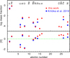 |
Fig. 20 Comparison of photospheric abundances of HD 49798 with the results of Krtička et al. (2019). The uncertainties of the abundances are given in Table 4. Arrows indicate upper limits. Top: abundances given as logarithmic mass fraction. Bottom: abundance ratios to the respective solar values (Asplund et al. 2009; Scott et al. 2015b,a). [X] denotes the log (mass fraction/solar mass fraction) of species X. The dashed green line indicates solar abundances. |
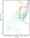 |
Fig. 21 Location of HD 49798 (red error ellipse) in the log Teff−log g plane compared with three MESA models for the evolution of He cores with different masses (orange tracks, evolution towards lower log g, taken from Brooks et al. 2017). The blue error ellipse shows the error limits of Krtička et al. (2019). Positions of sdB (Geier et al. 2017, blue, open squares), sdO stars (Geier 2020, green, open rhombs), and Hrich WDs (Gianninas et al. 2010, green, dashed lines) are indicated. Four post-EHB evolutionary tracks, labeled with the stellar mass in M☉, (Dorman et al. 1993, blue, dashed lines for Y = 0.459 ≈ 1.6 × Y☉) are shown to indicate their evolution. The dashed green lines indicate the He main sequence and the zero- and terminal-age EHB. |
Acknowledgements
We thank Klaus Werner for helpful comments, discussions, and for careful reading of the manuscript; Jiri Krtička for putting the reduced optical UVES spectrum, that had been used in Krtička et al. (2019), at our disposal; and Klaas de Boer, for many long-time-ago discussions about UV spectroscopy (especially about ORFEUS). This research has made use of the SIMBAD database, operated at CDS, Strasbourg, France, and of NASA’s Astrophysics Data System. The TIRO (http://astro.uni-tuebingen.de/~TIRO) tool and the TMAD (http://astro.uni-tuebingen.de/~TMAD) service were constructed as part of the Tübingen project (https://uni-tuebingen. de/de/122430) of the German Astrophysical Virtual Observatory (GAVO, http://www.g-vo.org). This work used the profile-fitting procedure OWENS developed by M. Lemoine and the FUSE French Team.
Appendix A Additional figures
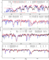 |
Fig. A.1 ORFEUS II observation (black) compared with our best model with (blue) and without (red) interstellar line absorption considered. vrad = 140 km/s and vrot = 37.5 km/s are applied to our model. Stellar lines are identified at top. Prominent PCyg profiles of N IV λ λ 922.0, 922.5, 923.1, 924.3Å, N V λ λ 1238.8, 1242.8 Å, and S VI λ λ 933.4, 944.5Å are indicated by horizontal bars. The green marks at the bottom of each panel indicate wavelengths and strengths (mark lengths ∼ log g f value of the respective line) of prominent iron-group (Ca−Ni) lines. |
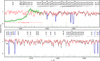 |
Fig. A.2 Like Fig. A.1 but for the GHRS observations. In the range of the N V λ λ 1238.8, 1242.8 Å P Cygni profile, the ORFEUS II spectrum (green) is shown for comparison. |
References
- Asplund, M., Grevesse, N., Sauval, A. J., & Scott, P., 2009, ARA&A, 47, 481 [NASA ADS] [CrossRef] [Google Scholar]
- Barnard, A. J., Cooper, J., & Smith, E. W., 1974, J. Quant. Spec. Radiat. Transf., 14, 1025 [Google Scholar]
- Barnard, A. J., Cooper, J., & Smith, E. W., 1975, J. Quant. Spec. Radiat. Transf., 15, 429 [Google Scholar]
- Branch, D., & Wheeler, J., 2017, Supernova Explosions, Astronomy and Astrophysics Library (Springer Berlin Heidelberg) [Google Scholar]
- Brooks, J., Kupfer, T., & Bildsten, L., 2017, ApJ, 847, 78 [NASA ADS] [CrossRef] [Google Scholar]
- Cannon, A. J., & Pickering, E. C., 1918, Ann. Harvard College Observ., 92, 1 [Google Scholar]
- Cutri, R. M., Skrutskie, M. F., van Dyk, S., et al. 2003, VizieR Online Data Catalog: II/246 [Google Scholar]
- Dimitrijević, M. S., & Sahal-Bréchot, S. 1992a, A&AS, 95, 109 [Google Scholar]
- Dimitrijević, M. S., & Sahal-Bréchot, S. 1992b, A&AS, 96, 613 [Google Scholar]
- Dimitrijevic, M. S., & Sahal-Brechot, S., 1995, A&AS, 109, 551 [Google Scholar]
- Dimitrijević, M. S., Sahal-Bréchot, S., & Bommier, V., 1991, A&AS, 89, 581 [Google Scholar]
- Dorman, B., Rood, R. T., & O’Connell, R. W., 1993, ApJ, 419, 596 [NASA ADS] [CrossRef] [Google Scholar]
- Dufton, P. L., 1972, MNRAS, 159, 79 [Google Scholar]
- Feast, M. W., Thackeray, A. D., & Wesselink, A. J., 1957, MmRAS, 68, 1 [NASA ADS] [Google Scholar]
- Fitzpatrick, E. L., 1999, PASP, 111, 63 [Google Scholar]
- Geier, S., 2020, A&A, 635, A193 [NASA ADS] [CrossRef] [EDP Sciences] [Google Scholar]
- Geier, S., Østensen, R. H., Nemeth, P., et al. 2017, A&A, 600, A50 [NASA ADS] [CrossRef] [EDP Sciences] [Google Scholar]
- Gianninas, A., Bergeron, P., Dupuis, J., & Ruiz, M. T., 2010, ApJ, 720, 581 [NASA ADS] [CrossRef] [Google Scholar]
- Griem, H. R., 1974, Spectral line Broadening by Plasmas (New York: Academic Press) [Google Scholar]
- Groenewegen, M. A. T., & Lamers, H. J. G. L. M., 1989, A&AS, 79, 359 [Google Scholar]
- Hamann, W. R., Gruschinske, J., Kudritzki, R. P., & Simon, K. P., 1981, A&A, 104, 249 [NASA ADS] [Google Scholar]
- Heber, U., 2016, PASP, 128, 08/2001 [Google Scholar]
- Hébrard, G., & Moos, H. W., 2003, ApJ, 599, 297 [Google Scholar]
- Hébrard, G., Friedman, S. D., Kruk, J. W., et al. 2002, Planet. Space Sci., 50, 1169 [CrossRef] [Google Scholar]
- Hoyer, D., Rauch, T., Werner, K., & Kruk, J. W., 2018, A&A, 612, A62 [NASA ADS] [CrossRef] [EDP Sciences] [Google Scholar]
- Hoyer, D., Rauch, T., Werner, K., Kruk, J. W., & Quinet, P., 2017, A&A, 598, A135 [NASA ADS] [CrossRef] [EDP Sciences] [Google Scholar]
- Hubeny, I., Hummer, D. G., & Lanz, T., 1994, A&A, 282, 151 [NASA ADS] [Google Scholar]
- Hummer, D. G., & Mihalas, D., 1988, ApJ, 331, 794 [NASA ADS] [CrossRef] [Google Scholar]
- Israel, G. L., Stella, L., Angelini, L., et al. 1997, ApJ, 474, L53 [NASA ADS] [CrossRef] [Google Scholar]
- Jaschek, M., & Jaschek, C., 1963, PASP, 75, 365 [NASA ADS] [CrossRef] [Google Scholar]
- Jeffery, C. S., Drilling, J. S., Harrison, P. M., Heber, U., & Moehler, S., 1997, A&AS, 125, 501 [NASA ADS] [CrossRef] [EDP Sciences] [Google Scholar]
- Krtička, J., Janík, J., Krtičková, I., et al. 2019, A&A, 631, A75 [NASA ADS] [CrossRef] [EDP Sciences] [Google Scholar]
- Kudritzki, R. P., 1976, A&A, 52, 11 [NASA ADS] [Google Scholar]
- Kudritzki, R. P., & Simon, K. P., 1978, A&A, 70, 653 [NASA ADS] [Google Scholar]
- Landolt, A. U., & Uomoto, A. K., 2007, AJ, 133, 768 [Google Scholar]
- Löbling, L., Maney, M. A., Rauch, T., et al. 2020, MNRAS, 492, 528 [Google Scholar]
- Mamajek, E. E., Torres, G., Prsa, A., et al. 2015, arXiv e-prints [arXiv:1510.06262] [Google Scholar]
- Martins, F., Schaerer, D., & Hillier, D. J., 2005, A&A, 436, 1049 [NASA ADS] [CrossRef] [EDP Sciences] [Google Scholar]
- Megier, A., Strobel, A., Bondar, A., et al. 2008, ApJ, 634, 451 [Google Scholar]
- Mereghetti, S., Tiengo, A., Esposito, P., et al. 2009, Science, 325, 1222 [NASA ADS] [CrossRef] [Google Scholar]
- Mereghetti, S., La Palombara, N., Tiengo, A., et al. 2011, ApJ, 737, 51 [NASA ADS] [CrossRef] [Google Scholar]
- Mereghetti, S., La Palombara, N., Tiengo, A., et al. 2013, A&A, 553, A46 [NASA ADS] [CrossRef] [EDP Sciences] [Google Scholar]
- Mereghetti, S., Pintore, F., Esposito, P., et al. 2016, MNRAS, 458, 3523 [NASA ADS] [CrossRef] [Google Scholar]
- Mereghetti, S., Pintore, F., Rauch, T., et al. 2021, MNRAS, 504, 920 [NASA ADS] [CrossRef] [Google Scholar]
- Müller-Ringat, E., 2013, Dissertation, University of Tübingen, Germany, http://nbn-resolving.de/urn:nbn:de:bsz:21-opus-67747 [Google Scholar]
- Napiwotzki, R., & Rauch, T., 1994, A&A, 285, 603 [NASA ADS] [Google Scholar]
- Nomoto, K., 1987, ApJ, 322, 206 [NASA ADS] [CrossRef] [Google Scholar]
- Oosterhoff, P. T., 1951, Bull. Astron. Inst. Netherlands, 11, 299 [Google Scholar]
- Osterbrock, D. E., 1974, Astrophysics of Gaseous Nebulae (San Francisco: W.H. Freeman Co.) [Google Scholar]
- Paxton, B., Bildsten, L., Dotter, A., et al. 2011, ApJS, 192, 3 [Google Scholar]
- Paxton, B., Cantiello, M., Arras, P., et al. 2013, ApJS, 208, 4 [Google Scholar]
- Paxton, B., Marchant, P., Schwab, J., et al. 2015, ApJS, 220, 15 [Google Scholar]
- Popov, S. B., Mereghetti, S., Blinnikov, S. I., Kuranov, A. G., & Yungelson, L. R., 2018, MNRAS, 474, 2750 [NASA ADS] [Google Scholar]
- Rauch, T., & Deetjen, J. L., 2003, in Astronomical Society of the Pacific Conference Series, 288, Stellar Atmosphere Modeling, eds. I. Hubeny, D. Mihalas, & K. Werner, 103 [Google Scholar]
- Rauch, T., Gamrath, S., Quinet, P., et al. 2020, A&A, 637, A4 [EDP Sciences] [Google Scholar]
- Richter, D., 1971, A&A, 14, 415 [Google Scholar]
- Rigoselli, M., De Grandis, D., Mereghetti, S., & Malacaria, C., 2023, MNRAS, 523, 3043 [Google Scholar]
- Savitzky, A., & Golay, M. J. E., 1964, Analyt. Chem., 36, 1627 [NASA ADS] [CrossRef] [Google Scholar]
- Schöning, T., & Butler, K., 1989, A&AS, 78, 51 [Google Scholar]
- Scott, P., Asplund, M., Grevesse, N., Bergemann, M., & Sauval, A. J. 2015a, A&A, 573, A26 [NASA ADS] [CrossRef] [EDP Sciences] [Google Scholar]
- Scott, P., Grevesse, N., Asplund, M., et al. 2015b, A&A, 573, A25 [NASA ADS] [CrossRef] [EDP Sciences] [Google Scholar]
- Thackeray, A. D., 1970, MNRAS, 150, 215 [NASA ADS] [CrossRef] [Google Scholar]
- Torres, G., Andersen, J., & Giménez, A., 2010, A&A Rev., 18, 67 [Google Scholar]
- Tremblay, P.-E., & Bergeron, P., 2009, ApJ, 696, 1755 [Google Scholar]
- Werner, K., Dreizler, S., & Rauch, T., 2012, TMAP: Tübingen NLTE Model-Atmosphere Package, Astrophysics Source Code Library [record ascl:1212.015] [Google Scholar]
Modules for Experiments in Stellar Astrophysics, Paxton et al. (2011, 2013, 2015).
Orbiting and Retrievable Far- and Extreme Ultraviolet Spectrometer.
Gaia source_id: 5562023884304074240.
Modules for Experiments in Stellar Astrophysics.
X-ray Multi Mirror Mission.
Neutron Star Interior Composition Explorer.
Röntgen Satellit.
Telescope Encoder and Sky Sensor.
All Tables
Determined stellar parameters, compared to previously determined values by Gaia, Krtička et al. (2019, K) and Kudritzki & Simon (1978, KS).
All Figures
|
Fig. 1 Classification scheme for hot subdwarf stars by Jeffery et al. (1997). The red box denotes the classification of HD 49798. |
| In the text | |
|
Fig. 2 Section of the TUES observation around Ly α (black). The interstellar H I absorption was calculated with NH I = 1.8 (full, red) ± 0.5 (dashed, red, 2.5 times the estimated error range for clarity) × 1020 cm−2. The pure stellar spectrum is shown in blue. A rotational line broadening (vrot = 37.5 km/s) is applied. Interstellar metal lines are not modeled in this plot. The P Cygni profile of the N V resonance line is marked at the top. |
| In the text | |
|
Fig. 3 TUES, GHRS, and IUE observations compared with our final model normalized to the 2MASS H magnitude. EB−v = 0.038 ± 0.010 is applied. In addition, the B and V magnitudes (Landolt & Uomoto 2007) as well as the 2MASS J, H, and Ks magnitudes (Cutri et al. 2003) are shown. For clarity, TUES and GHRS spectra are convolved with a Gaussian with a full width at half maximum (FWHM) of 7Å. |
| In the text | |
|
Fig. 4 Our final model spectrum with different vrot(30−50 km/s, the labels’ colors refer to the respective spectra) applied, compared with a section of the UVES observation around N III λ λ 3998.63, 4003.58Å. |
| In the text | |
|
Fig. 5 Sections of the observed optical spectrum around H I Balmer lines and their respective He II blends compared with three synthetic spectra with Teff = 45 000 K and different H and He abundances (given in mass fraction, the labels’ colors refer to the respective spectra). A synthetic spectrum calculated with the photospheric parameters of Krtička et al. (2019) is shown in the line centers with a dashed, violet line. Prominent stellar and interstellar (subscript is) lines are marked. |
| In the text | |
|
Fig. 6 Temperature structures of our models with log g = 4.46 and different Teff. The formation depths of the line cores of selected H I, He I, He II. C III, C IV, N III, and N IV lines (visible in our TUES or UVES observation) in our Teff = 47 000 K model are indicated. m is the column mass, measured from the outer boundary of our model atmospheres. |
| In the text | |
|
Fig. 7 Sections of the observed optical spectrum around prominent He I (left panel) and He II (right) lines compared to synthetic spectra with different Teff (the labels’ colors refer to the respective spectra). The two lower He II lines are compared with synthetic spectra with different log g. |
| In the text | |
|
Fig. 8 Top panel: section of the TUES observation around С III λ λ 1174.93−1176.37Å and C IV λ λ 1168.89, 1168.98Å compared with our synthetic spectra with different C mass fractions (labeled with the logarithm, their colors indicate the respective synthetic spectra). Bottom: same as top panel, for a section of the UVES observation around He I λ 4437.55Å and C IV λ λ 4440.33−4441.73Å. |
| In the text | |
|
Fig. 9 Same as Fig. 8 but with the TUES observation and different N mass fractions around N III λ λ 989.80, 991.51, 991.58Å (top panel), N III λ λ 1182.97, 1183.03, 1184.51, 1184.57Å (middle), and N IV λ 954.47Å (bottom). |
| In the text | |
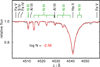 |
Fig. 10 Same as Fig. 9 but showing the UVES observation around N III λ λ 4510−4547Å. |
| In the text | |
|
Fig. 11 Same as Fig. 10 but for different O mass fractions around О III λ λ 3757.23, 3759.88, 3791.28 Å. |
| In the text | |
|
Fig. 12 Sections of the TUES observation compared with our synthetic spectra with different Fe abundances around some prominent Fe lines. |
| In the text | |
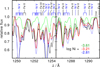 |
Fig. 13 Same as Fig. 12 but with different Ni abundances around some prominent Ni lines. |
| In the text | |
|
Fig. 14 Same as Fig. 12 but with different Ne abundances around Ne II λ λ 3327.153, 3334, 837Å and Ne III λ 3328.697Å. |
| In the text | |
|
Fig. 15 Same as Fig. 11 but with different Mg abundances around Mg II λ λ 4481.12, 4481.14, 4481.32 Å. |
| In the text | |
|
Fig. 16 Sections of the GHRS observations compared with our synthetic spectra with different Al abundances around Al III λ λ 1854.72, 1862.79Å. |
| In the text | |
|
Fig. 17 Same as Fig. 8 but with different P abundances around P V λ λ 1117.98, 1128.01 Å (marked in blue). The thin, blue model spectrum includes interstellar line absorption. |
| In the text | |
|
Fig. 18 Sections of the TUES panel) and GHRS (middle and right) observations compared with our synthetic spectra with different Mn abundances around Mn V λ λ 1055.06, 1055.98Å (left), Mn III λ 1614.96Å (middle), and Mn V λ 1621.03Å (right). |
| In the text | |
|
Fig. 19 Same as Fig. 17 but with different Cr mass fractions around Cr V λ λ 1112.45, 1114.35, 1116.48Å. We show the derived Cr abundance ± 0.4 dex for clarity. |
| In the text | |
|
Fig. 20 Comparison of photospheric abundances of HD 49798 with the results of Krtička et al. (2019). The uncertainties of the abundances are given in Table 4. Arrows indicate upper limits. Top: abundances given as logarithmic mass fraction. Bottom: abundance ratios to the respective solar values (Asplund et al. 2009; Scott et al. 2015b,a). [X] denotes the log (mass fraction/solar mass fraction) of species X. The dashed green line indicates solar abundances. |
| In the text | |
|
Fig. 21 Location of HD 49798 (red error ellipse) in the log Teff−log g plane compared with three MESA models for the evolution of He cores with different masses (orange tracks, evolution towards lower log g, taken from Brooks et al. 2017). The blue error ellipse shows the error limits of Krtička et al. (2019). Positions of sdB (Geier et al. 2017, blue, open squares), sdO stars (Geier 2020, green, open rhombs), and Hrich WDs (Gianninas et al. 2010, green, dashed lines) are indicated. Four post-EHB evolutionary tracks, labeled with the stellar mass in M☉, (Dorman et al. 1993, blue, dashed lines for Y = 0.459 ≈ 1.6 × Y☉) are shown to indicate their evolution. The dashed green lines indicate the He main sequence and the zero- and terminal-age EHB. |
| In the text | |
|
Fig. A.1 ORFEUS II observation (black) compared with our best model with (blue) and without (red) interstellar line absorption considered. vrad = 140 km/s and vrot = 37.5 km/s are applied to our model. Stellar lines are identified at top. Prominent PCyg profiles of N IV λ λ 922.0, 922.5, 923.1, 924.3Å, N V λ λ 1238.8, 1242.8 Å, and S VI λ λ 933.4, 944.5Å are indicated by horizontal bars. The green marks at the bottom of each panel indicate wavelengths and strengths (mark lengths ∼ log g f value of the respective line) of prominent iron-group (Ca−Ni) lines. |
| In the text | |
|
Fig. A.2 Like Fig. A.1 but for the GHRS observations. In the range of the N V λ λ 1238.8, 1242.8 Å P Cygni profile, the ORFEUS II spectrum (green) is shown for comparison. |
| In the text | |
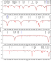 |
Fig. A.3 Like Fig. A.1 but for the UVES observation. |
| In the text | |
Current usage metrics show cumulative count of Article Views (full-text article views including HTML views, PDF and ePub downloads, according to the available data) and Abstracts Views on Vision4Press platform.
Data correspond to usage on the plateform after 2015. The current usage metrics is available 48-96 hours after online publication and is updated daily on week days.
Initial download of the metrics may take a while.