| Issue |
A&A
Volume 700, August 2025
|
|
|---|---|---|
| Article Number | A149 | |
| Number of page(s) | 10 | |
| Section | Extragalactic astronomy | |
| DOI | https://doi.org/10.1051/0004-6361/202555345 | |
| Published online | 13 August 2025 | |
Toward an observational detection of halo spin bias using spin-orbit coherence
1
Astronomy Program, Department of Physics and Astronomy, Seoul National University, 1 Gwanak-ro, Gwanak-gu, Seoul 08826, Republic of Korea
2
Departamento de Física, Universidad Técnica Federico Santa María, Avenida Vicuña Mackenna 3939, San Joaquín, Santiago, Chile
3
Departamento de Física, Universidad Técnica Federico Santa María, Avenida España 1680, Valparaíso, Chile
4
Millenium Nucleus for Galaxies (MINGAL), Santiago, Chile
5
Korea Astronomy and Space Science Institute (KASI), 776 Daedeokdae-ro, Yuseong-gu, Daejeon 34055, Republic of Korea
⋆ Corresponding authors: This email address is being protected from spambots. You need JavaScript enabled to view it.
, This email address is being protected from spambots. You need JavaScript enabled to view it.
, This email address is being protected from spambots. You need JavaScript enabled to view it.
Received:
30
April
2025
Accepted:
23
June
2025
Abstract
Context. The clustering of dark-matter halos depends primarily on halo mass. However, when using a fixed halo mass, numerical simulations have been able to reveal multiple secondary dependencies. This so-called secondary halo bias has important implications for our understanding of structure formation and observational cosmology. Despite its significance, the effect has not yet been measured observationally with statistical confidence.
Aims. We aim to develop the first observational method to probe halo spin bias: the secondary dependence of halo clustering on halo spin at a fixed halo mass.
Methods. We used a proxy for halo spin based on the coherent motion of galaxies within and around a halo. We tested this technique using the IllustrisTNG hydrodynamical simulation and subsequently applied it to a group catalog from the Sloan Digital Sky Survey (SDSS). By splitting the SDSS groups according to this spin proxy and measuring the two-point correlation function of the resulting samples, we investigated the existence of halo spin bias.
Results. We find consistent indications that at a fixed mass, groups with higher values for the spin proxy exhibit a higher bias than those with lower spin proxy values on scales of 5−15 h−1 Mpc. The highest significance was observed for groups with halo masses Mh ≳ 1013.2h−1 M⊙, for which 85% of the sampled measurements display the expected trend. As we continue to improve on the method, our results could open new avenues for studying the connection between halo spin and the large-scale structure through the use of upcoming spectroscopic surveys.
Key words: galaxies: evolution / galaxies: kinematics and dynamics / large-scale structure of Universe
© The Authors 2025
 Open Access article, published by EDP Sciences, under the terms of the Creative Commons Attribution License (https://creativecommons.org/licenses/by/4.0), which permits unrestricted use, distribution, and reproduction in any medium, provided the original work is properly cited.
This article is published in open access under the Subscribe to Open model. This email address is being protected from spambots. You need JavaScript enabled to view it. to support open access publication.
1. Introduction
In the so-called non-linear regime of structure formation, overdensities of dark matter (DM) can decouple from the expansion of the Universe and continue collapsing to form DM halos. Within these collapsed objects, which constitute the building blocks of the large-scale structure (LSS) of the Universe, galaxies form by cooling and condensation of gas inside the halos’ potential wells (White & Rees 1978; White & Frenk 1991). In this context, linear halo bias describes the relation between the density contrast of DM halos and that of the underlying matter density field on large scales, i.e, bh = δh/δm (e.g., Mo & White 1996). It can be easily shown that this parameter also indicates the relative clustering strength of both components, as bh2 = ξh/ξm, where ξh and ξm are the auto-correlation functions of halos and matter.
It is well known that halo bias depends strongly on the internal properties of halos. Halo mass is responsible for the primary dependence, which is a direct manifestation of the more fundamental dependence of halo bias on the peak height of density fluctuations, ν. As described by the Lambda cold dark matter (Λ-CDM) structure formation formalism, more massive halos are more tightly clustered than less massive halos (e.g., Press & Schechter 1974; Sheth & Tormen 1999, 2002; Sheth et al. 2001). At a fixed halo mass, a number of additional secondary dependencies have been unveiled using mostly cosmological simulations (see, e.g., Sheth & Tormen 2004; Gao et al. 2005; Wechsler et al. 2006; Gao & White 2007; Angulo et al. 2008; Li et al. 2008; Faltenbacher & White 2010; Lazeyras et al. 2017; Salcedo et al. 2018; Han et al. 2019; Mao et al. 2018; Sato-Polito et al. 2019; Johnson et al. 2019; Ramakrishnan et al. 2019; Montero-Dorta et al. 2020, 2021a, 2025; Tucci et al. 2021; Montero-Dorta & Rodriguez 2024). As an example, lower mass halos that assemble a significant portion of their mass early on are more tightly clustered than those that form at later times, an effect referred to as “halo assembly bias”.
Another secondary halo bias effect that has been discussed in the literature is the so-called spin bias, the dependence on halo spin, λ (e.g., Gao & White 2007; Sato-Polito et al. 2019; Johnson et al. 2019; Tucci et al. 2021; Montero-Dorta et al. 2021b; Montero-Dorta 2021). Halo spin is commonly defined in simulations as a dimensionless parameter proportional to the total angular momentum of the DM particles (Peebles 1969; Bullock et al. 2001), namely:
 (1)
(1)
for the Bullock et al. version, where J is the halo angular momentum inside a sphere of radius, Rvir, and mass, Mvir, and Vvir is its circular velocity at virial radius, Rvir. The effect of spin bias on the clustering of halos can be divided into two regimes. At the low-mass end, lower-spin halos are more tightly clustered than higher-spin halos of the same mass due to the effect of splashback halos (Tucci et al. 2021). At the high-mass end, the opposite trend is observed. It appears that this “intrinsic” dependence could be related to fundamental theories that link the angular momentum of halos to the tidal field (e.g., such as the tidal torque theory Barnes & Efstathiou 1987). However, the physical origins of spin bias, and secondary bias in general, are yet to be established (see, e.g., Dalal et al. 2008; Paranjape et al. 2018; Montero-Dorta et al. 2025).
Although secondary halo bias has been extensively characterized from cosmological simulations, its existence is yet to be established observationally. The attempts to probe the effect can be divided in two groups. Some works have focused on demonstrating the halo bias effect directly from observations, using proxies for halo properties (e.g., Miyatake et al. 2016; Lin et al. 2016; Montero-Dorta et al. 2017; Niemiec et al. 2018; Sunayama et al. 2022). Other works have addressed the manifestation of secondary halo bias in the galaxy population, an effect that is generally called “galaxy assembly bias” (see, e.g., Obuljen et al. 2020; Salcedo et al. 2022; Wang et al. 2022 – we note that different definitions of this effect are assumed). Despite some claims, it is fair to say that a broadly accepted proof for the existence of secondary bias has not been presented due to a variety of issues, including selection and contamination effects, the small amplitude of the signal for assembly bias in some ranges, and the inherent challenge of measuring halo masses, to name but a few.
In this work, we investigate, for the first time, halo spin bias using observational data. At face value, spin bias provides a major advantage as compared to halo assembly bias in terms of a potential detection of secondary bias. Unlike assembly bias, the spin-bias signal increases in amplitude toward the high-mass end (e.g., Tucci et al. 2021), which allows for the use of clusters to probe the effect. Conversely, however, measuring the spin of halos has historically been very challenging (Mroczkowski et al. 2019). Montero-Dorta et al. (2021b) presented a proof of concept analysis on the feasibility of the rotational kinetic Sunyaev Zel’dovich (rkSZ) effect as the basis of a potential observational probe for halo spin bias. Although the correlation between the rkSZ signal and halo spin in hydrodynamical simulations is indeed sufficient to produce secondary bias, the observational aspects of the rkSZ measurement still represent a major obstacle (Mroczkowski et al. 2019).
Our observational probe for spin bias is based on the coherent orbital motion of neighboring galaxies around a target halo. This proxy has already been measured observationally in Lee et al. (2019a,b). In these works, the spin direction of the target galaxy is found to correlate with the averaged motion of galaxies around the target galaxy. Using simulations, Kim et al. (2022) evaluated the factors that determine the strength of this coherence signal, finding that it increases with the mass of the target halo and its spin, λ. Thus, by measuring the motions of neighboring galaxies about a target halo, an estimate for the magnitude and direction of its spin vector can be obtained. We refer to this coherence as the “spin-orbit coherence” (SOC). We also refer to the magnitude of the coherence motion as the “coherence signal” for simplicity. The observational probe presented here opens up the doorway for an observational analysis of halo spin bias, which could provide an important validation of the ΛCDM model.
The paper is structured as follows. In Sect. 2, we introduce the data employed in this work, including both the observational and simulation data. Sect. 3 describes the methodology that we follow, with special emphasis on our spin proxy based on SOC. In Sect. 4, we present the main result of the paper: our measurement of spin bias. Sect. 5 is devoted to discussing the robustness and significance of our measurement. Finally, in Sect. 6, we summarize our main conclusions and discuss the implications of our results. Throughout this work, we adopt the standard ΛCDM cosmology (Planck Collaboration XIII 2016), with parameters Ωm = 0.3089, Ωb = 0.0486, ΩΛ = 0.6911, H0 = 100 h km s−1 Mpc−1 with h = 0.6774, σ8 = 0.8159, and ns = 0.9667.
2. Data
Our analysis is based on publicly available data from both a hydrodynamical simulation, which we used to test the feasibility of our spin proxy, and a spectroscopic survey, where the spin-bias probe was applied. In this section, we describe the data and the selection criteria for both data sets.
2.1. Illustris TNG300
Part of our analysis is based on data from the Illustris-TNG magneto-hydrodynamical cosmological simulation (hereafter TNG for simplicity, Pillepich et al. 2018a,b; Nelson et al. 2018, 2019; Marinacci et al. 2018; Naiman et al. 2018; Springel et al. 2018). The TNG simulation suite was produced using the AREPO moving-mesh code (Springel 2010) and is considered an improved version of the previous Illustris simulation (Vogelsberger et al. 2014a,b; Genel et al. 2014). The updated TNG sub-grid models account for star formation; radiative metal cooling; chemical enrichment from SNII, SNIa, and AGB stars; and stellar and super-massive black hole feedback. These models were calibrated to successfully reproduce a set of observational constraints that include the observed z = 0 galaxy stellar mass function, the cosmic star formation rate (SFR) density, the halo gas fraction, the galaxy stellar size distributions, and the black hole–galaxy mass relation (we refer the reader to the aforementioned papers for more information).
We analyzed the largest box available in the database, TNG300-1 (hereafter TNG3001), which provides an obvious advantage when it comes to measuring large-scale halo and galaxy clustering. TNG300 spans a side length of 205 h−1 Mpc and includes periodic boundary conditions. The TNG300 run followed the dynamical evolution of 25003 DM particles of mass 4.0 × 10⁷ h−1 M⊙ and (initially) 25003 gas cells of mass 7.6 × 10⁶ h−1 M⊙.
To ensure mass resolution, we imposed mass cuts of Mh > 1011 h−1 M⊙ and Msh > 109 h−1 M⊙ for the total mass of bound particles in halos and subhalos, respectively2. These selection criteria reduced the sample to 254 382 halos and more than 107 subhalos.
Since our aim is to compare simulation and observational data directly, we created a mock catalog from TNG300. This mock catalog was constructed by converting the z = 0 TNG300 snapshot into a 2D projected catalog and placing the observer at the center of the box. It contains positions, masses, velocities, and the R200 radii for halos along with positions, masses, and velocities for subhalos (galaxies). These properties are required to measure the average motion of galaxies around each halo. We used this mock catalog as a reference to evaluate the impact of projection effects on the measurement of spin bias and to aid in the optimization of certain parameters of our spin proxy. However, we note that it is not fully comparable to the observational data from Sloan Digital Sky Survey (SDSS) in terms of neighbor mass distributions, owing to intrinsic differences between the TNG simulation and our SDSS galaxy and group selection criteria. The SDSS selection is discussed in the following section.
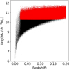 |
Fig. 1. Stellar mass (M*) versus redshift for galaxies in the SDSS LowZ catalog. Black markers show the entire sample, while the red markers show our volume-limited sample. |
2.2. The SDSS LowZ group catalog
The observational data employed in this work are part of the SDSS Data Release 13 (SDSS DR13; Albareti et al. 2017), which provides spectroscopy for galaxies throughout a large cosmological volume. These two aspects are crucial for our analysis, as the coherence measurement requires the precision of spectroscopic redshifts, while the clustering determination needs large cosmological volumes. The SDSS groups were extracted from the group catalog of Lim et al. (2017), hereafter referred to as the “SDSS LowZ group catalog”, which adopts a redshift limit of z < 0.2 and the r-band magnitude limit of the legacy survey (r < 17.77). Briefly, the group-finding algorithm from Lim et al. (2017) proceeds in an iterative way. First, the algorithm estimates the mass of the halo according to the stellar mass of its central galaxy following an abundance-matching approach. Then, the group’s size and velocity dispersion are evaluated in order to select the members. (For a complete description of the method, we refer the reader to Yang et al. 2005; Lim et al. 2017). Importantly, we used the halo mass-size relation from Pasquali et al. (2019) to determine the virial radius (R200) of each group:
![Mathematical equation: $$ \begin{aligned} R_{200}[\mathrm{h^{-1}\,kpc}] = \frac{258.1 * M_{\mathrm{h,*} }^{1/3} * (\Omega _{\rm m}/0.25)^{1/3}}{1+z}, \end{aligned} $$](/articles/aa/full_html/2025/08/aa55345-25/aa55345-25-eq2.gif) (2)
(2)
where Mh, * is the halo mass in units of 1012 h−1 M⊙ and Ωm is the total matter density in the Universe.
The secondary bias dependencies, including spin bias, are known to display significant redshift evolution, due to the intrinsic dependence on peak height (e.g., Gao & White 2007; Tucci et al. 2021). In order to minimize this effect and avoid issues related to incompleteness, we employed volume-limited samples, as shown in Fig. 1. In particular, we imposed a stellar mass cut of M* > 1010.3 h−1 M⊙, which ensures that the sample is complete in the redshift range 0.02 < z < 0.2; this is the sample we use throughout this work (red dots in Fig. 1). The stellar mass was estimated from the r-band luminosity and the g − r color following the prescription of Bell et al. (2003). This selection produced a sample of 410 042 galaxies.
Finally, it was important to impose a minimum number of group members in order to guarantee the robustness of our SOC measurements while ensuring high-number statistics for our group sample. This was achieved by considering only groups with at least three members. We checked that increasing this threshold to five members, for example, would result in significantly noisier results, and in that case, the number of groups decreased considerably. After imposing a cut of at least three members, the number of groups in our catalog totaled 22 456.
3. Method
3.1. Spin-orbit coherence
Our spin proxy based on the SOC is described in this section. The first evidence of this type of coherence was reported by Lee et al. (2019a) using the Calar Alto Legacy Integral Field spectroscopy Area (CALIFA) survey (Sánchez et al. 2012, 2016; Walcher et al. 2014). In that work, the spin of individual galaxies was measured using integrated field unit (IFU) data. Further work, presented in Lee et al. (2019b), showed the existence of a clear correlation between the spin direction of a central galaxy and the peculiar motion of the surrounding neighbor galaxies. The motion of the neighbor galaxies tends to align with the spin vector of their central galaxy. The parameter dependencies of this correlation in terms of the DM component were measured using cosmological simulations in Kim et al. (2022). In particular, Kim et al. (2022) revealed a strong relation between the halo spin parameter, λ, and the strength of the coherence of neighbor motions.
We measured the coherence signal by taking a mass weighted mean of the tangential velocities of neighboring galaxies, which we determined with respect to the central (host) halo3. These velocities were subsequently normalized by the virial velocity of the central halo since more massive halos tend to have higher neighbor velocities. By doing so, we were able to mitigate the intrinsic dependence of the coherence signal on the host halo mass. This is desirable because the halo spin parameter is, by construction, not strongly halo-mass dependent (Peebles 1969; Bullock et al. 2001).
An illustration of the procedure to measure the spin proxy is shown in Fig. 2. We only used galaxies that fall within the shaded X-shaped region to calculate the signal. The opening angle of the X-shaped region was set to 45°, following previous works (Lee et al. 2019a,b). The aim was to exclude galaxies that would not be expected to provide much signal, as they are close to the spin vector describing the rotation of the central halo. After the projected X cut was made about the halo, the mass weighted average of the line-of-sight velocity on either side of it was subsequently calculated. Galaxies on one side of the X region tend to move toward to the observer (negative velocities), while on the other side they move away from the observer (positive velocities), and this contributes to the strength of the spin proxy.
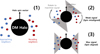 |
Fig. 2. Simplified illustration of the concept behind spin proxy based on SOC and its measurement. Illustration 1 depicts the SOC itself, while illustrations 2 and 3 show how the spin direction is determined by identifying the direction in which the coherence signal is strongest. |
Importantly, we set the region for identifying neighbor galaxies to 1 R200 on the sky and the velocity equivalent of 1 R200 along the line of sight, assuming a purely Hubble flow. This is a relatively narrow velocity cut that naturally excludes some cluster members. Our analysis using the TNG300 mock revealed that a narrow velocity cut produces a stronger signal, perhaps because we only consider the most relaxed members of the cluster in the calculation of the coherence signal. In addition, a narrow velocity cut helps mitigate the impact of external environmental effects from accidental inclusion of neighboring galaxies at greater distances. This potential contamination could artificially impact the signal. We come back to this point in Sect. 4.3, where we quantify the effect of varying the parameters of the fiducial model on the spin bias measurement.
Observationally, we do not know the spin direction of the galaxy groups and clusters. To try to determine its direction, we therefore first set an arbitrary direction for the halo spin vector and measured the coherence signal. Then, we smoothly turned it around by steps of 10° through 360° and calculated the coherence signal at each step. Our best choice for the direction of the spin vector is the step with the greatest value of coherence signal. The method to find the spin vector is shown in diagrams 2 and 3 of Fig. 2. We tested several choices of angle step size from 10 to 30°, and we found that this choice does not significantly affect our results.
Using TNG300 mock, we tested several conditions to maximize the correlation signal between λ and the SOC. We found that this correlation is most sensitive to the host halo’s mass, becoming significant for the range Mh > 1012 h−1 M⊙. On the other hand, we checked that the mass of the neighbors does not significantly affect the signal (see also Kim et al. 2022).
Finally, the correlation between the true spin and the spin proxy that motivates this analysis is shown in Fig. 3 using 3D measurements from TNG300. We note that there is a clear correlation above Mh = 1012 h−1 M⊙, which becomes stronger toward the high-mass end.
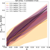 |
Fig. 3. Correlation between the spin proxy and the true halo spin (λ) for several host halo mass bins in TNG300. The solid lines show the mean of the distribution, while the shaded regions indicate the interquartile range (25th to 75th percentiles). These measurements have been performed in 3D. |
3.2. The spin bias measurement
We measured the halo spin bias, i.e., the secondary dependence of halo bias on spin at a fixed halo mass, both in simulations and observations by following the standard procedure for secondary bias based on the ratio of correlation functions (see, e.g., Salcedo et al. 2018; Sato-Polito et al. 2019; Montero-Dorta et al. 2020). In essence, we computed the correlation function for percentile subsets of halos based on their λ and spin proxy in bins of halo mass. As mentioned before, the main dependence of halo bias is known to be virial mass, as it is a direct manifestation of the more fundamental dependence on the peak height of density fluctuations (e.g., Sheth et al. 2001). Fig. 4 displays the auto-correlation function for groups as a function of mass in the SDSS LowZ group catalog, revealing the following well-known relation: more massive groups have a progressively higher clustering amplitude. This is an important sanity check for our analysis, and it gives us confidence that the secondary dependencies at a fixed halo mass can be measured observationally. We note that the mass binning adopted in Fig. 4 was also employed throughout our spin-bias measurement using SDSS LowZ group catalog. (Sect. 4.2).
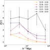 |
Fig. 4. Cross-correlation function of the SDSS LowZ group catalog as a function of group mass. The group mass range (log(Mh/h−1 M⊙)) of each measurement is indicated in the legend. As predicted from theory, more massive groups are more strongly clustered, which is the primary dependency of halo bias. |
The relative bias for a subset of halos based on λ (or, equally, the spin proxy) with respect to the entire halo population within a certain mass bin, i.e. bλ(r, Mh), can be computed as follows:
 (3)
(3)
where ξλ(r, Mh) is the cross-correlation between the corresponding λ or spin proxy percentile subset in that bin and the entire halo sample, and ξtot(r, Mh) is the cross-correlation between the whole mass bin and the entire halo sample (see Montero-Dorta et al. 2020 for more details). A difference between the relative bias of higher- and lower-spin (or spin proxy) subsets at a fixed halo mass would give rise to the secondary bias effect. Here, we used percentile subsets encompassing the upper and lower fractions of the mass bin (50−50% subsets). The cross-correlation functions were estimated by applying the traditional Landy & Szalay (1993) method. The calculation was done using the CORRFUNC code (Sinha & Garrison 2020), and the relative bias was averaged on scales of 5 − 15 h−1 Mpc (Montero-Dorta et al. 2020). For the randoms, we used ten times more objects than the data while also mimicking the geometry and volume of the data set (in the case of the SDSS, this includes mimicking the SDSS redshift distribution for the volume-limited sample).
An important aspect in the determination of secondary bias is the error computation, both in the SDSS LowZ group catalog and in TNG300 mock. Two different ways of estimating errors were employed in this work, depending on the secondary parameter used, for the sake of consistency. In TNG300, when λ, the real spin value, was used to split the halo population at fixed halo mass, errors were estimated using a traditional jackknife technique since statistics allow it. In this case, the TNG300 simulation box was divided into eight equal-volume sub-boxes, and eight different spin-bias measurements were obtained by excluding only one sub-box at a time. The errors correspond to the standard deviation of this set of measurements. In the SDSS LowZ group catalog, employing a jackknife error estimation was problematic due to low number statistics. For this reason, errors on the spin proxy measurements were determined using a bootstrap technique for each mass bin. A total of 100 bootstrap resampling subsets were generated. From these subsets, the mean and standard deviation of the resulting correlation functions were obtained. For consistency, this methodology was replicated in TNG300 whenever the spin proxy was employed, which helped us compare results between the observational data and thesimulation.
In order to ensure the robustness of our measurement, two additional checks were performed in the SDSS LowZ group catalog. First, we verified that the redshift distributions of the entire group sample, as well as the higher- and lower-spin subsets, are similar in each mass bin. Second, since the distribution of halo masses is not uniform across the mass range of interest, we set the binning so that each bin contains an equal number of halos. This scheme was adopted for all measurements. The set of parameters used for probing the spin bias in the SDSS group is summarized in Table 1.
Fiducial configuration for the spin bias measurement in the SDSS LowZ group catalog.
4. Results
In this section, we use our spin proxy to probe for spin bias observationally. We first report how we tested our method on the TNG300 mock in order to evaluate the feasibility of the measurement. Subsequently, we applied the method to the SDSS LowZ group catalog, and the robustness and significance of the resulting measurement were evaluated.
4.1. Testing the spin proxy in the simulation
To demonstrate that the spin proxy based on SOC is a reliable tracer of halo spin, we first tested it using simulations. As shown in Montero-Dorta et al. (2020), the TNG300 simulated halo population displays a significant halo spin bias, among other secondary dependencies of halo clustering. To evaluate the feasibility of our spin proxy, we first performed the halo spin bias measurement in the TNG300 mock catalog. These results are shown shown in Fig. 5. Each subset of halos corresponds to the 50% upper (orange) and lower (cyan) half of the λ distribution in each mass bin. The 1σ jackknife error of the relative bias is plotted as shaded regions, estimated using a set of sub-volumes, as described in Sect. 3.2. Despite the fact that we used projected quantities to match the observations, the spin bias signal still remains, i.e., for all mass bins, the orange lines are above the cyan lines. It is noteworthy that when measured from a sufficiently large simulation box, the signal for λ is known to continue to increase with halo mass (see, e.g., Sato-Polito et al. 2019), which is not clearly seen here at the highest masses due to low-number statistics.
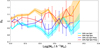 |
Fig. 5. Halo spin bias measured in projection from the TNG300 mock. Higher spin and higher spin proxy measurements are shown in orange and red solid lines and symbols, while the lower spin and lower spin proxy measurements are represented by cyan and blue solid lines, respectively. (See text for information regarding the computation of errors.) |
After we verified that the spin bias signal remains when the measurement is performed in projection, we repeated the analysis in the mock using the spin proxy instead of the λ parameter. These results are represented by the red and blue points in Fig. 5. Again, we used the 50% highest (red) and lowest (blue) spin-proxy values. We recall that when the spin proxy is used to estimate secondary bias, errors are calculated by bootstrapping. Fig. 5 demonstrates that the spin proxy shows a similar qualitative behavior in terms of spin bias as the λ-based measurement. This gives us confidence that the proxy can be successfully applied to observations, as we discuss in the following section.
4.2. Measuring spin bias in observations
Having confirmed that the spin proxy can be used to measure spin bias in the mock, we then applied the same methodology to the observations. Figure 6 shows the spin bias signal measured from the SDSS LowZ group catalog, with red and blue symbols representing groups with high and low values of the spin proxy, respectively (based on 50% subsets). Our results show that the subset of groups with a higher spin proxy tend to be more clustered than their lower-spin counterparts at a fixed group mass over a wide range of group masses (above Mh > 1012 h−1 M⊙).
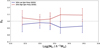 |
Fig. 6. Spin bias signal measured from the SDSS LowZ group catalog using the halo spin proxy, which is based on the SOC method. Red symbols and lines show results for the 50% higher spin proxy subset, while blue symbols and lines represent groups in the 50% lower spin proxy subset. Error computation details are provided in the text. |
To assess the significance of the aforementioned measurement, we used the following procedure. First, we obtained a bias distribution by sampling the group catalog 100 times and measuring the relative bias for each of the resulting samples. Using this technique, we created two separate distributions for the high-spin proxy and low-spin proxy subsets. Then, to assess how often the red measurements are greater than the blue measurements, we randomly sampled a red and a blue point from each distribution and recorded how often the red point was above the blue point, repeating this procedure one million times. From these one million red-blue pairs, we calculated the probability that the red points have a higher relative bias than the blue points. This is denoted as “P(Red > Blue)”.
For our entire mass range, this procedure yielded P(Red > Blue) = 0.787. For groups with masses Mh > 1013.2 h−1 M⊙, the probability rises to P(Red > Blue) = 0.850 (we recall that this is the mass range where we expect a higher correlation between our proxy and λ; see Fig. 3). For individual mass bins, we found P(Red > Blue) = 75.3%, 59.1%, 69.0%, 93.7%, and 89.8%, from low to high mass. We note that the bin widths for the SDSS LowZ group catalog measurement are larger because the sample is smaller.
It is clear that there are some differences between the results from observations and simulations. These differences are to be expected because of the inherent challenges regarding the measurement, which is influenced by fiber collisions near cluster centers and observational uncertainties in the masses of groups, to name a few. It is encouraging, however, that the high-spin proxy measurements of relative bias are consistently above the low-spin proxy results across the mass range for five independent group mass bins.
4.3. Parameter dependencies of the observational probe
In Fig. 6, we chose a set of fiducial parameters to measure spin bias, which are listed in Table 1. These were found to be effective when testing on our TNG300 mock. Here, we allow some of the parameters to vary in order to evaluate the effect on the measured spin bias and to better judge the sensitivity of the secondary bias signal to these parameters4.
The results of varying the projected radius and the scales where the cross-correlation function is computed are shown in Fig. 7. We first tried varying the range in which neighbor galaxies are identified, i.e., from 1 R200 to 3 R200 and up to 5 R200 from the halo and group (see left column). We did not observe any significant qualitative changes in the results. Next, we tried varying the range of scales over which the cross-correlation function is computed (as indicated in the figure subtitle). Once more, we did not see any significant qualitative difference between the three selections. This suggests that the measurement of spin bias based on our spin proxy is not highly sensitive to these parameter choices, at least as far as the general trend is concerned. Furthermore, the high-spin proxy sample is consistently and significantly above the low-spin proxy sample across the majority of the mass bins. It therefore appears that our results are not a special case based on fine-tuning of parameters.
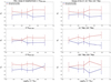 |
Fig. 7. Similar to Fig. 6 but varying the configuration parameters of our spin proxy. The left column shows the impact of varying the distance range of neighboring galaxies, while the right column displays results assuming different scale intervals for the computation of the cross-correlation function. We note that the fiducial result is shown in the top panels. |
Next, we tested the impact of varying the depth of the cylinder used to select neighbors as well as whether including all group members – as defined by the SDSS LowZ catalog (Lim et al. 2017) – affects the measurement. In the group catalog, group membership is determined by identifying the galaxies within the radius of R200 of each halo after compensating for the Fingers-of-God effect. This effect makes the distribution of galaxies inside groups in redshift space appear elongated along the line of sight. The Fingers-of-God effect is primarily caused by the peculiar motion of each galaxy within the gravitational potential of the host halo. Therefore, if we select a narrow velocity cut from the halo center velocity, as done in our fiducial setup, we exclude the galaxies with the highest peculiar velocities. However, as described in Sect. 3.1, this choice was made to concentrate on the more relaxed members of their group, which were shown to provide a stronger spin proxy signal in our mock tests. This choice also mitigates environmental effects. To evaluate the effect of this velocity cut, we tested three different values: 50, 500, and 5000 km/s.
An alternative approach would be to consider all members of the group as provided by the SDSS LowZ catalog (Lim et al. 2017). With this definition, there is a possibility of contamination from the surrounding environment. On the other hand, fiber collisions can produce incompleteness, especially in crowded fields, such as in cluster cores. To test the impact of fiber collisions, we conducted an additional test that excludes member galaxies within the inner 0.3 R200 range of each halo. The results of all these velocity and membership-related tests are presented in Fig. 8. Despite some quantitative differences in the shapes of individual trends, the general result remains unchanged, as the higher relative bias of the high-spin proxy subset is visible across all five configurations.
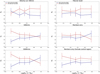 |
Fig. 8. Similar to Fig. 7 but varying the velocity cut (left column) and our membership criteria (right column). The lower-right panel shows the result of excluding galaxies within 0.3 R200 of the groups. For comparison, the fiducial result is shown in the upper-right panel. |
Additionally, we tested the impact of using group masses derived from an alternative approach, i.e., a luminosity-based method where the halo mass is traced by the central galaxy luminosity instead of galaxy mass. We again obtained similar results in terms of the general trend. This uniform outcome shows that our main result is insensitive to the particular choices of the measurement. We note, again, that differences in the mass dependence of the signal are expected given the challenges associated with this measurement.
5. Discussion
Our results demonstrate that we are on a promising path toward an observational detection of halo spin bias using the SOC method. Upcoming surveys with larger volumes and improved statistics have the potential to confirm these preliminary findings and offer new opportunities for studying secondary bias.
While these preliminary results are encouraging, there are several aspects that can contribute to limiting the significance of our results. In observations, the more the spin vector of clusters aligns with the line of sight, the harder it is to estimate neighbor motion, which obviously weakens the correlation between our spin proxy and λ. Also, cluster statistics affect the correlation function, particularly because we employed volume-limited samples. We expect that these limitations can be mitigated in upcoming galaxy surveys.
Although we only concentrated on the spin bias signal at face value, we note the possibility that other secondary parameters could also be at play and potentially contribute to any signal that is detected by the SOC method. One example is a well-known dependency of secondary bias on the local environment (e.g., Paranjape et al. 2018; Montero-Dorta & Rodriguez 2024). In the future, we hope to have sufficient statistics to allow us to control for other secondary parameters in order to cleanly investigate spin bias. We note that a secondary bias connects internal halo properties with a large-scale bias, so it is important to remove any local environmental effects that could masquerade as a secondary bias signal.
Another interesting point of discussion is that an inversion of the signal was reported in Sato-Polito et al. (2019) using the MultiDark simulations, albeit at a low halo mass, i.e., Mh ≃ 1011.5 h−1 M⊙. As our focus is mainly on the higher mass range of groups in this study, we generally did not observe this inversion. The physical origin of this low-mass behavior was subsequently revealed in Tucci et al. (2021), where the authors evaluated the effect of splashback halos on the signal. These low-mass, low-spin halos that are found close to massive halos can create an inversion of the signal. The effect of splashback halos on our analysis is an interesting aspect that could potentially be addressed in a follow-up work.
As mentioned before, it is challenging to determine if a clear dependence of spin bias on group mass exists using the current data. We note that in large-volume simulations, it has been shown that spin bias increases toward the high-mass end (i.e., the relative biases of the high- and low-spin subsets become progressively more separated). By refining our methods and including additional data sets (Tempel et al. 2017; Rodriguez & Merchán 2020; Nelson et al. 2024), we expect to be able to probe this mass dependence in the near future.
6. Summary and conclusions
It is well known that the clustering of DM halos depends primarily on halo mass. For instance, more massive halos are more tightly clustered than their less massive counterparts (Press & Schechter 1974; Sheth & Tormen 1999, 2002; Sheth et al. 2001). However, if we control for this primary effect, additional dependencies on secondary halo properties are expected to be revealed, as seen in numerical simulations (see, e.g., Sheth & Tormen 2004; Gao et al. 2005; Wechsler et al. 2006; Gao & White 2007; Angulo et al. 2008; Li et al. 2008; Faltenbacher & White 2010; Lazeyras et al. 2017; Salcedo et al. 2018; Han et al. 2019; Mao et al. 2018; Sato-Polito et al. 2019; Johnson et al. 2019; Ramakrishnan et al. 2019; Montero-Dorta et al. 2020, 2021a, 2025; Tucci et al. 2021; Montero-Dorta & Rodriguez 2024). In this work, we have presented, for the first time, a methodology to measure halo spin bias in observations, that is, the secondary dependence of halo bias on halo spin at a fixed halo mass. We tested our procedure on TNG300 cosmological simulation data and applied it to the SDSS observational data.
As the true spin of groups and clusters – the observable counterparts of halos – cannot be directly observed, we developed a spin proxy based on what we call SOC. This effect, previously studied in simulations (Kim et al. 2022), refers to the correlation between the orbital motion of neighboring galaxies – both around and within a target group – and the magnitude and direction of the group’s spin vector.
To test the feasibility of using this SOC-based spin proxy in observations, we first evaluated the performance of the proxy using a mock catalog constructed from the TNG300 simulation. We confirmed that despite the projection effects that are inherent to an observational catalog, the spin proxy displays a significant correlation with the halo spin parameter (λ). This correlation is sufficient to preserve the halo spin bias effect. In essence, halos with a higher spin proxy at a fixed halo mass have a higher bias than the halo population with a lower spin proxy. In TNG300 mock, we experimented with different configurations to optimize the methodology. The strongest signal was obtained using all host halos with total masses greater than 1012h−1 M⊙ and neighbor subhalos more massive than 109h−1 M⊙. We also only considered neighbors within 1 R200 of the host halo, and we measured the spin bias from the cross-correlation function over a range of scales between 5 and 15 h−1 Mpc.
Given the promising outcome with the mocks, the next step of our analysis was to apply our methodology to an observational catalog. We used the SDSS LowZ sample (Lim et al. 2017) in combination with the Yang et al. (2005) group catalog. As in TNG300 mock, we split groups based on the spin proxy and measured their relative bias at a fixed group mass. We reported indications of spin bias across the entire mass range considered. For the most massive groups (log10(Mh[h−1 M⊙]) ≳ 13), we measured a significance of 85%. This value was obtained by randomly sampling the bias measurement of the high- and low-spin proxy subsets within each mass bin. In 85% of the cases, the higher spin proxy subset has a higher relative bias.
With future data sets, this methodology could provide the first observational detection of halo spin bias. Moreover, a future study using this methodology would be one of the first claims of secondary halo bias detection (see, e.g., Miyatake et al. 2016; Lin et al. 2016; Montero-Dorta et al. 2017; Niemiec et al. 2018; Sunayama et al. 2022; Obuljen et al. 2020; Salcedo et al. 2022; Wang et al. 2022 for more context). Importantly, we verified that our results are not too sensitive to changes in the parameters that define the proxy, such as the distance range for neighbors, the scales employed in the correlation function estimation, and other choices.
Our pioneering study opens up several new research avenues. The spin bias measurement can potentially be used as a new cosmological test. This research line could be strengthened if the same measurement is performed in other spectroscopic data sets at higher redshift so that the evolution of the spin-bias signal can be determined. Furthermore, measuring the halo spin for a sizable sample of clusters and groups would allow us to study how these systems gain spin and how this process depends on the cosmic web. Our long-term goal is to use this work as a foundation for future endeavors to bridge the gap between internal halo properties and their surrounding environments over diverse scales.
For reference, these cuts correspond to ∼2500 and 25 DM particles, respectively.
Throughout this work, “central halo” refers to the host halo, while “neighboring galaxies” can either be satellites of that host or other galaxies in its vicinity.
It is important to bear in mind that given the challenges involved and the pioneering nature of this analysis, our primary goal is to assess whether a general trend with the spin proxy exists. Therefore, reproducing the exact shape of the spin bias is beyond the scope of this paper.
Acknowledgments
Yigon Kim has supported by National Research Foundation of Korea (NRF), through grants funded by the Korean government (MSIT) (Nos. 2022R1A4A3031306), during this work. Yigon also thanks Kyungpook National University SPHEREx Basic Research Lab and Seoul National University ExgalCos group for their kind support. Antonio D. Montero-Dorta thanks Fondecyt for financial support through the Fondecyt Regular 2021 grant 1210612. Rory Smith acknowledges financial support from FONDECYT Regular 2023 project No. 1230441 and also gratefully acknowledges financial support from ANID – MILENIO NCN2024_112.
References
- Albareti, F. D., Allende Prieto, C., Almeida, A., et al. 2017, ApJS, 233, 25 [Google Scholar]
- Angulo, R. E., Baugh, C. M., & Lacey, C. G. 2008, MNRAS, 387, 921 [NASA ADS] [CrossRef] [Google Scholar]
- Barnes, J., & Efstathiou, G. 1987, ApJ, 319, 575 [NASA ADS] [CrossRef] [Google Scholar]
- Bell, E. F., McIntosh, D. H., Katz, N., & Weinberg, M. D. 2003, ApJS, 149, 289 [Google Scholar]
- Bullock, J. S., Dekel, A., Kolatt, T. S., et al. 2001, ApJ, 555, 240 [NASA ADS] [CrossRef] [Google Scholar]
- Dalal, N., White, M., Bond, J. R., & Shirokov, A. 2008, ApJ, 687, 12 [NASA ADS] [CrossRef] [Google Scholar]
- Faltenbacher, A., & White, S. D. M. 2010, ApJ, 708, 469 [NASA ADS] [CrossRef] [Google Scholar]
- Gao, L., & White, S. D. M. 2007, MNRAS, 377, L5 [NASA ADS] [CrossRef] [Google Scholar]
- Gao, L., Springel, V., & White, S. D. M. 2005, MNRAS, 363, L66 [NASA ADS] [CrossRef] [Google Scholar]
- Genel, S., Vogelsberger, M., Springel, V., et al. 2014, MNRAS, 445, 175 [Google Scholar]
- Han, J., Li, Y., Jing, Y., et al. 2019, MNRAS, 482, 1900 [NASA ADS] [CrossRef] [Google Scholar]
- Johnson, J. W., Maller, A. H., Berlind, A. A., Sinha, M., & Holley-Bockelmann, J. K. 2019, MNRAS, 486, 1156 [CrossRef] [Google Scholar]
- Kim, Y., Smith, R., & Shin, J. 2022, ApJ, 935, 71 [Google Scholar]
- Landy, S. D., & Szalay, A. S. 1993, ApJ, 412, 64 [Google Scholar]
- Lazeyras, T., Musso, M., & Schmidt, F. 2017, JCAP, 2017, 059 [Google Scholar]
- Lee, J. H., Pak, M., Lee, H.-R., & Song, H. 2019a, ApJ, 872, 78 [Google Scholar]
- Lee, J. H., Pak, M., Song, H., et al. 2019b, ApJ, 884, 104 [Google Scholar]
- Li, Y., Mo, H. J., & Gao, L. 2008, MNRAS, 389, 1419 [NASA ADS] [CrossRef] [Google Scholar]
- Lim, S. H., Mo, H. J., Lu, Y., Wang, H., & Yang, X. 2017, MNRAS, 470, 2982 [NASA ADS] [CrossRef] [Google Scholar]
- Lin, Y.-T., Mandelbaum, R., Huang, Y.-H., et al. 2016, ApJ, 819, 119 [NASA ADS] [CrossRef] [Google Scholar]
- Mao, Y.-Y., Zentner, A. R., & Wechsler, R. H. 2018, MNRAS, 474, 5143 [NASA ADS] [CrossRef] [Google Scholar]
- Marinacci, F., Vogelsberger, M., Pakmor, R., et al. 2018, MNRAS, 480, 5113 [NASA ADS] [Google Scholar]
- Miyatake, H., More, S., Takada, M., et al. 2016, Phys. Rev. Lett., 116, 041301 [NASA ADS] [CrossRef] [Google Scholar]
- Mo, H. J., & White, S. D. M. 1996, MNRAS, 282, 347 [Google Scholar]
- Montero-Dorta, A. D. 2021, Boletin de la Asociacion Argentina de Astronomia La Plata Argentina, 62, 159 [Google Scholar]
- Montero-Dorta, A. D., & Rodriguez, F. 2024, MNRAS, 531, 290 [NASA ADS] [CrossRef] [Google Scholar]
- Montero-Dorta, A. D., Pérez, E., Prada, F., et al. 2017, ApJ, 848, L2 [NASA ADS] [CrossRef] [Google Scholar]
- Montero-Dorta, A. D., Artale, M. C., Abramo, L. R., et al. 2020, MNRAS, 496, 1182 [NASA ADS] [CrossRef] [Google Scholar]
- Montero-Dorta, A. D., Chaves-Montero, J., Artale, M. C., & Favole, G. 2021a, MNRAS, 508, 940 [NASA ADS] [CrossRef] [Google Scholar]
- Montero-Dorta, A. D., Artale, M. C., Abramo, L. R., & Tucci, B. 2021b, MNRAS, 504, 4568 [Google Scholar]
- Montero-Dorta, A. D., Contreras, S., Artale, M. Celeste, Rodriguez, F., & Favole, G. 2025, A&A, 695, A159 [NASA ADS] [CrossRef] [EDP Sciences] [Google Scholar]
- Mroczkowski, T., Nagai, D., Basu, K., et al. 2019, Space Sci. Rev., 215, 17 [Google Scholar]
- Naiman, J. P., Pillepich, A., Springel, V., et al. 2018, MNRAS, 477, 1206 [Google Scholar]
- Nelson, D., Pillepich, A., Springel, V., et al. 2018, MNRAS, 475, 624 [Google Scholar]
- Nelson, D., Springel, V., Pillepich, A., et al. 2019, Comput. Astrophys. Cosmol., 6, 2 [Google Scholar]
- Nelson, D., Pillepich, A., Ayromlou, M., et al. 2024, A&A, 686, A157 [NASA ADS] [CrossRef] [EDP Sciences] [Google Scholar]
- Niemiec, A., Jullo, E., Montero-Dorta, A. D., et al. 2018, MNRAS, 477, L1 [NASA ADS] [CrossRef] [Google Scholar]
- Obuljen, A., Percival, W. J., & Dalal, N. 2020, JCAP, 2020, 058 [CrossRef] [Google Scholar]
- Paranjape, A., Hahn, O., & Sheth, R. K. 2018, MNRAS, 476, 3631 [NASA ADS] [CrossRef] [Google Scholar]
- Pasquali, A., Smith, R., Gallazzi, A., et al. 2019, MNRAS, 484, 1702 [Google Scholar]
- Peebles, P. J. E. 1969, ApJ, 155, 393 [Google Scholar]
- Pillepich, A., Nelson, D., Hernquist, L., et al. 2018a, MNRAS, 475, 648 [Google Scholar]
- Pillepich, A., Springel, V., Nelson, D., et al. 2018b, MNRAS, 473, 4077 [Google Scholar]
- Planck Collaboration XIII. 2016, A&A, 594, A13 [NASA ADS] [CrossRef] [EDP Sciences] [Google Scholar]
- Press, W. H., & Schechter, P. 1974, ApJ, 187, 425 [Google Scholar]
- Ramakrishnan, S., Paranjape, A., Hahn, O., & Sheth, R. K. 2019, MNRAS, 489, 2977 [NASA ADS] [CrossRef] [Google Scholar]
- Rodriguez, F., & Merchán, M. 2020, A&A, 636, A61 [NASA ADS] [CrossRef] [EDP Sciences] [Google Scholar]
- Salcedo, A. N., Maller, A. H., Berlind, A. A., et al. 2018, MNRAS, 475, 4411 [NASA ADS] [CrossRef] [Google Scholar]
- Salcedo, A. N., Zu, Y., Zhang, Y., et al. 2022, Sci. China Phys. Mech. Astron., 65, 109811 [Google Scholar]
- Sánchez, S. F., Kennicutt, R. C., Gil de Paz, A., et al. 2012, A&A, 538, A8 [Google Scholar]
- Sánchez, S. F., García-Benito, R., Zibetti, S., et al. 2016, A&A, 594, A36 [Google Scholar]
- Sato-Polito, G., Montero-Dorta, A. D., Abramo, L. R., Prada, F., & Klypin, A. 2019, MNRAS, 487, 1570 [NASA ADS] [CrossRef] [Google Scholar]
- Sheth, R. K., & Tormen, G. 1999, MNRAS, 308, 119 [Google Scholar]
- Sheth, R. K., & Tormen, G. 2002, MNRAS, 329, 61 [Google Scholar]
- Sheth, R. K., & Tormen, G. 2004, MNRAS, 350, 1385 [NASA ADS] [CrossRef] [Google Scholar]
- Sheth, R. K., Mo, H. J., & Tormen, G. 2001, MNRAS, 323, 1 [NASA ADS] [CrossRef] [Google Scholar]
- Sinha, M., & Garrison, L. H. 2020, MNRAS, 491, 3022 [Google Scholar]
- Springel, V. 2010, MNRAS, 401, 791 [Google Scholar]
- Springel, V., Pakmor, R., Pillepich, A., et al. 2018, MNRAS, 475, 676 [Google Scholar]
- Sunayama, T., More, S., & Miyatake, H. 2022, ArXiv e-prints [arXiv:2205.03277] [Google Scholar]
- Tempel, E., Tuvikene, T., Kipper, R., & Libeskind, N. I. 2017, A&A, 602, A100 [NASA ADS] [CrossRef] [EDP Sciences] [Google Scholar]
- Tucci, B., Montero-Dorta, A. D., Abramo, L. R., Sato-Polito, G., & Artale, M. C. 2021, MNRAS, 500, 2777 [Google Scholar]
- Vogelsberger, M., Genel, S., Springel, V., et al. 2014a, MNRAS, 444, 1518 [Google Scholar]
- Vogelsberger, M., Genel, S., Springel, V., et al. 2014b, Nature, 509, 177 [Google Scholar]
- Walcher, C. J., Wisotzki, L., Bekeraité, S., et al. 2014, A&A, 569, A1 [NASA ADS] [CrossRef] [EDP Sciences] [Google Scholar]
- Wang, K., Mao, Y.-Y., Zentner, A. R., et al. 2022, MNRAS, 516, 4003 [Google Scholar]
- Wechsler, R. H., Zentner, A. R., Bullock, J. S., Kravtsov, A. V., & Allgood, B. 2006, ApJ, 652, 71 [NASA ADS] [CrossRef] [Google Scholar]
- White, S. D. M., & Frenk, C. S. 1991, ApJ, 379, 52 [Google Scholar]
- White, S. D. M., & Rees, M. J. 1978, MNRAS, 183, 341 [Google Scholar]
- Yang, X., Mo, H. J., van den Bosch, F. C., & Jing, Y. P. 2005, MNRAS, 356, 1293 [Google Scholar]
All Tables
Fiducial configuration for the spin bias measurement in the SDSS LowZ group catalog.
All Figures
|
Fig. 1. Stellar mass (M*) versus redshift for galaxies in the SDSS LowZ catalog. Black markers show the entire sample, while the red markers show our volume-limited sample. |
| In the text | |
|
Fig. 2. Simplified illustration of the concept behind spin proxy based on SOC and its measurement. Illustration 1 depicts the SOC itself, while illustrations 2 and 3 show how the spin direction is determined by identifying the direction in which the coherence signal is strongest. |
| In the text | |
|
Fig. 3. Correlation between the spin proxy and the true halo spin (λ) for several host halo mass bins in TNG300. The solid lines show the mean of the distribution, while the shaded regions indicate the interquartile range (25th to 75th percentiles). These measurements have been performed in 3D. |
| In the text | |
|
Fig. 4. Cross-correlation function of the SDSS LowZ group catalog as a function of group mass. The group mass range (log(Mh/h−1 M⊙)) of each measurement is indicated in the legend. As predicted from theory, more massive groups are more strongly clustered, which is the primary dependency of halo bias. |
| In the text | |
|
Fig. 5. Halo spin bias measured in projection from the TNG300 mock. Higher spin and higher spin proxy measurements are shown in orange and red solid lines and symbols, while the lower spin and lower spin proxy measurements are represented by cyan and blue solid lines, respectively. (See text for information regarding the computation of errors.) |
| In the text | |
|
Fig. 6. Spin bias signal measured from the SDSS LowZ group catalog using the halo spin proxy, which is based on the SOC method. Red symbols and lines show results for the 50% higher spin proxy subset, while blue symbols and lines represent groups in the 50% lower spin proxy subset. Error computation details are provided in the text. |
| In the text | |
|
Fig. 7. Similar to Fig. 6 but varying the configuration parameters of our spin proxy. The left column shows the impact of varying the distance range of neighboring galaxies, while the right column displays results assuming different scale intervals for the computation of the cross-correlation function. We note that the fiducial result is shown in the top panels. |
| In the text | |
|
Fig. 8. Similar to Fig. 7 but varying the velocity cut (left column) and our membership criteria (right column). The lower-right panel shows the result of excluding galaxies within 0.3 R200 of the groups. For comparison, the fiducial result is shown in the upper-right panel. |
| In the text | |
Current usage metrics show cumulative count of Article Views (full-text article views including HTML views, PDF and ePub downloads, according to the available data) and Abstracts Views on Vision4Press platform.
Data correspond to usage on the plateform after 2015. The current usage metrics is available 48-96 hours after online publication and is updated daily on week days.
Initial download of the metrics may take a while.