| Issue |
A&A
Volume 700, August 2025
|
|
|---|---|---|
| Article Number | L3 | |
| Number of page(s) | 6 | |
| Section | Letters to the Editor | |
| DOI | https://doi.org/10.1051/0004-6361/202555364 | |
| Published online | 31 July 2025 | |
Letter to the Editor
Insights into chromospheric large-scale flows using Nobeyama 17 GHz radio observations
I. The differential rotation profile
1
Aryabhatta Research Institute of Observational Sciences, Nainital, 263002 Uttarakhand, India
2
Department of Applied Physics, Mahatma Jyotiba Phule Rohilkhand University, Bareilly, 243006 Uttar Pradesh, India
3
Department of Physics, University of Helsinki, P.O. Box 64, FI-00014 Helsinki, Finland
4
Udaipur Solar Observatory, Physical Research Laboratory, Dewali, Badi Road, Udaipur, 313 001 Rajasthan, India
5
Department of Physics, Ahmednagar College, Station Road, Ahilyanagar, 414001 Maharashtra, India
6
Indian Institute of Space Science and Technology, Valiamala, Thiruvananthapuram, 695 547 Kerala, India
7
Indian Institute of Astrophysics, Koramangala, Bangalore, 560034, India
8
Center of Excellence in Space Sciences India, IISER Kolkata, Mohanpur, 741246 West Bengal, India
⋆ Corresponding author: This email address is being protected from spambots. You need JavaScript enabled to view it.
Received:
2
May
2025
Accepted:
3
July
2025
Abstract
Context. Although the differential rotation rate on the solar surface has long been studied using optical and extreme ultraviolet (EUV) observations, associating these measurements with specific atmospheric heights remains challenging due to the temperature-dependent emission of tracers observed in EUV wavelengths. Radio observations, being primarily influenced by coherent plasma processes and/or thermal bremsstrahlung, offer a more height-stable diagnostic and thus provide an independent means to test and validate rotational trends observed at other EUV wavelengths.
Aims. We aim to characterise the differential rotation profile of the upper chromosphere using cleaned solar full-disc 17 GHz radio imaging from the Nobeyama Radioheliograph spanning a little over two solar cycles (1992–2020).
Methods. A tracer-independent method based on automated image correlation was employed on daily full-disc 17 GHz radio maps. This method determines the angular velocities in 16 latitudinal bins of 15° each by maximising the 2D cross-correlation of overlapping image segments.
Results. The best-fit parameters for the differential rotation profile are A = 14.520 ± 0.006°/day, B = –1.443 ± 0.099°/day, and C =–0.433 ± 0.267°/day. These results suggest that the upper chromosphere rotates significantly faster than the photosphere at all latitudes, with a relatively flatter latitudinal profile. We also observed a very weak anti-correlation, ρs = −0.383 (94.73%), between the equatorial rotation rate and solar activity.
Conclusions. Our findings reaffirm the potential of radio observations to probe the dynamics of the solar chromosphere with reduced height ambiguity. The overlap of the equatorial rotation rate (A) found in this study with that for 304 Å in the EUV regime lends additional support to the view that the equatorial rotation rates increase with height above the photosphere. Future coordinated studies at wavelengths with better-constrained height formation will be crucial for further understanding the complex dynamics of the solar atmosphere.
Key words: plasmas / Sun: activity / Sun: chromosphere / Sun: general / Sun: radio radiation / Sun: rotation
© The Authors 2025
 Open Access article, published by EDP Sciences, under the terms of the Creative Commons Attribution License (https://creativecommons.org/licenses/by/4.0), which permits unrestricted use, distribution, and reproduction in any medium, provided the original work is properly cited.
This article is published in open access under the Subscribe to Open model. This email address is being protected from spambots. You need JavaScript enabled to view it. to support open access publication.
1. Introduction
Large-scale flows on the Sun play a pivotal role in shaping the global dynamics of the solar atmosphere and influence the distribution of magnetic fields across various layers of the solar interior and exterior. Among these flows, differential rotation, is one of the most fundamental and extensively studied global motions of the Sun, and it has been observed not only at the solar surface but across the full extent of the solar atmosphere. This phenomenon is formulated empirically using the following equation,
 (1)
(1)
The differential rotation of the solar photosphere has been widely studied through feature tracking, flux modulation, and other methods (e.g. Newton & Nunn 1951; Snodgrass 1983). Furthermore, recent advancements in helioseismology have significantly enhanced understanding of the latitudinal and radial rotation profiles within the solar interior (Antia et al. 1998, 2008). With growing observational capabilities spanning optical, ultraviolet (UV), extreme ultraviolet (EUV), and radio wavelengths, the opportunity has emerged to reframe the phenomenon of differential rotation in the Sun in terms of a broader class of large-scale flows that pervade the atmosphere. From this perspective, differential rotation is not merely a parameterisation of latitudinal shear but a tracer of how angular momentum transport, plasma motions, and magnetic fields are coupled across spatial and temporal scales in the solaratmosphere.
Despite centuries of investigation, the nature of how such flows evolve with height and temperature and their interconnection across stratified atmospheric layers remains incompletely understood due to the height ambiguity of tracers involved in the extraction of the differential rotation profile. Recent studies, particularly those using the Atmospheric Imaging Assembly (AIA) on board the Solar Dynamic Observatory (SDO; e.g. Sharma et al. 2020; Routh et al. 2024), have demonstrated that a possible connection between the rotation rate of the solar atmosphere might exist with height above the photosphere. These trends suggest that the atmospheric layers are not passively rotating but may be dynamically linked to deeper processes that are possibly governed by the magnetic field topology. This line of reasoning has found support in works that compare atmospheric rotation with internal rotation profiles derived from helioseismology (e.g. Badalyan 2010; Finley & Brun 2023), thus hinting at connections mediated by magnetically anchored structures.
Despite such broad research efforts, the phenomenon of differential rotation has been difficult to grasp in the upper and hotter solar atmosphere for various reasons, including but not limited to the fast-changing nature of higher atmospheric tracers as well as the height ascribed to them. Although the faster rotation of the hotter solar atmosphere, specifically the chromosphere, has long been suggested through different methods and different datasets (Livingston 1969; Mishra et al. 2024; Routh et al. 2024), an ambiguity in the exact height of the origin of the emission dataset in such studies has always left a gap to be fulfilled. Extending this inquiry into radio wavelengths offers an even less ambiguous insight into the chromosphere, transition region, and corona. Radio observations, such as those from the Nobeyama Radioheliograph (NoRH), provide height-stable diagnostics of the upper chromosphere and transition region (e.g. 34 and 17 GHz emission (8.8 and 17.6 mm, respectively); Selhorst et al. 2008), thereby avoiding the temperature-based ambiguities that often affect EUV diagnostics. In an attempt to address this gap, this study utilises a tracer-independent method to ascertain the spatial and temporal variation in the differential rotation of the solar atmosphere at well-defined heights above the photosphere as determined from radio emission.
The article is arranged as follows. In Section 2 we discuss the observations and data analysis method, and Section 3 provides a discussion of the results. Finally, in Section 4 we summarise the present work and discuss the conclusion.
2. Observation and data analysis
2.1. The Nobeyama Radioheliograph
The NoRH, operational from 1992 July until 2020 March, observed the solar chromosphere and the transition region at frequencies of 34 and 17 GHz, respectively, at a resolution of 10″ (Nakajima et al. 1994). The cleaned solar full-disc images1 used in this study have dimensions of 512 × 512 pixel2 with a pixel scale of 4.91″. These images are image registered and aligned such that solar north coincides with the image north.
2.2. Data pre-processing and method of image correlation
Since the image data of the cleaned solar full-disc fits from NoRH primarily represent the brightness temperature of various features in the solar atmosphere, the maximum brightness temperature values in the dataset can vary significantly depending on the observed solar activities (Selhorst et al. 2003). This might create an issue regarding the method of image correlation, which primarily utilises the intensity gradient information to minimise the brightness conservation or the optical flow equation (Neggers et al. 2016). To get rid of this spuriousness in the data, the entire dataset was first minmax-scaled (see Fig. 1b) such that the scaled brightness of each pixel i in the dataset is given by the following equation:
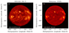 |
Fig. 1. Sun from (a) a space-based perspective as seen by AIA atop SDO and (b) a ground-based perspective as seen by the NoRH. |
 (2)
(2)
Here, Bmin and Bmax are the minimum and maximum brightness of the entire dataset. This step ensures the entire dataset has brightness values of ∈ [0, 1], thereby standardising the dataset. The resulting dataset was then subjected to a method of image correlation similar to that outlined in Mishra et al. (2024) and Routh et al. (2024) to obtain the sidereal rotation rate (Ωθ) corresponding to the maximum correlation coefficient in each latitudinal bin. A brief description of the method is discussed in Appendix A.
3. Results and discussion
After setting a threshold on the value of the cross-correlation coefficient to ensure the integrity of the analysis statistics (a detailed discussion of this approach and further examination of this technique is available in Mishra et al. 2024; Routh et al. 2024), an average (Ωθ) weighted by the corresponding cross-correlation coefficient in each latitudinal bin was obtained for each latitude (θ). The uncertainty of these values was then determined as a combination of the standard statistical error (σSSE) and the least count error2. These values were subsequently fitted to Eq. (1) using the Levenberg-Marquardt least square (LMLS; Markwardt 2009) method to obtain the best-fit parameters A, B, and C and the respective uncertainty (ΔA, ΔB, and ΔC) in determining them. Thereafter, we obtained the values A + ΔA = 14.520 ± 0.006 ° /day, B + ΔB = −1.443 ± 0.099 ° /day, and C + ΔC = −0.433 ± 0.267 ° /day (Fig. 2) for the solar chromosphere as seen at a frequency of 17 GHz.
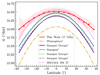 |
Fig. 2. Rotation profile of solar chromosphere as obtained from 17 GHz data from NoRH data when compared with rotational profiles from 1Snodgrass (1983, 1984), 2Howard et al. (1984), 3Poljančić Beljan et al. (2017), 4Ruždjak et al. (2017), 5Jha et al. (2021), and 6Routh et al. (2024). |
Upon examining Fig. 2, it is immediately apparent that the rotational profile is significantly higher than that of the photospheric plasma and sunspot groups, and it is also relatively flatter, indicating that the solar chromosphere at a height of 3000 ± 500 km above the solar visible surface rotates more rapidly than the underlying photosphere at all latitudes, which is similar to the findings by Chandra et al. (2009) using three years of NoRH data. It is also evident that the rotational profile displays a relatively flatter trend, suggesting a reduced differential nature. This result aligns well with the rotational profile of the chromosphere from SDO/AIA 304 Å (Routh et al. 2024), which samples plasma in the temperature range of log10T = 4.7 K (Lemen et al. 2012) and supposedly represents a height of 2820 ± 400 km (Kwon et al. 2010) above the photosphere. Additionally, these findings are consistent with several studies, such as Li et al. (2020), Mishra et al. (2024), that utilised spectroheliogram data from both space- and ground-based data probing different parts of the solar chromosphere. The results for A obtained in this study also conform to the existing trend for the equatorial rotation rate at different heights in the solar atmosphere, as suggested by previous studies (as shown in Fig. 3).
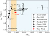 |
Fig. 3. Variation in equatorial rotation rate from the photosphere to different parts of the corona from recent works. The umbrella label of ‘sunspots’ is demarcated with an asterisk (*) to indicate different datasets used by different studies (see Appendix B). The extents of different layers of the solar atmosphere are shaded differently (photosphere in grey, chromosphere in gold, and corona in light blue) to allow distinction between the same. The heights representing the different temperature sensitive filters have been taken from Sanjay et al. (2024) (for 131 Å only) and the references in Routh et al. (2024). The representative height for 17 GHz has been obtained from Zirin (1988). The error bars along y represent a 3σ variation in the parameters, while along x the error bars represent the exact variation reported in the mentioned studies. A detailed table compiling all values in this figure and several other studies are available for reference in Appendix B. |
We then looked at the variation of the rotational parameters with respect to the strength of the solar cycle, as designated by sunspot number. From a correlation analyses involving the Spearman correlation coefficient (ρs) to explore any potential monotonous relationship, we found that both the equatorial rotation rate (A) and the latitudinal gradient (B) exhibit little to no significant relationship with solar activity (Fig. 4). This observation is consistent with such previous studies as Bertello et al. (2020), Mishra et al. (2024), Routh et al. (2024). However, upon closer inspection, a very weak negative correlation for A (ρs = −0.4 (94.72%)) with solar activity strength was observed, aligning with Brajša et al. (2006), Li et al. (2023), but no such relationship was evident for B (ρs = −0.11 (39.25%)).
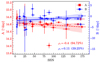 |
Fig. 4. Correlation plot of equatorial rotation rate (A; in red) and latitudinal gradient (B; in blue) with the yearly sunspot number and their error estimate in the y and x directions, respectively. The lines of best fit are exhibited to visualise the generalised trend in the correlation. The shaded regions with each line correspond to the confidence interval of the fit. |
4. Summary and conclusions
We have analyzed 28 years of radio imaging data from the Nobeyama Radio Observatory to examine the differential rotation profile of the upper chromosphere using an automated image correlation technique3. The distinguishing factor of this method is the fact that unlike the tracer method, which depends heavily on the availability of a singular feature distinguished by intensity, the method of image correlation is sensitive to only intensity gradients in each pixel and does not depend heavily on the availability of dominant features. This ensures that even during minima periods, a proper shift is identified based only on the intensities of each pixel in a bin. However, this also allows for the rotational profiles of several prominent features such as coronal holes, filaments, and active regions to coexist without being differentiated. A numerical analysis to differentiate the contribution of these features may be attempted in the future, but it is out of the scope of this particular study. Our goal in this study was to associate the derived rotational profile with a specific height in the upper solar atmosphere, reducing the ambiguity often encountered with EUV observations, which are typically sensitive to particular temperatures, leading to greater uncertainty regarding the representative height above the photosphere, as higher atmospheric features of similar temperature range may also contribute to the filter-recorded intensity. Our findings indicate that the solar atmosphere at a height of 3000 ± 500 km rotates significantly faster than the photosphere below and shares similar rotational characteristics with 304 Å from SDO/AIA. This agreement of parameters obtained from a temperature sensitive channel, which can include contributions from features at different heights reaching log10T = 4.7 K locally, is within the 3σ range (Fig. 3) with values derived from radio emissions, which predominantly originate from a single height (Selhorst et al. 2008; Oliveira e Silva et al. 2016). Such an agreement reduces ambiguity in the possibility that there is a genuine upward trend in the solar atmosphere with increasing height. It is also worth noting that the overlap of the equatorial rotation rate (A) found in this study with that for 304 Å, which in turn matches the A obtained for a depth of r = 0.94 R⊙ (Routh et al. 2024), may further support the idea that magnetic features in the higher solar atmosphere have footpoints deep into the convection zone (e.g. Weber 1969; Mancuso et al. 2020, and references therein).
An investigation into the impact of solar activity strength on the parameters A and B revealed that neither parameter is significantly affected, although a very weak negative correlation was observed for A, in agreement with Li et al. (2013), Jurdana-Šepić et al. (2011), Ruždjak et al. (2017), Wan & Gao (2022). This result may be understood in light of the numerical simulations explored by Brun (2004), Brun et al. (2004), whose results suggest that a subtle deceleration in differential rotation may be attributed to Maxwell stresses opposing Reynolds stresses, leading to reduced differential rotation. A similar result was obtained analytically by Lanza (2006; 2007) for young late-type stars. However, this inference should be taken with caution, as the correlation coefficient and its confidence level are too weak to draw any definitive conclusions.
This study’s findings contribute to our understanding of the complex relationship between solar rotation and atmospheric height by decreasing the ambiguity associated with the representative height associated with the observed rotational profile of higher solar atmosphere that has long been explored using optical, UV, and EUV wavelengths. Further studies exploring coronal counterparts in wavelengths where height determination is less ambiguous could provide stronger confidence in the trend of the rotation rate so consistently observed and thereby explore the mechanisms behind the observed rotational characteristics and their implications for solar dynamics. Additionally, long-term monitoring of these parameters could provide insights into potential changes in solar rotation over extended periods and as to why barely any impact of solar activity is seen on the chromospheric rotational rate, which may have further implications for solar activity cycles and space weather predictions.
σLCE = 0.1°.
The generalised code is available for open source use at: https://github.com/srinjana-routh/Image-Correlation
This analysis is performed using https://hesperia.gsfc.nasa.gov/ssw/gen/idllibs/astron/image/correlimages.pro available in the SolarSoftWare library in Interactive Data Language (IDL)
The generalised code is available for open source use at https://github.com/srinjana-routh/Bright-Regions-Nobeyama
Acknowledgments
S.R. is supported by funding from the Department of Science and Technology (DST), Government of India, through the Aryabhatta Research Institute of Observational Sciences (ARIES). The computational resources utilised in this study were provided by ARIES. AK acknowledges the ANRF Prime Minister Early Career Research Grant (PM ECRG) program. The data utilised in this work havee been acquired from the Nobeyama Radio Observatory (NRO) database. All the authors are grateful to the observers at NRO for the data. Yearly mean sunspot numbers come from the source: WDC-SILSO, Royal Observatory of Belgium, Brussels, and these can be downloaded from https://www.sidc.be/silso/.
References
- Antia, H. M., Basu, S., & Chitre, S. M. 1998, MNRAS, 298, 543 [Google Scholar]
- Antia, H. M., Basu, S., & Chitre, S. M. 2008, ApJ, 681, 680 [Google Scholar]
- Badalyan, O. G. 2010, New Astron., 15, 135 [NASA ADS] [CrossRef] [Google Scholar]
- Balthasar, H., Vazquez, M., & Woehl, H. 1986, A&A, 155, 87 [Google Scholar]
- Bertello, L., Pevtsov, A. A., & Ulrich, R. K. 2020, ApJ, 897, 181 [NASA ADS] [CrossRef] [Google Scholar]
- Brajša, R., Ruždjak, D., & Wöhl, H. 2006, Sol. Phys., 237, 365 [CrossRef] [Google Scholar]
- Brun, A. S. 2004, Sol. Phys., 220, 333 [NASA ADS] [CrossRef] [Google Scholar]
- Brun, A. S., Miesch, M. S., & Toomre, J. 2004, ApJ, 614, 1073 [Google Scholar]
- Chandra, S., Vats, H. O., & Iyer, K. N. 2009, MNRAS, 400, L34 [NASA ADS] [Google Scholar]
- Chatterjee, S., Banerjee, D., & Ravindra, B. 2016, ApJ, 827, 87 [NASA ADS] [CrossRef] [Google Scholar]
- Finley, A. J., & Brun, A. S. 2023, A&A, 679, A29 [NASA ADS] [CrossRef] [EDP Sciences] [Google Scholar]
- Gupta, S. S., Sivaraman, K. R., & Howard, R. F. 1999, Sol. Phys., 188, 225 [NASA ADS] [CrossRef] [Google Scholar]
- Howard, R., Gilman, P. I., & Gilman, P. A. 1984, ApJ, 283, 373 [NASA ADS] [CrossRef] [Google Scholar]
- Howard, R. F., Gupta, S., & Sivaraman, K. 1999, Sol. Phys., 186, 25 [Google Scholar]
- Jha, B. K., Priyadarshi, A., Mandal, S., Chatterjee, S., & Banerjee, D. 2021, Sol. Phys., 296, 25 [Google Scholar]
- Jurdana-Šepić, R., Brajša, R., Wöhl, H., et al. 2011, A&A, 534, A17 [NASA ADS] [CrossRef] [EDP Sciences] [Google Scholar]
- Kwon, R.-Y., Chae, J., & Zhang, J. 2010, ApJ, 714, 130 [Google Scholar]
- Lanza, A. F. 2006, MNRAS, 373, 819 [NASA ADS] [CrossRef] [Google Scholar]
- Lanza, A. F. 2007, A&A, 471, 1011 [NASA ADS] [CrossRef] [EDP Sciences] [Google Scholar]
- Lemen, J. R., Title, A. M., Akin, D. J., et al. 2012, Sol. Phys., 275, 17 [Google Scholar]
- Li, K., Shi, X. J., Xie, J., et al. 2013, MNRAS, 433, 521 [Google Scholar]
- Li, K. J., Xu, J. C., Xie, J. L., & Feng, W. 2020, ApJ, 905, L11 [Google Scholar]
- Li, K. J., Wan, M., & Feng, W. 2023, MNRAS, 520, 5928 [Google Scholar]
- Livingston, W. C. 1969, Sol. Phys., 9, 448 [NASA ADS] [CrossRef] [Google Scholar]
- Mancuso, S., Giordano, S., Barghini, D., & Telloni, D. 2020, A&A, 644, A18 [NASA ADS] [CrossRef] [EDP Sciences] [Google Scholar]
- Markwardt, C. B. 2009, in Astronomical Data Analysis Software and Systems XVIII, eds. D. A. Bohlender, D. Durand, & P. Dowler, Astronomical Society of the Pacific Conference Series, 411, 251 [Google Scholar]
- Mishra, D. K., Routh, S., Jha, B. K., et al. 2024, ApJ, 961, 40 [Google Scholar]
- Nakajima, H., Nishio, M., Enome, S., et al. 1994, IEEE Proc., 82, 705 [NASA ADS] [CrossRef] [Google Scholar]
- Neggers, J., Blaysat, B., Hoefnagels, J. J., & Geers, M. M. 2016, Int. J. Numer. Methods Eng., 105, 243 [Google Scholar]
- Newton, H. W., & Nunn, M. L. 1951, MNRAS, 111, 413 [NASA ADS] [Google Scholar]
- Oliveira e Silva, A. J., Selhorst, C. L., Simões, P. J. A., & Giménez de Castro, C.~G. 2016, A&A, 592, A91 [NASA ADS] [CrossRef] [EDP Sciences] [Google Scholar]
- Poljančić Beljan, I., Jurdana-Šepić, R., Brajša, R., et al. 2017, A&A, 606, A72 [NASA ADS] [CrossRef] [EDP Sciences] [Google Scholar]
- Roša, D., Brajša, R., Vršnak, B., & Wöhl, H. 1995, Sol. Phys., 159, 393 [CrossRef] [Google Scholar]
- Routh, S., Jha, B. K., Mishra, D. K., et al. 2024, ApJ, 975, 158 [Google Scholar]
- Ruždjak, D., Ruždjak, V., Brajša, R., & Wöhl, H. 2004, Sol. Phys., 221, 225 [Google Scholar]
- Ruždjak, D., Brajša, R., Sudar, D., Skokić, I., & Poljančić Beljan, I. 2017, Sol. Phys., 292, 179 [Google Scholar]
- Sanjay, Y., Krishna Prasad, S., Erdélyi, R., et al. 2024, ApJ, 975, 236 [NASA ADS] [CrossRef] [Google Scholar]
- Selhorst, C. L., Silva, A. V. R., Costa, J. E. R., & Shibasaki, K. 2003, A&A, 401, 1143 [NASA ADS] [CrossRef] [EDP Sciences] [Google Scholar]
- Selhorst, C. L., Silva-Válio, A., & Costa, J. E. R. 2008, A&A, 488, 1079 [NASA ADS] [CrossRef] [EDP Sciences] [Google Scholar]
- Sharma, J., Kumar, B., Malik, A. K., & Vats, H. O. 2020, MNRAS, 492, 5391 [NASA ADS] [CrossRef] [Google Scholar]
- Skokić, I., Brajša, R., Roša, D., Hržina, D., & Wöhl, H. 2014, Sol. Phys., 289, 1471 [CrossRef] [Google Scholar]
- Snodgrass, H. B. 1983, ApJ, 270, 288 [NASA ADS] [CrossRef] [Google Scholar]
- Snodgrass, H. B. 1984, Sol. Phys., 94, 13 [NASA ADS] [CrossRef] [Google Scholar]
- Sudar, D., Brajša, R., Skokić, I., & Benz, A. O. 2019, Sol. Phys., 294, 163 [NASA ADS] [CrossRef] [Google Scholar]
- Wan, M., & Gao, P.-X. 2022, ApJ, 939, 111 [Google Scholar]
- Weber, E. J. 1969, Sol. Phys., 9, 150 [Google Scholar]
- Wittmann, A. D. 1996, Sol. Phys., 168, 211 [Google Scholar]
- Zirin, H. 1988, Astrophysics of the Sun (Cambridge University Press) [Google Scholar]
Appendix A: Segmentation and correlation analysis of the radio images
A.1. Method of image correlation
At a time a single pair of images, temporally separated by a day (Δt ≤ 1), are studied. These pair of images are first projected onto the heliographic grid 1800 × 1800 in dimension (0.1° along longitude and latitude; see Fig. A.1(left panel)).
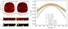 |
Fig. A.1. Left panel: Naobeyama images on (a) 7 March 2014 and (b) 8 March 2014 after the conversion to Stonyhurst heliographic coordinates. Green rectangular boxes depict the bins B1 and B2 (−20° to −5° in latitude, ±45° in longitude) used for image correlation. Bins T1 and T2 depict the dominant bright features in the same bins identified by adaptive intensity thresholding. Right panel: Rotational profiles for Nobeyama 17 GHz data using initial values from 1Ruždjak et al. (2017) and 2Poljančić Beljan et al. (2017) compared with the results using the same from 3Jha et al. (2021) and the values from 4Routh et al. (2024). Shaded areas denote uncertainties, detailed in section 3. |
The result was then divided into 16 overlapping bins of size 15° and stride of 5° in the latitudinal direction, spanning ±45° in latitude. Since there exists a centre-to-limb variation in intensity which might affect our measurement of the longitudinal shift, the longitudinal span of these bins were restricted to ±45°, thereby close to the disc centre where the effects of centre-to-limb variation is minimal (see for e.g. Sudar et al. (2019) and references therein). At a time, bins of the same latitudinal extent temporally separated by 1 day (B1 and B2 in Fig. A.1) are subjected to the method of image correlation. In this method, one bin is shifted with respect to the other bin within the range of Δϕ ∈ Δϕ0 ± 3° and Δθ ∈ Δθ0 ± 1° in longitudinal and latitudinal directions, respectively4. The initial guesses (Δθ0, Δϕ0) were calculated from the rotation rate of sunspot groups (Jha et al. 2021). An analysis locating the maximum of the resulting 2D correlation coefficient gives the value of the longitudinal shift (Δϕ), as dictated by the dominant features, when present in the given latitudinal bin (see T1 and T2 in Fig. A.1; the method of segmentation of these features are discussed in subsection A.1). This value is then utilised to obtain the synodic value of Ω ( ) at the mid-latitude θm of the same latitudinal bin. To incorporate the effect of the motion of the Earth around the Sun, we apply the sidereal correction (Roša et al. 1995; Wittmann 1996; Skokić et al. 2014; Mishra et al. 2024) on the synodic rotation rate to get the sidereal rotation rate (Ωθ , which is used in the further analyses. A detailed discussion of this method is available in Mishra et al. (2024).
A.2. Rotational profile estimates for different initial guesses.
The entire analysis was re-run with different initial values from Poljančić Beljan et al. (2017), Ruždjak et al. (2004) and compared with the original analysis, where initial values were taken from Jha et al. (2021) to see if the initial guesses contributed to any significant change in the rotational profiles thus obtained. As can be seen in Fig. A.1(right panel), all the rotational profiles obtained overlap and there is no significant change even when the initial guesses obtained from the three depicted studies vary significantly (see Table A.1).
Rotation parameters for Nobeyama 17 GHz data obtained using different initial guesses.
A.3. Segmenting large-scale features
To accentuate the understanding of the contribution of different features at different temperatures (or heights), an image segmentation method based on adaptive intensity thresholding was designed for the bright regions (e.g, active regions) (T1 and T2 in Fig. A.1). This was achieved by using the mean method for adaptive thresholding (Chatterjee et al. 2016) to a smoothed and histogram-equalised image5 and is given by
 (A.1)
(A.1)
where Iij is the intensity value of the ijth pixel, μdisc is the mean, σdisc is the standard deviation of the solar disc and k (=1, here) is a scalar that can be adjusted based on the attribute we aim to segment. This method segments even small-scale brightenings which might correspond to coronal hole regions as well. An additional area threshold of 120.6 arcsec2 (≈63.38 × 10⁶ km2), determined using trial-and-error method, was applied to discard any spurious brightening that might be of non-physical origin and extract large-scale features that remained for the exemplar latitudinal bin.
Appendix B: Rotation parameters of different parts and features of the solar atmosphere compiled from relevant studies
Some rotation parameters of different features and parts of the solar atmosphere as obtained through various studies.
All Tables
Rotation parameters for Nobeyama 17 GHz data obtained using different initial guesses.
Some rotation parameters of different features and parts of the solar atmosphere as obtained through various studies.
All Figures
|
Fig. 1. Sun from (a) a space-based perspective as seen by AIA atop SDO and (b) a ground-based perspective as seen by the NoRH. |
| In the text | |
|
Fig. 2. Rotation profile of solar chromosphere as obtained from 17 GHz data from NoRH data when compared with rotational profiles from 1Snodgrass (1983, 1984), 2Howard et al. (1984), 3Poljančić Beljan et al. (2017), 4Ruždjak et al. (2017), 5Jha et al. (2021), and 6Routh et al. (2024). |
| In the text | |
|
Fig. 3. Variation in equatorial rotation rate from the photosphere to different parts of the corona from recent works. The umbrella label of ‘sunspots’ is demarcated with an asterisk (*) to indicate different datasets used by different studies (see Appendix B). The extents of different layers of the solar atmosphere are shaded differently (photosphere in grey, chromosphere in gold, and corona in light blue) to allow distinction between the same. The heights representing the different temperature sensitive filters have been taken from Sanjay et al. (2024) (for 131 Å only) and the references in Routh et al. (2024). The representative height for 17 GHz has been obtained from Zirin (1988). The error bars along y represent a 3σ variation in the parameters, while along x the error bars represent the exact variation reported in the mentioned studies. A detailed table compiling all values in this figure and several other studies are available for reference in Appendix B. |
| In the text | |
|
Fig. 4. Correlation plot of equatorial rotation rate (A; in red) and latitudinal gradient (B; in blue) with the yearly sunspot number and their error estimate in the y and x directions, respectively. The lines of best fit are exhibited to visualise the generalised trend in the correlation. The shaded regions with each line correspond to the confidence interval of the fit. |
| In the text | |
|
Fig. A.1. Left panel: Naobeyama images on (a) 7 March 2014 and (b) 8 March 2014 after the conversion to Stonyhurst heliographic coordinates. Green rectangular boxes depict the bins B1 and B2 (−20° to −5° in latitude, ±45° in longitude) used for image correlation. Bins T1 and T2 depict the dominant bright features in the same bins identified by adaptive intensity thresholding. Right panel: Rotational profiles for Nobeyama 17 GHz data using initial values from 1Ruždjak et al. (2017) and 2Poljančić Beljan et al. (2017) compared with the results using the same from 3Jha et al. (2021) and the values from 4Routh et al. (2024). Shaded areas denote uncertainties, detailed in section 3. |
| In the text | |
Current usage metrics show cumulative count of Article Views (full-text article views including HTML views, PDF and ePub downloads, according to the available data) and Abstracts Views on Vision4Press platform.
Data correspond to usage on the plateform after 2015. The current usage metrics is available 48-96 hours after online publication and is updated daily on week days.
Initial download of the metrics may take a while.