| Issue |
A&A
Volume 700, August 2025
|
|
|---|---|---|
| Article Number | A230 | |
| Number of page(s) | 13 | |
| Section | Astrophysical processes | |
| DOI | https://doi.org/10.1051/0004-6361/202555427 | |
| Published online | 25 August 2025 | |
A disturbance in the force
How force fluctuations hinder dynamical friction and induce core stalling
1
Consiglio Nazionale delle Ricerche, Istituto dei Sistemi Complessi, via Madonna del Piano 17, 50022 Sesto Fiorentino (FI), Italy
2
INFN – Sezione di Firenze, via G. Sansone 1, 50022 Sesto Fiorentino (FI), Italy
3
INAF – Osservatorio Astrofisico di Arcetri, Largo E. Fermi 5, 50125 Firenze, Italy
4
Laboratoire J.-A. Dieudonné, UMR 6621, Université Côte d’Azur, Parc Valrose, 06108 Nice Cedex 02, France
5
Departamento de Estructura de la Materia, Física Térmica y Electrónica, Universidad Complutense Madrid, 28040 Madrid, Spain
⋆ Corresponding authors: This email address is being protected from spambots. You need JavaScript enabled to view it.
; This email address is being protected from spambots. You need JavaScript enabled to view it.
Received:
7
May
2025
Accepted:
15
July
2025
Abstract
Context. Dynamical friction is an important phenomenon in stellar dynamics (and plasma physics) resulting in the slowing down of a massive test particle upon many two-body scatters with background particles. Chandrasekhar’s original formulation, developed for idealized infinite and homogeneous systems, has been found to be sufficiently accurate even in models of finite extent and radially dependent density profiles. However, in some cases N-body simulations have evidenced a breakdown of Chandrasekhar’s formalism. In particular, in the case of cored stellar systems, the analytical predictions underestimate the rate of in-fall of the test particle. Moreover, the orbital decay appears to stop at a critical radius where in principle the effect of dynamical friction should still be non-negligible.
Aims. Several explanations for such discrepancy have been proposed so far. In spite of this, it remains unclear whether the origin is a finite N effect or an effect arising from the resonance (or near-resonance) of the orbits of the test and field particles, which is independent of N, such as dynamical buoyancy. Here we aim to shed some light on this issue with tailored numerical experiments.
Methods. We performed ad hoc simulations of a massive tracer initially placed on a low-eccentricity orbit in spherical equilibrium models with increasing resolution. We used an N-body code for which the self-consistent interaction among the background particles can be substituted with the effect of the static smooth potential of the system’s continuum limit, so that the higher-order contributions to the dynamical friction arising from the formation of a wake can be neglected if needed.
Results. We find that, contrary to what has been reported in previous literature, a suppression of dynamical friction happens in both cuspy and cored models. When neglecting the interaction among field particles, we observe in both cases a clear N−1/2 scaling of the radius at which dynamical friction ceases to be effective. This hints at a granularity-induced origin of the so-called core-stalling of the massive tracer in cored models.
Key words: instabilities / methods: numerical / galaxies: kinematics and dynamics / galaxies: star clusters: general
© The Authors 2025
 Open Access article, published by EDP Sciences, under the terms of the Creative Commons Attribution License (https://creativecommons.org/licenses/by/4.0), which permits unrestricted use, distribution, and reproduction in any medium, provided the original work is properly cited.
This article is published in open access under the Subscribe to Open model. This email address is being protected from spambots. You need JavaScript enabled to view it. to support open access publication.
1. Introduction
Dynamical friction (hereafter DF, Chandrasekhar 1943a,b,c) is the process that drives a massive particle of mass mt, for example a compact object (black hole, neutron star) or a satellite dwarf galaxy, to sink into the host stellar system via multiple dynamical collisions with its constituting field particles of (mean) mass m. In its original formulation, evaluated for an infinitely extended system of constant number and mass density, n, and ρ = mn with isotropic velocity distribution f(v), DF amounts to a velocity dependent drag term of the form
 (1)
(1)
In the equation above, lnΛ is the (velocity averaged) Coulomb logarithm of the maximum to minimum impact parameters, Λ = bmax/bmin, in the hyperbolic scattering with 1/r2 forces, v = ||v||, and
 (2)
(2)
is the fractional velocity volume function (e.g. see Ciotti 2021) that counts the portion of field particles moving slower than mt and contributing to DF.
Since its inception, Equation (1) has been applied with success to a wide plethora of astrophysical system ranging from massive stars in globular clusters (GCs) to satellite galaxies in dark matter (DM) halos. However, numerical experiments have so far revealed that a naive correction to the Chandrasekhar expression, whereby essentially one substitutes the local values of ρ(r) and f(v) in Eq. (1), might lead to either an overestimation or underestimation of DF. For example, in a series of papers also accounting for the feedback of mt on the host system by Bertin et al. (2003), Arena et al. (2006), Arena & Bertin (2007), it has been shown that the classical idealized DF formulation works rather well in models with broad density cores, while it fails (i.e. predicts shorter sinking timescales) when the density profile is highly concentrated at small radii. In addition, in the latter case the feedback on the density distribution is less and less important the higher its initial concentration. Conversely, Read et al. (2006) and Goerdt et al. (2006, 2010) observed that massive objects moving on initially circular orbits in cored models first suffer a stronger DF, with respect to the Chandrasekhar estimate – often referred to as super-Chandrasekhar – to then ‘stall’ at a radius, rs, which appears to depend on the specific details of the galaxy model and on mt. This apparent suppression of DF1 in stellar (or DM) cores, frequently dubbed core-stalling, has also been reported among others by Zelnikov & Kuskov (2016) for satellites sinking in flat galactic cores, by Kaur & Sridhar (2018), Dutta Chowdhury et al. (2019), and Cole et al. (2012), Bílek et al. (2024) in simulations of GCs orbiting dwarf galaxies, and by Genina et al. (2024) in simulations of supermassive black holes (SMBHs) in nuclear star clusters.
Banik & van den Bosch (2021, 2022) (see also Dattathri et al. 2025) interpret the core-stalling (at least in very weakly collisional systems) as an effect of the Lynden-Bell & Kalnajs (1972) torque generalized such that its original secular and adiabatic assumptions are relaxed to account for the contribution of the non-resonant orbits to the slowing down of the massive test particle. In practice once the test particle reaches the central core, the structure of the relative orbits of the near-resonant field particles, m, with respect to mt (e.g. see Inoue 2011) changes significantly. Since the phase space distribution in nearly harmonic cores is characterized by rather gentle gradients, the net torque from said orbits is statistically almost always positive, thereby countering the friction (an effect labeled as dynamical buoyancy). The core-stalling is therefore happening once the torque induced buoyancy balances DF. Remarkably, another resonance-based argument (see Tremaine & Weinberg 1984), which was sketched out by Read et al. (2006) but later ruled out by Petts et al. (2015, 2016), interpreted the so-called super-Chandrasekhar regime observed in some N-body simulations as a consequence of using a local Maxwellian approximation to evaluate Ξ(v), instead of integrating over the phase-space distribution, f, which supports the specific density profile of the host model (see Appendix A, see also Kazantzidis et al. 2004).
For the tightly related problem of a heavy particle (BH) initially sitting at rest at the centre of a flat-cored system then migrating outwards due to the combined action of force fluctuations and torques2, N-body simulations (e.g. Chatterjee et al. 2002a,b, 2003; Brockamp et al. 2011; Di Cintio et al. 2023) revealed a strong resolution dependence of the wander radius, rwan (Bahcall & Wolf 1976), loosely defined as the typical displacement of mt from the centre of the potential well, in the form
 (3)
(3)
where rc is the typical scale length of the model, M its total mass, and N the number of stars (or simulation particles in a N-body experiment). Another radial scale considered in BH dynamics that is usually compared with rwan is the so-called influence radius (i.e. the radius below which the potential, Φt = −Gmt/r, exerted by mt dominates over the contribution of the host stellar system, e.g. see Peebles 1972), defined as
 (4)
(4)
where σ is the velocity dispersion. This established, it remains unclear whether, at least in some regimes of N and mt, the core stalling is a discreteness effect linked to the rapid and incoherent force fluctuations in dense cores, or a resolution-independent process related to the instantaneous fraction of orbits with frequencies nearly resonant with the test particle mt. In this work we explore this matter further by means of variable resolution N-body simulations and single particle propagation in smooth potentials with tunable DF and mean force fluctuations.
2. Setting the stage
2.1. Galaxy models
In most of the simulations discussed in this paper, we employ the frequently used γ models (Dehnen 1993; Tremaine et al. 1994) with a density distribution defined by
 (5)
(5)
generating the gravitational potential
![Mathematical equation: $$ \begin{aligned} \Phi (r)=\frac{GM}{r_c}\times {\left\{ \begin{array}{ll} \displaystyle \frac{1}{(2-\gamma )}\left[\left(\frac{r}{r+r_c}\right)^{2-\gamma }-1\right]\quad \mathrm{for}\quad \gamma \ne 2.\\ \displaystyle \ln \frac{r}{r+r_c} \quad \mathrm{for}\quad \gamma =2. \end{array}\right.} \end{aligned} $$](/articles/aa/full_html/2025/08/aa55427-25/aa55427-25-eq6.gif) (6)
(6)
The parameter γ appearing in Eqs. (5) and (6) above controls the central logarithmic density slope, ranging from 0 (corresponding to a flat core) to 3 (corresponding to a singularity). Here we concentrate on the cored γ = 0 and mildly cuspy γ = 1 cases. When generating the simulations initial conditions, the radial coordinates, ri, of the N field particles are obtained sampling ρ with the usual Monte Carlo technique applied to the radial mass profile,
 (7)
(7)
while their angular positions, ϑi and φi, are assigned randomly from two independent uniform distributions. The modulus of the velocities, vi, is assigned using the rejection method (for example, see Di Cintio et al. 2015 and references therein) to sample the isotropic equilibrium phase-space distribution,
 (8)
(8)
where Ψ = −Φ and ℰ = Ψ − v2/2 are the relative potential and energy, respectively, and
![Mathematical equation: $$ \begin{aligned} y\left(\Psi \right)= {\left\{ \begin{array}{ll} \displaystyle \left[1-(2-\gamma )\Psi \right]^{1/(2-\gamma )},\quad \gamma \ne 2.\\ \displaystyle \exp \left(-\Psi \right),\quad \gamma =2. \end{array}\right.} \end{aligned} $$](/articles/aa/full_html/2025/08/aa55427-25/aa55427-25-eq9.gif) (9)
(9)
In addition, to compare with previous numerical work, we have also considered the simpler Plummer (1911) model defined by the density potential pair
 (10)
(10)
with the radial mass profile
 (11)
(11)
The isotropic phase-space distribution function associated with the model (10) is
 (12)
(12)
where  is the central velocity dispersion. We note that the radial gravitational accelerations of ar = −GM(r)/r2 in the Plummer model and the γ = 0 model are both nearly harmonic near their centres; however, for the same choice of M and rc, the radial span over which ar ∝ r is larger for the Plummer density profile.
2.2. N-body method and simulation set-up
We performed N-body simulations in which a test mass, mt, sinked in an equilibrium system represented by N equal mass m = M/N field particles, with 104 ≤ N ≤ 3 × 10⁶. The test particle mass values used in this work range from 2 × 10⁻⁴ to 10−2 in units of the total mass of the host system, M, while the orbit of mt is initialized with values of the eccentricity, e, ranging from 0 (i.e. circular orbit) to 0.9, corresponding to a relatively eccentric orbit. As usual e is defined as
 (13)
(13)
where rapo and rperi are the apocentre and pericentre of the unperturbed orbit in the smooth potential, Φ.
In our numerical experiments the field particles either interact with each other, with forces computed with the fast Dehnen (2000) tree scheme implemented in the FVFPS code (see Londrillo et al. 2003; Nipoti et al. 2006), or move as independent tracers in the smooth potential given by Eqs. (6), (10) in a similar fashion to White (1983) and Bontekoe & van Albada (1987). In this latter case, we aim to neglect the higher-order effects on DF induced by the formation of a self-gravitating wake (Mulder 1983; Kaur & Stone 2022) behind mt, sometimes also referred to as a polarization cloud (Gilbert 1970; Kalnajs 1972; Heyvaerts et al. 2017). In both types of simulation, each field particle of mass m interacts with the test particle, mt, with the gravitational force evaluated with a direct sum scheme. To prevent unwanted resolution-induced force singularities, the Newtonian 1/r2 interaction is substituted with a quadratic spline below the softening length, ϵ. In the results discussed hereafter, the fixed choice was ϵ = 2 × 10⁻³rc. We recall that in direct and tree codes the softening acts as a sort of spatial resolution. We recall also that the introduction of said softening effectively dictates a fixed minimum impact parameter in two body-encounters (see Huang et al. 1993; Chiron & Marcos 2019). All particles are propagated with a second-order leapfrog scheme with a fixed time step, Δt = tc/150, where the reference timescale is  . We adopted units such that G = M = rc = tc = 1.
2.3. Stochastic equation of motion models
For reference we also performed simulations where mt is propagated in the smooth potential under the additional effect of DF and force fluctuations modeling the ‘granularity’ of the system, in principle with an arbitrary resolution, without resulting to integrating the field particle orbits. In practice, following the approach of Sartorello et al. (2025) we assume that the dynamics of mt is statistically equivalent to that induced by the stochastic differential Langevin equation (see Chandrasekhar 1943d; Kandrup 1980)
 (14)
(14)
where ηv is essentially the DF term given in Eq. (1) and δf is a stochastic force (per unit mass) fluctuation. The formulation of the problem given by Eq. (14) is equivalent to the evolution equation for the particle energy fluctuations ⟨dE/dt⟩ derived by Bekenstein & Maoz (1992) and Maoz (1993) for homogeneous or inhomogeneous gravitational media using a fluctuation-dissipation approach.
In the case of an infinite and homogeneous system of equal mass particles interacting via 1/r2 forces subjected to Poissonian density fluctuations, δf is distributed according (see Chandrasekhar & von Neumann 1942, 1943) to the Holtsmark (1919) distribution, originally evaluated for an infinite gas of charged particles. The Holtsmark distribution of the modulus of the force fluctuations, δf = ||δf||, reads in integral form as a function of the dimensionless auxiliary variable, s, as
![Mathematical equation: $$ \begin{aligned} \mathcal{F} (\delta f)=\frac{2}{\pi \delta f}\int _0^\infty \exp \left[-\alpha (s/\delta f)^{3/2}\right]s\sin (s)\mathrm{d}s, \end{aligned} $$](/articles/aa/full_html/2025/08/aa55427-25/aa55427-25-eq17.gif) (15)
(15)
while its density dependent normalization factor, α, is defined as
 (16)
(16)
Consistently with previous work, we accommodated the definition (15) in the γ models (5) and Plummer model (10) using the local values of ρ (e.g. see Petrovskaya 1986) and used the typical local Maxwellian approximation3 for the velocity distribution of the model in the Chandrasekhar formula so that
![Mathematical equation: $$ \begin{aligned} \Xi (v)=(4\pi )^{-1}\left[\mathrm{Erf}\left(\frac{v}{\sqrt{2}\sigma }\right)-\sqrt{\frac{2}{\pi }}\frac{v}{\sigma }\exp \left(-\frac{v^2}{2\sigma ^2}\right)\right]. \end{aligned} $$](/articles/aa/full_html/2025/08/aa55427-25/aa55427-25-eq19.gif) (17)
(17)
For the γ models, the radial velocity dispersion profile is given in an integral form as
 (18)
(18)
In the two cases of interest explored here, γ = 0 and 1, we have
 (19)
(19)
and (see also Hernquist 1990)
![Mathematical equation: $$ \begin{aligned} \sigma ^2(r)&=\frac{GM}{12r_c}\bigg [\frac{12r(r+r_c)^3}{r_c^4}\ln \bigg (\frac{r+r_c}{r}\bigg )+\nonumber \\&\quad -\frac{r}{r+r_c}\bigg (25+\frac{52r}{r_c}+\frac{42r^2}{r_c^2}+\frac{12r^3}{r_c^3}\bigg )\bigg ], \end{aligned} $$](/articles/aa/full_html/2025/08/aa55427-25/aa55427-25-eq22.gif) (20)
(20)
respectively, while for the Plummer sphere we have
 (21)
(21)
The Coulomb logarithm appearing in Eq. (1) was evaluated accounting for the exact integration over the impact parameter, b, in hyperbolic orbits (see e.g. Binney & Tremaine 2008) as
![Mathematical equation: $$ \begin{aligned} \log \bigg [1+\bigg (\frac{b_{\rm max}}{b_{\rm min}}\bigg )^2\bigg ]=\log \bigg \{1+\bigg [\frac{r_* \sigma ^2}{G(m_t+m)}\bigg ]^2\bigg \}\approx \log \Lambda . \end{aligned} $$](/articles/aa/full_html/2025/08/aa55427-25/aa55427-25-eq24.gif) (22)
(22)
The choice of minimum impact parameter, bmin, was made as usual to account for the angular momentum conservation in a φ = π/2 deflection at relative velocity of the order of the local velocity dispersion, σ, while bmax was set to r*, a typical scale length of the order of the average inter-particle distance, ⟨r⟩=(8πmrc3/3M)1/3 ∝ rc/N1/3. We stress the fact that there is still not much of a consensus around the ‘correct’ choice of bmax (see Hamilton et al. 2018), with some authors assuming the scale length of the host, rc, and others (e.g. Kandrup 1980, 1983) preferring the local average interparticle distance,  (see the discussion in van Albada & Szomoru 2020). Another choice could be the distance at which the correlations in the fluctuations of stellar density, velocity, and gravitational potential induced by mt vanish, in a similar fashion to the Debye-Hukel theory in neutral plasmas (see Marochnik 1968). Ad hoc direct N-body simulations by Marcos et al. (2017), in which bmin can be artificially fixed by the softening parameter, ϵ, seem to indicate that bmax ≈ rc/3. Here we note that, due to their rather low highest resolution (i.e. N ≈ 1.7 × 10⁴), setting the maximum impact parameter to either rc/3 or ⟨r⟩ inside the logarithm has little effect on the magnitude of the DF coefficient for resolutions below roughly ∼5 × 10⁶.
The stochastic equation of motion (14) was solved by computing the DF term at all times as a function of the local density and velocity distribution of the background model, and sampling the modulus of the force fluctuations from Eq. (15) with a standard Monte Carlo. The direction of the fluctuations was assumed to be isotropic (i.e. δf was given a random direction by sampling a uniform distribution of angles). We integrated Eq. (14) with the generalized leapfrog scheme implemented in Pasquato & Di Cintio (2020), Di Cintio et al. (2020), Sartorello et al. (2025) (for additional details and the original implementation see also Mannella 2004; Burrage et al. 2007). The benefits of applying this integration technique are essentially the fact that it converges on the standard second-order Verlet scheme for vanishing noise and friction, and its rather fast convergence on asymptotic distributions in the case of simple Brownian motion. Other higher-order and time-adaptive schemes, for example Runge-Kutta or Bulrisch-Stoer (see Burrage et al. 2007), require longer computational times, as is dictated by a smaller adaptive Δt, to obtain a comparable accuracy. It must be pointed out that the method introduced by Mannella (2004) in our implementation explicitly assumes a delta-correlated noise (i.e. subsequent encounters are independent); however, strictly speaking, it must be noted that the space-integrated force fluctuations are at zero-sum altogether, since δf is related to density fluctuations, δρ, through the usual Poisson equation. At constant total mass, all fluctuations must integrate out to zero. This implies that force fluctuations cannot be completely uncorrelated, making the delta-correlated noise a rough approximation that could be, in principle, sharpened by introducing a correlation time, τc (see e.g. Trani & Di Cintio 2025). Other authors, such as Pogorelov & Kandrup (1999) and Terzic & Kandrup (2003), used different forms of the correlation function of gravitational fluctuations, without finding significant qualitative differences with the delta-correlated noise in the case of strongly interacting systems. In some runs, in which the δf term was artificially set to zero, we instead used a modified mid-point leapfrog, typically adopted for the integration of orbits with velocity-dependent force terms (see for example Mikkola & Merritt 2006).
2.4. Recovering the distribution of force fluctuations
Using a locally tailored Holtsmark distribution in Eq. (14) might seem a rather crude approximation. In order to check the reliability of this assumption, inspired by previous work by Ahmad & Cohen (1973, 1974) and Del Popolo (1996a,b) we studied the numerically evaluated distribution of the force (per unit mass) fluctuations for some discrete N-body realization of the models discussed in the previous section.
We defined the force fluctuation at the position ri of the ith particle in a discrete realization of the parent continuum system as
 (23)
(23)
where Φ is the smooth potential given by Eq. (5) or Eq. (10), with normalization such that M = Nm. We then partitioned the model in Ns logarithmically spaced radial shells and evaluated for each of them the probability density function, 𝒫, of the modulus of the force fluctuations, δf = ||δf||, by particle counts as well as its average value, ⟨δf⟩, and variance,  . In Fig. 1 we show ⟨δf⟩ (left) and
  (right) for a Plummer model with N = 106 for Ns = 20 radial shells as a function of their radius, r. It appears that both the average and the variance of the force fluctuations grow for decreasing r, being almost constant inside the core (i.e. below rc). The associated histograms of 𝒫(δf) are shown in Fig. 2 for 100 independent realizations (grey dots) and their average (blue dots), together with the Holtsmark distribution (red lines) computed evaluating numerically the integral in Eq. (15) with the choice of α where m = M/N and ρ = ρ(r) for the specific model at hand, in this case given by Eq. (10). Remarkably, the empirical force distribution4 appears to agree rather well with the Holtsmark distribution, in particular for the shells enclosing larger fractions of N for which the different realizations have a less pronounced scatter -the average number of field particles,
  , in each shell is indicated at the bottom of the panels, so that we can safely assume that the stochastic single particle simulations can be reasonably compared to honest direct N-body simulations, at least for what concerns the form of the fluctuation distribution.
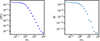 |
Fig. 1. Radial profile of the average of the discrete force fluctuations (left panel) and its variance (right panel) evaluated for a single realization of a Plummer system with N = 106. |
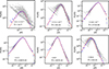 |
Fig. 2. Numerically evaluated distribution of force fluctuation, 𝒫(δf), in different shells of increasing radius (clockwise from top left, r = 3.1 × 10⁻², 7.2 × 10⁻², 0.38, 1.3, 6.9, and 54.8 in units of rc) for a Plummer model with N = 106 and 102 realizations (grey dots). The blue dots mark the PDF averaged over said ensemble, while the red curve is the corresponding the Holtsmark distribution (15) computed for the local value of the density, ρ(r), and average number of particles in the shell, |

3. Simulations and results
3.1. Preliminary tests
As a first set of numerical experiments, we compared the orbital decay of the test mass, mt, in self-consistent N-body simulations and non-interacting tracer systems, for different resolutions and initial orbital eccentricities. We find that, in both cases, independently of the specific model or details of the orbit, the core-stalling can always be observed to some degree. For a given combination of initial orbital parameters and galaxy model, the same mass, mt, systematically reaches a slightly smaller stalling radius, rs, in the simulation, where it is slowed down by non-interacting tracers. In the simulations discussed hereafter, rs is estimated by time-averaging the radial position of mt over the last 10tc of the simulation. Additionally we have also evaluated the PDF of the radial position over the same time span and extracted its mean and standard deviation, finding a rather good agreement with the time average. Overall, the orbital decay is qualitatively comparable across the two types of runs, first affecting only ra. As an example, in Fig. 3 we show two test orbits with initial eccentricities of e = 0.001 and 0.3, for a particle of mass mt = 10−3M propagated in γ = 0 and γ = 1 models (left and right panels, respectively). Both orbits plotted here stall at a rs larger than the softening length, ϵ = 2 × 10⁻³rc, used in the simulation, here indicated by the horizontal dashed line. Typically, the orbit begins to stall (i.e. the decrease in the pericentre becomes faster than that of the apocentre) once the enclosed mass fraction, M(r), becomes of the same order as mt, as is indicated by the dotted black lines. The critical radius, rmt, where this happens encloses a systematically smaller number of particles for decreasing N. Therefore for the low-resolution cases it may contain only order 10 particles. A further comparison between the two sets of numerical experiments is discussed in Appendix B.
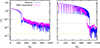 |
Fig. 3. Radial decay of a massive tracer, mt = 10−3M, orbiting in a γ = 0 (left) and a γ = 1 (right) model in a self consistent N-body run (blue curves) and a simplified simulation where the same N = 106 field particles move independently in the static smooth potential (magenta curves). The horizontal dashed orange line marks the value of the softening parameter ϵ = 2 × 10⁻³rc, while the dotted black line indicates the radius, rmt, at which M(r) = mt, equal to ≈0.1 for the simulations with γ = 0 and ≈0.033 for those with γ = 1. |
As a means to explore the feedback of mt on the parent system, in Fig. 4 we plot the radial density profile, ρ(r) at t = 103tc (triangles), against the initial one (squares), corresponding to the simulations shown in Fig. 3. In the case of the cored system (γ = 0, top panel), ρ shows little to no evolution in both self-consistent (upward blue triangles) and non-interacting tracer (downward magenta triangles) runs. A small departure from the analytical profile around r ≈ 10−2rc can be rather unambiguously interpreted as resolution effects as they decrease for higher resolutions and increase for lower ones (here N = 106). Test particles, mt, sinking in cuspy models appear to affect to a larger degree the density profile of the host system once reaching their inner regions, an effect that is related to the so-called BH scouring in elliptical galaxies hosting single or binary SMBHs (e.g. see Nasim et al. 2021 and references therein). In practice, strong scatters between stars on radial orbits and the massive BH deplete the stellar density profile, reducing the slope of a possibly initially steeper stellar cusp. In the simulations performed here (see bottom panel of Fig. 4, and the related inset), we observe a substantial depletion of the central cusp of the γ = 1 model in the simulation with non-interacting tracers, and an almost complete suppression of the cusp for the self-consistent case, where the background system becomes effectively ‘cored’ as in the N-body simulations reported by Goerdt et al. (2010).
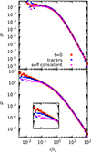 |
Fig. 4. Initial density profile corresponding to a γ = 0 (top) and a γ = 1 (bottom) model (filled orange squares) and corresponding density profiles at t = 103tc in the self-consistent and tracers in smooth potential simulations (upward blue triangles and downward magenta triangles, respectively). The dashed black lines mark ρ(r) as given in Eq. (5). The points correspond to the same simulations of Fig. 3. |
Prompted by the good agreement between the theoretical Holtsmark distribution for an infinite system with the force fluctuation distribution in spherical shells on a finite model (cfr. Fig. 2), it is natural to compare the orbital decay of a test mass in a N-body simulation with the trajectory of the same mass in the corresponding system modeled by Eq. (14). We performed several runs for different values of mt/M and choices of the density profile, ρ, finding that, in general, the stochastic equation method acceptably recovers both the timescale over which the mean galactocentric distance of given test mass halves and, in the case of a cored model, its stalling radius, rs. As an example, Figure 5 shows the evolution of r/rc for a test particle, mt = 3 × 10⁻³M, initially placed on a nearly circular orbit at r = 2rc in a Plummer model with N = 106, propagated in a N-body simulation (magenta curve) and in a stochastic simulation (cyan curve). For comparison, we also added the orbital decay evaluated adding the Chandrasekhar DF (1) to the smooth potential without fluctuations (dashed black line). In agreement with the literature discussed above, we observe that mt stalls at around rs ≈ 0.25rc, with the N-body simulation always remaining in a sub-Chandrasekhar regime. Notably, at variance with the DF-only integration, where the particle falls to the centre of the Plummer system remaining on approximately circular orbits of decaying radius, in both the N-body and the stochastic simulations some finite change in eccentricity (more marked for the orbit obtained integrating Eq. (14)) can be appreciated.
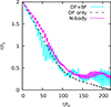 |
Fig. 5. Decay of the galactocentric distance in a Plummer system for a particle with mt = 2 × 10⁻³M in a N-body simulation with N = 106 (magenta curve), and two semi-analytical integrations in the parent smooth potential with DF and fluctuations (solid cyan line) and with DF only (dashed black line). |
3.2. N-body simulations
We investigated the resolution-induced partial suppression of DF by evolving the same initial condition for the test particle, mt, in different realizations of γ models with an increasing number of particles, N, and fixed total mass, M. In the interval 104 ≤ N ≤ 3 × 10⁶, for each explored value of mt in the range between 2 × 10⁻⁴ and 10−2 in units of M, the stalling radius, rs, systematically settles at lower values for increasing N. We observe that, at fixed N and mt and initial orbital parameters e and a, the stalling radius is always lower in models with a central cusp, in both self-consistent and simplified N-body simulations with tracers.
In Fig. 6 we show rs/rc as a function of N for cored and cuspy γ models for mt = 10−3M initially placed on nearly circular orbits with the semi-major axis a ≈ 2rc. We find that the stalling radius decreases with N, with a rather robust  trend, as is indicated by the dashed line. The square root tendency is indicative of a discreteness effect-related mechanism behind the core-stalling (e.g. see Gabrielli et al. 2014; El-Zant et al. 2019, and references therein). This becomes even more evident if the evolution of the galactocentric distance of the different realizations is rescaled by the estimated value of rs times N1/2. In Figure 7 we show the decay of rs up to t = 103tc in a γ = 0 (top) and γ = 1 (bottom) model for the case of mt = 10−3M in a system of non-interacting tracers and the associated rescaled curves for the last 50tc (left panels). A good data collapse is obtained, as also the amplitude of the fluctuations of rs fall on the same scale with a N−1/2 trend (middle panels in Fig. 7). A similar picture was also recovered for the self-consistent simulations (not shown here).
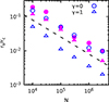 |
Fig. 6. Core-stalling radius as function of N for a particle of mass mt = 10−3M in a cored model (γ = 0, circles) and a mildly cuspy model (γ = 1, triangles). Filled magenta symbols refer to the full self-consistent N-body simulations, and empty blue ones to the simulations with non-interacting tracers. To guide the eye, the dashed line marks the N−1/2 trend. |
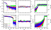 |
Fig. 7. Decay of the galactocentric distance of a tracer particle of mass mt = 10−3M in models with γ = 0 (top left panel) and 1 (bottom left) and the data collapse after a N1/2 scaling (mid panels) to the time-averaged scaling radius, rs, and the evolution of the corresponding mass enclosed with in a sphere of radius 5ϵ centred around mt. The horizontal dotted and dashed lines have the same meaning as in Fig. 3. |
Aiming at comparing with the idealized Chandrasekhar DF, we have also integrated Eq. (14) for mt in the parent smooth models (i.e. setting to 0 the fluctuating term, δf). The dashed black curves in the left panels of Fig. 7 mark the corresponding predicted orbital decay. Notably, in the γ = 0 cored case, the test particle might or might not experience the phase of super-Chandrasekhar DF reported by Read et al. (2006) and Zelnikov & Kuskov (2016), depending on the specific value of N in the simulation at hand. We observe that the onset of the super-Chandrasekhar regime happens at N ≲ 3 × 10⁵, suggesting that it might be connected with low-resolution effects artificially enhancing the collisionality. The same effect is also observable in self-consistent simulations using comparable values of ϵ. Interestingly, for all values of N explored here the test particle stalls at rmt > rs ≳ ϵ. We performed additional tests at fixed N and mt tuning the softening length (and the associated optimal Δt) between 3 × 10⁻⁵rc and 5 × 10⁻²rc, finding that for increasing ϵ, the core stalling sets-in at later times and larger radii. According to the common wisdom, large values of the softening length render an N-body simulation ‘less collisional’ as it depletes the large δf tail of the two-body force distribution by smoothing the pair interactions. At the same time, a large ϵ also hinders the DF by reducing the effective Coulomb logarithm (Marcos et al. 2017; Ma et al. 2023).
Once mt has stalled around rs, the fraction of the host system’s mass that surrounds it (i.e. the mass fraction enclosed in a fixed sphere centred on the instantaneous position of mt) remains almost constant, even in the simulations without self-gravity among the field particles. In the right panels of Fig. 7 we show as a function of time the mass fraction, Md < 5ϵ/M, inside a bona fide radius, d = 5ϵ (roughly of the same order of rinf for mt = 10−3M). For the cored model (top right panel), modulo some resolution-dependent fluctuation, the value of Md < 5ϵ is practically the same for all N, while in the case of a cuspy system (bottom right panel), Md < 5ϵ at core stalling has the same value for N ≳ 105. In other words, since at fixed mt/M one has in our units approximately the same value of rinf (cfr. Eq. (4)), this means that the test particle accretes the same amount of mass5 within its influence radius regardless of the specific resolution given by N. In practice, for increasing N a systematically larger number of orbits is trapped around mt and essentially becomes a ‘dressed particle’, possibly contributing to a more significant erosion of the central density of cuspy systems via stronger field particle ejection (see Fig. 4).
As was expected, at fixed M and N, increasing values of mt (marked by increasingly light shades of blue) result in lower stalling radii, as is shown in the top panel of Fig. 8 for γ = 0, N = 106, and values of the test particle mass in the range of 2 × 10⁻⁴ ≤ mt/M ≤ 10−2. Consistently with the predictions of the Chandrasekhar DF formula (represented in the figure by the dashed lines), heavier particles also sink in a shorter time. The mass enclosed within 5ϵ around their position of mt (bottom panel of Fig. 8) settles in general to slightly lower values for larger mt (i.e. of the order of a 8% difference between the largest and lowest values of the test mass considered here). This might appear in contradiction with what is shown in Figure 7 (right panels) where at fixed mt, Md < 5ϵ is practically independent on N (and thus on mt/m). However, one must notice that larger values of mt at fixed m, associated with lower rs, might scatter the field masses, m, more efficiently, depopulating the control sphere at d = 5ϵ.
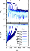 |
Fig. 8. Decay of the galactocentric distance in a γ = 0 cored system for test particles with masses in the range of 2 × 10⁻⁴ ≤ mt/M ≤ 10−2 and N = 106 (top panel) indicated by increasingly light shades of blue. The dashed lines mark the radial decay predicted by the Chandrasekhar formula. Evolution of the mass enclosed with in a sphere of radius 5ϵ centred around mt (bottom panel). |
In Figure 9 we show the relation between the stalling radius and the ratio mt/m for two resolutions, N = 5 × 10⁵ (diamonds) and N = 106 (squares). For both sets of points the trend is rather well described by  , where C is a dimensionless constant of order unity. The stalling radius appears to have the same dependence on m/mt as the wander radius6, rwan, defined in Eq. (3). We interpret this as another indication of the origin of the core stalling as a balance between friction and noise in a central potential, as was originally envisaged for the derivation of rwan with a Fokker-Planck approach (see again Bahcall & Wolf 1976). We note that other studies, such as Read et al. (2006) or Cole et al. (2012), report a general trend of rs ∝ rc/2, even in direct runs with a resolution as large as N = 4 × 10⁶. We conjecture that this apparent discrepancy with our numerical results could be related to their rather large softening length, ranging from ≈rc/3 to 3rc in some runs. We performed additional test runs at fixed N, mt, and γ (not shown here), finding that the stalling radius, rs, is systematically larger for increasing ϵ.
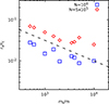 |
Fig. 9. Stalling radius in a γ = 0 model as a function of the mass ratio, mt/m, for the two system resolutions N = 5 × 10⁵ (red diamonds) and N = 106 (blue squares). The dashed line marks the (mt/m)−1/2 trend. |
3.3. Stochastic simulations
Aiming to explore larger values of N not accessible in direct N-body simulations, we have carried out additional numerical experiments evolving the same initial orbits of Fig. 6 using Equation (14) with resolutions up to N = 1013, roughly corresponding to the number of stars in a giant elliptical galaxy. Figure 10 presents rs/rc as function of N for the stochastic simulations with a γ = 0 (circles) and γ = 1 (triangles) parent galaxy model. Remarkably, in the interval of N where we have also performed fully self-consistent N-body and simpler simulations with non-interacting field particles, we recover the same N−1/2 trend (dashed line) with similar values for rs/rc to that reported in Fig. 6. For the cuspy systems, such a trend extends up to N ≈ 109, where for mt = 10−3M the amplitude of the fluctuations, δf, stops balancing a significant fraction of the DF drag, then transitions to a shallower N−1/6, indicated by the dotted brown line. The origin of this slope change remains unclear. We speculate that it could be a numerical artefact related to the choice of Δt in the solution of Eq. (14). In the cored model, the slope change happens at around N ≈ 107, leading to a seemingly N-invariant rs/rc at fixed mt for values of N larger than 109. For larger values of mt, rs systematically decreases for fixed values of N, while the slope changes move at lower N. It must be pointed out that, for values of the test mass larger than ≈M/50, for which in large N models the effect of the force fluctuations would be essentially immaterial, the present linear approximation of the DF fails as mt would typically induce significant perturbations of both the local density and velocity distribution, well before sinking into the core. Unfortunately, checking via N-body the nature of the slope change between N ≈ 107 and 109 is made harder by the fact that the associated value of rs is around ϵ for N ≈ 108, a radius that typically encloses for γ = 1 a rather small number (order unity) of simulation particles, possibly enhancing the amplitude of the discreteness effects while hardly being coherent with the perturbed smooth potential approximation modelled by Eq. (14).
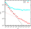 |
Fig. 10. Core-stalling radius as function of N for a particle of mass mt = 10−3M in a cored model (γ = 0, cyan circles) and a mildly cuspy model (γ = 1, red triangles) as extrapolated from Langevin simulations. As in Fig. 6 the dashed lines mark the N1/2 best fit law in the range 104 ≤ N ≤ 3 × 10⁶. |
To illustrate the interplay between the contributions of the different force terms in Equation (14), in Figure 11 we plot for different N the radial dependence of the DF drag force acting on a mass, mt = 10−3M, on a circular orbit with velocity
 (24)
(24)
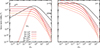 |
Fig. 11. Radial dependence of the DF force acting on a particle of mass mt = 10−3M on a circular orbit at vc (dashed lines), of the typical force fluctuation |

and the typical amplitude of the force fluctuation  , together with the radial gravitational field ||∇Φ(r)||. In the γ = 0 cored model (left panel), the DF term drops significantly for r ≲ 0.1rc as vc tends to 0 while σ is nearly constant, resulting in a vanishing fractional velocity volume function (17). At the same time, for all values of N the typical size of the force fluctuations becomes almost independent on r as
  and α ∝ ρ, with ρ nearly constant below rc for a γ = 0 model. The picture is qualitatively different in the γ = 1 case (right panel), where the decrease in the DF force in the inner regions is way less pronounced and the amplitude of the fluctuating force increases as 1/r2/3. To further clarify how the force fluctuations compete with DF, in Fig. 12 we plot for the same cases of Fig. 11 the difference in the amplitude of fluctuations and the DF force weighted over the local value of the gravitational field, ||∇Φ||. For increasingly large values of N the ratio (α2/3 − ηvc)/||∇Φ|| becomes positive (i.e. force fluctuations mostly balance DF) at smaller radii in units of rc when γ = 1 (right panel). In the γ = 0 systems, for N ≳ 109, the radius at which the change in the trend happens is almost N-independent (left panel), as is evident from Fig. 10, where rs/rc has little to no dependence on N in that resolution range. We noted that such intersections between the curves in Fig. 12 with the horizontal dashed line have the same trend with N as rs/rc in Fig. 10. Remarkably, in the γ = 1 case no apparent slope change at around N ≈ 109 is observed, further indicating a possible numerical origin for that feature. We recall that (see e.g. Gardiner 1994 Chap. 4), the characteristic time, τcr, in which a system described by Eq. (14) relaxes is associated with the inverse of the friction coefficient, η (Spitzer 1969). The latter is essentially the first diffusion coefficient, Df, in the parent Fokker-Planck picture (see Spitzer 1987). The other two coefficients, D⊥ and D∥, associated with perpendicular and parallel heating (i.e. noisy fluctuations of the force) along the trajectory of mt, respectively, are directly proportional to m instead of to mt as for Df. This implies that the timescale on which they effectively operate is typically larger for the cases with smaller values of mt/m, as the dependence on ρ and logΛ is the same as in Df (see the integral expression in Genina et al. 2024). We stress the fact that in the simulation presented here (N-body and stochastic) the integration time is systematically larger or comparable to the inverse of the noise coefficients below rc.
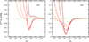 |
Fig. 12. Radial dependence of the difference between the DF term and typical force fluctuation, normalized by the local value of ||∇Φ||, for the same systems shown in Fig. 11. The colour-coding of the curves is the same as in the previous figure. |
4. Outlook and conclusions
Using N-body simulations and stochastic ODE methods, we have investigated the DF acting on a heavy test mass in spherical systems characterized by a cored or cuspy density profile. Previous numerical studies of other authors have often reported a limited or in some cases substantial reduction of the gravitational drag in cored models, with respect to the estimate evaluated by the Chandrasekhar formula (1). Typically, such a discrepancy is interpreted as a consequence of the strong assumptions in the original formulation of DF in infinite and homogeneous systems. More recent semi-analytical work (Banik & van den Bosch 2021, 2022), on the other hand, indicates that DF in cores is naturally suppressed as its coefficient, dominated by the contribution of orbits in resonance with that of the test particle, vanishes towards the centre with the vanishing fraction of nearly resonant particles, in a resolution-independent fashion.
The main results of our work can be summarized as follows. The reduction of the DF force observed in N-body experiments appears to be resolution-dependent (i.e. related to the number of simulation particles when fixing the normalization G = M = rc = 1) in the explored range, 104 ≤ N ≤ 3 × 10⁶, in both cored and cuspy models. The radius at which the test mass, mt, stalls without falling any further to the centre has a marked rcN−1/2 dependence indicative of an underlying Poissonian fluctuation-driven process. Single particle stochastic integrations with an analogous parameter reproduce the same trend, well beyond the N values accessible by the direct simulations (Fig. 10). We observe that approximating the distribution of force fluctuations in said experiments with a Holtsmark function, accommodated to the local values of density and mean particle mass, nicely recovers the behaviour of orbits obtained by N-body simulations. Moreover, the histogram of such force fluctuations, obtained from N-particle realizations of a given system, fits remarkably well the Holtsmark distribution over a large interval of radii. Comparing fully self-consistent runs with others in which the field particles do not interact with one another but propagate as independent tracers in the smooth potential of the model reveals that in the range of 3 × 10⁻⁴ ≲ mt/M ≲ 10−2 the contribution of a self-gravitating wake does not significantly enhance the DF. The stalling radius determined from N-body simulations has a trend that is reasonably compatible,  . This is reminiscent of what was obtained for the wander radius of black holes in dense stellar systems. It must be pointed out that Merritt et al. (2007), in N-body experiments of BHs wandering in γ models, using a simulation set-up essentially analogous to ours, determined that said rwan in cusps broken below the influence radius, rinf, could scale with mt with a much shallower power law. This arises as the BHs’ typical velocity at equilibrium was found to be ⟨v2⟩∝mt−1/(γ − 1), while the rms of its radial position is given by
  when a linear restoring force is present (i.e. inside a nearly flatted out cusp the potential could reasonably be taken as harmonic). Nevertheless, we interpret the similarity of the trend in rs and (the expected one) in rwan as an additional confirmation of the fact that core-stalling induced by a balance between friction and force fluctuations is the same phenomenon at the origin of a mass-dependent wander radius for a heavy particle starting at rest from the centre of the potential well of a star cluster or galactic nucleus.
From the stochastic simulations, we extrapolate that in cuspy models the interplay between friction and fluctuation-related noise balances at smaller radii for increasing N (up to a regime in which δf becomes virtually inexistent), while for cored models there is a critical size (N* ≈ 3 × 10⁷ for mt ≈ 10−3M) above which friction and noise counter each other seemingly independently of the resolution. We must point out that in the continuum limit (i.e. N → ∞; m → 0), in principle, both friction and noise should vanish, leaving mt under the effect of Φ only. At variance with the analogous problems in plasma physics, where typically one deals with N of the order of the Avogadro constant, a stellar system with N ≈ 1012 is still far from being considered a continuum, and is still subjected to a certain degree to a ‘discreteness effect’.
In conclusion, the results of the present work are not in contrast with the resonance-based and N-independent argument of Banik & van den Bosch (2022) that ascribes the core stalling to the vanishing friction coefficient in cores. Indeed, our findings reconcile the predicted N-independent cores stalling with the observed resolution dependent stalling radius, rs, reported by other N-body studies. In other words, for system sizes of the order of N ∼ 103 up to 106, the radial interval over which both the friction and noise terms in Eq. (14) are non-negligible with respect to the local smooth force field is significantly larger, regardless of the fact that the model is cuspy or cored. In cored models, for a sufficiently small test mass, mt, the further outward extent of this interval is larger than the critical radius at which the DF force on a nearly circular orbit begins to drop significantly. For increasing resolution (i.e. larger values of N at fixed normalization and mt/M), in cored models the r-independent fluctuations are smaller and counter DF nearly the same radius below which the friction coefficient has dropped off about two decades over less than a decade in radii (cfr. Figs. 11 and 12). In the end, observing the onset of a resonance-driven core stalling in N-body experiments remains a challenging task, as serial direct numerical simulations are strongly limited in resolution. However, considering a test mass moving in a host system where field particles do not feel their mutual self gravity but orbit in a time-independent field is a problem that can be easily partitioned over different cores or graphic units, allowing for a N up to 1010. In this set-up, choosing a distribution function entirely constituted by circular orbits (that would likely be unstable when accounting for the self consistent forces) could serve as a computational test to probe a possible resonant-driven suppression of the DF.
Models with the same density profile ρ supported by different velocity distribution distributions can exert considerably different friction on the same mass with analogous orbital parameters. In particular, DF in radially anisotropic Osipkov-Merritt models has been found to be less effective than in the associated isotropic system (see Appendix B in Kavanagh et al. 2025).
We note that a substantial mitigation of the DF force on stellar bars (e.g. see Weinberg 1985), ascribed to the suppression of the torque acting on the bar, has also been reported recently by Chiba & Kataria 2024 in systems with DM halos with prograde rotation with respect to the galaxy’s disk.
In general, the model appears to be more sensible to the specific form of ℱ(δf) than that of Ξ(v), see e.g. Pasquato et al. (2018), Pasquato & Di Cintio (2020) for the case in which mt ≈ 2m.
Notably, Agekyan (1962) investigated the distribution of force fluctuations on a test particle surrounded by a finite number,  , of equal field particles, finding a rather good agreement with the Holtsmark distribution.
We verified by checking particles indexes that the particles that ‘dress’ mt are the same ones over the core stalling phase of the dynamics.
Actually, N-body simulations by Merritt et al. (2007) evidenced that the wander radius of a BH embedded in a γ model might depend on its mass, mBH, with a much shallower power law than that of Eq. (3), as the root mean square (rms) of its Brownian velocity scales as  , implying a larger radial excursion even for large BH mass values, with respect to the predictions.
Acknowledgments
We thank Uddipan Banik, Frank van den Bosch, and Carlo Nipoti for the important discussions at different stages of this project. The anonymous Referee is also thanked for his/her valuable comments that helped improving the presentation of our results. This research was supported in part by grant NSF PHY-2309135 to the Kavli Institute for Theoretical Physics (KITP). PFDC wishes to thank the hospitality of the “Laboratoire J.-A. Dieudonné” at the university of Côte d’Azur where part of this work was completed. BM acknowledges support by the grant Segal ANR-19-CE31-0017 of the French Agence Nationale de la Recherche.
References
- Agekyan, T. A. 1962, Soviet Ast., 5, 809 [Google Scholar]
- Ahmad, A., & Cohen, L. 1973, ApJ, 179, 885 [Google Scholar]
- Ahmad, A., & Cohen, L. 1974, ApJ, 188, 469 [Google Scholar]
- Arena, S. E., & Bertin, G. 2007, A&A, 463, 921 [NASA ADS] [CrossRef] [EDP Sciences] [Google Scholar]
- Arena, S. E., Bertin, G., Liseikina, T., & Pegoraro, F. 2006, A&A, 453, 9 [NASA ADS] [CrossRef] [EDP Sciences] [Google Scholar]
- Bahcall, J. N., & Wolf, R. A. 1976, ApJ, 209, 214 [NASA ADS] [CrossRef] [Google Scholar]
- Banik, U., & van den Bosch, F. C. 2021, ApJ, 912, 43 [NASA ADS] [CrossRef] [Google Scholar]
- Banik, U., & van den Bosch, F. C. 2022, ApJ, 926, 215 [NASA ADS] [CrossRef] [Google Scholar]
- Bekenstein, J. D., & Maoz, E. 1992, ApJ, 390, 79 [NASA ADS] [CrossRef] [Google Scholar]
- Bertin, G., Liseikina, T., & Pegoraro 2003, A&A, 405, 73 [NASA ADS] [CrossRef] [EDP Sciences] [Google Scholar]
- Bílek, M., Combes, F., Nagesh, S. T., & Hilker, M. 2024, A&A, 690, A119 [NASA ADS] [CrossRef] [EDP Sciences] [Google Scholar]
- Binney, J., & Tremaine, S. 2008, Galactic Dynamics: Second Edition (Princeton, NJ USA: Princeton University Press) [Google Scholar]
- Bontekoe, T. R., & van Albada, T. S. 1987, MNRAS, 224, 349 [Google Scholar]
- Brockamp, M., Baumgardt, H., & Kroupa, P. 2011, MNRAS, 418, 1308 [CrossRef] [Google Scholar]
- Burrage, K., Lenane, I., & Lythe, G. 2007, SIAM J. Sci. Comput., 29, 245 [Google Scholar]
- Chandrasekhar, S. 1943a, ApJ, 97, 255 [Google Scholar]
- Chandrasekhar, S. 1943b, ApJ, 97, 263 [NASA ADS] [CrossRef] [Google Scholar]
- Chandrasekhar, S. 1943c, ApJ, 98, 54 [NASA ADS] [CrossRef] [Google Scholar]
- Chandrasekhar, S. 1943d, Rev. Mod. Phys., 15, 1 [CrossRef] [Google Scholar]
- Chandrasekhar, S., & von Neumann, J. 1942, ApJ, 95, 489 [NASA ADS] [CrossRef] [Google Scholar]
- Chandrasekhar, S., & von Neumann, J. 1943, ApJ, 97, 1 [NASA ADS] [CrossRef] [Google Scholar]
- Chatterjee, P., Hernquist, L., & Loeb, A. 2002a, Phys. Rev. Lett., 88, 121103 [NASA ADS] [CrossRef] [Google Scholar]
- Chatterjee, P., Hernquist, L., & Loeb, A. 2002b, ApJ, 572, 371 [NASA ADS] [CrossRef] [Google Scholar]
- Chatterjee, P., Hernquist, L., & Loeb, A. 2003, ApJ, 592, 32 [Google Scholar]
- Chiba, R., & Kataria, S. K. 2024, MNRAS, 528, 4115 [Google Scholar]
- Chiron, D., & Marcos, B. 2019, J. Math. Phys., 60, 052901 [Google Scholar]
- Ciotti, L. 2021, Introduction to Stellar Dynamics (Cambridge University Press) [Google Scholar]
- Cole, D. R., Dehnen, W., Read, J. I., & Wilkinson, M. I. 2012, MNRAS, 426, 601 [Google Scholar]
- Dattathri, S., van den Bosch, F. C., Weinberg, M. D., & Banik, U. 2025, arXiv e-prints [arXiv:2505.23905] [Google Scholar]
- Dehnen, W. 1993, MNRAS, 265, 250 [NASA ADS] [CrossRef] [Google Scholar]
- Dehnen, W. 2000, ApJ, 536, L39 [NASA ADS] [CrossRef] [Google Scholar]
- Del Popolo, A. 1996a, A&A, 305, 999 [NASA ADS] [Google Scholar]
- Del Popolo, A. 1996b, A&A, 311, 715 [NASA ADS] [Google Scholar]
- Di Cintio, P., Ciotti, L., & Nipoti, C. 2015, J. Plasma Phys., 81, 495810504 [CrossRef] [Google Scholar]
- Di Cintio, P., Ciotti, L., & Nipoti, C. 2020, in Star Clusters: From the Milky Way to the Early Universe, eds. A. Bragaglia, M. Davies, A. Sills, & E. Vesperini, IAU Symposium, 351, 93 [NASA ADS] [Google Scholar]
- Di Cintio, P., Pasquato, M., Barbieri, L., Trani, A. A., & di Carlo, U. N. 2023, A&A, 673, A8 [NASA ADS] [CrossRef] [EDP Sciences] [Google Scholar]
- Dutta Chowdhury, D., van den Bosch, F. C., & van Dokkum, P. 2019, ApJ, 877, 133 [NASA ADS] [CrossRef] [Google Scholar]
- El-Zant, A. A., Everitt, M. J., & Kassem, S. M. 2019, MNRAS, 484, 1456 [NASA ADS] [CrossRef] [Google Scholar]
- Gabrielli, A., Joyce, M., & Morand, J. 2014, Phys. Rev. E, 90, 062910 [Google Scholar]
- Gardiner, C. W. 1994, Handbook of stochastic methods for physics, chemistry and the natural sciences (Berlin: Springer) [Google Scholar]
- Genina, A., Springel, V., & Rantala, A. 2024, MNRAS, 534, 957 [CrossRef] [Google Scholar]
- Gilbert, I. H. 1970, ApJ, 159, 239 [Google Scholar]
- Goerdt, T., Moore, B., Read, J. I., Stadel, J., & Zemp, M. 2006, MNRAS, 368, 1073 [Google Scholar]
- Goerdt, T., Moore, B., Read, J. I., & Stadel, J. 2010, ApJ, 725, 1707 [Google Scholar]
- Hamilton, C., Fouvry, J.-B., Binney, J., & Pichon, C. 2018, MNRAS, 481, 2041 [NASA ADS] [CrossRef] [Google Scholar]
- Hernquist, L. 1990, ApJ, 356, 359 [Google Scholar]
- Heyvaerts, J., Fouvry, J.-B., Chavanis, P.-H., & Pichon, C. 2017, MNRAS, 469, 4193 [NASA ADS] [CrossRef] [Google Scholar]
- Holtsmark, J. 1919, Ann. Phys., 363, 577 [CrossRef] [Google Scholar]
- Huang, S., Dubinski, J., & Carlberg, R. G. 1993, ApJ, 404, 73 [Google Scholar]
- Inoue, S. 2011, MNRAS, 416, 1181 [NASA ADS] [CrossRef] [Google Scholar]
- Kalnajs, A. J. 1972, in IAU Colloq. 10: Gravitational N-Body Problem, ed. M. Lecar, Astrophysics and Space Science Library, 31, 13 [Google Scholar]
- Kandrup, H. E. 1980, Phys. Rep., 63, 1 [NASA ADS] [CrossRef] [Google Scholar]
- Kandrup, H. E. 1983, Ap&SS, 97, 435 [NASA ADS] [CrossRef] [Google Scholar]
- Kaur, K., & Sridhar, S. 2018, ApJ, 868, 134 [Google Scholar]
- Kaur, K., & Stone, N. C. 2022, MNRAS, 515, 407 [Google Scholar]
- Kavanagh, B. J., Karydas, T. K., Bertone, G., Di Cintio, P., & Pasquato, M. 2025, Phys. Rev. D, 111, 063071 [Google Scholar]
- Kazantzidis, S., Magorrian, J., & Moore, B. 2004, ApJ, 601, 37 [NASA ADS] [CrossRef] [Google Scholar]
- Londrillo, P., Nipoti, C., & Ciotti, L. 2003, Mem. Soc. Astron. Ital. Suppl., 1, 18 [Google Scholar]
- Lynden-Bell, D., & Kalnajs, A. J. 1972, MNRAS, 157, 1 [Google Scholar]
- Ma, L., Hopkins, P. F., Kelley, L. Z., & Faucher-Giguère, C.-A. 2023, MNRAS, 519, 5543 [NASA ADS] [CrossRef] [Google Scholar]
- Mannella, R. 2004, Phys. Rev. E, 69, 041107 [NASA ADS] [CrossRef] [Google Scholar]
- Maoz, E. 1993, MNRAS, 263, 75 [NASA ADS] [Google Scholar]
- Marcos, B., Gabrielli, A., & Joyce, M. 2017, Phys. Rev. E, 96, 032102 [NASA ADS] [CrossRef] [Google Scholar]
- Marochnik, L. S. 1968, Soviet Ast., 11, 873 [Google Scholar]
- Merritt, D., Berczik, P., & Laun, F. 2007, AJ, 133, 553 [NASA ADS] [CrossRef] [Google Scholar]
- Mikkola, S., & Merritt, D. 2006, MNRAS, 372, 219 [NASA ADS] [CrossRef] [Google Scholar]
- Miocchi, P., Pasquato, M., Lanzoni, B., et al. 2015, ApJ, 799, 44 [NASA ADS] [CrossRef] [Google Scholar]
- Mulder, W. A. 1983, A&A, 117, 9 [NASA ADS] [Google Scholar]
- Nasim, I. T., Gualandris, A., Read, J. I., et al. 2021, MNRAS, 502, 4794 [NASA ADS] [CrossRef] [Google Scholar]
- Nipoti, C., Londrillo, P., & Ciotti, L. 2006, MNRAS, 370, 681 [NASA ADS] [CrossRef] [Google Scholar]
- Pasquato, M., & Di Cintio, P. 2020, A&A, 640, A79 [NASA ADS] [CrossRef] [EDP Sciences] [Google Scholar]
- Pasquato, M., Miocchi, P., & Yoon, S.-J. 2018, ApJ, 867, 163 [NASA ADS] [CrossRef] [Google Scholar]
- Peebles, P. J. E. 1972, ApJ, 178, 371 [NASA ADS] [CrossRef] [Google Scholar]
- Petrovskaya, I. V. 1986, Soviet. Astron. Lett., 12, 237 [Google Scholar]
- Petts, J. A., Gualandris, A., & Read, J. I. 2015, MNRAS, 454, 3778 [NASA ADS] [CrossRef] [Google Scholar]
- Petts, J. A., Read, J. I., & Gualandris, A. 2016, MNRAS, 463, 858 [NASA ADS] [CrossRef] [Google Scholar]
- Plummer, H. C. 1911, MNRAS, 71, 460 [Google Scholar]
- Pogorelov, I. V., & Kandrup, H. E. 1999, Phys. Rev. E, 60, 1567 [Google Scholar]
- Read, J. I., Goerdt, T., Moore, B., et al. 2006, MNRAS, 373, 1451 [NASA ADS] [CrossRef] [Google Scholar]
- Sartorello, S., Di Cintio, P., Trani, A. A., & Pasquato, M. 2025, A&A, 698, A28 [NASA ADS] [CrossRef] [EDP Sciences] [Google Scholar]
- Spitzer, L., Jr 1969, ApJ, 158, L139 [NASA ADS] [CrossRef] [Google Scholar]
- Spitzer, L. 1987, Dynamical evolution of globular clusters (Princeton, N.J.: Princeton University Press) [Google Scholar]
- Terzic, B., & Kandrup, H. E. 2003, arXiv e-prints [arXiv:astro-ph/0312434] [Google Scholar]
- Trani, A. A., & Di Cintio, P. 2025, arXiv e-prints [arXiv:2506.02173] [Google Scholar]
- Tremaine, S., & Weinberg, M. D. 1984, MNRAS, 209, 729 [Google Scholar]
- Tremaine, S., Richstone, D. O., Byun, Y.-I., et al. 1994, AJ, 107, 634 [CrossRef] [Google Scholar]
- van Albada, T. S., & Szomoru, A. 2020, in Star Clusters: From the Milky Way to the Early Universe, eds. A. Bragaglia, M. Davies, A. Sills, & E. Vesperini, IAU Symposium, 351, 532 [Google Scholar]
- Weinberg, M. D. 1985, MNRAS, 213, 451 [Google Scholar]
- White, S. D. M. 1983, ApJ, 274, 53 [Google Scholar]
- Zelnikov, M. I., & Kuskov, D. S. 2016, MNRAS, 455, 3597 [NASA ADS] [CrossRef] [Google Scholar]
Appendix A: Analytical dynamical friction coefficient for the Plummer sphere
The DF expressed in Eq. (1) is often evaluated assuming that the phase space distribution of the underlying model can be factorized as f(r, v) = ρ(r)f(v). In the commonly adopted local Maxwellian approximation, the position dependence of the velocity distribution f(v) is restored by assuming a Maxwellian distribution with velocity dispersion proportional to r via the Jeans equations for the associated density potential pair (ρ, Φ). In principle, in a spherically symmetric model with isotropic phase space distribution, the integral in Eq. (2) could be instead carried out over f(ℰ) = f(r, v). However, most often f has a rather complicated form even for simple density profiles such as the γ-models. For the Plummer distribution, where f(ℰ) is given by Eq. (12) the integration becomes rather easy (e.g. see Miocchi et al. 2015) and one has
 (A.1)
(A.1)
In the equation above  ,
,  and
and  . Setting
  one has
![Mathematical equation: $$ \begin{aligned} \Xi ^*(r,v)=\alpha \Psi ^5\bigg [\frac{1}{2}\tan ^{-1}(u)+\bigg (\frac{u^9}{2}-\frac{79}{21}u^7-\frac{64}{15}u^5-\frac{7}{3}u^3-\frac{u}{2}\bigg )\nonumber \\ \times (1+u^2)^{-5}-\frac{\pi }{4}\bigg ], \end{aligned} $$](/articles/aa/full_html/2025/08/aa55427-25/aa55427-25-eq46.gif) (A.2)
(A.2)
where  .
.
In Fig. A.1 we show the radial profile of the DF force acting on a test mass mt = 10−3M moving on a circular orbit at the local circular velocity  , evaluated in the local Maxwellian approximation (dashed lines) and integrating over the distribution function (solid line), so that the term ρΞ(v) in Equation (1) is substituted by Ξ*(r, v) defined above. At r ≫ rc the two expressions do not give appreciably different drag force, while below r ≈ 5 × 10⁻¹rc, the local Maxwellian approximation overestimates the DF of a factor about 1.4, we conclude that using such approximate form for the friction force does not alter significantly its effect, in particular since the region where the error is greater corresponds to a radial range where its contribution itself becomes under-dominant.
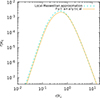 |
Fig. A.1. Radial profile of the DF force on a mass mt = 10−3M on a circular orbit in a Plummer model. |
Appendix B: Further comparison between self-consistent and tracer simulations
As the asymptotic stalling radius is roughly the same in self-consistent simulation and simplified smooth potential and tracer ones, we expect that the (relative) energy of mt relaxes to comparable values once the its radial coordinate has settled at ≈rs. In Fig. B.1 we show the evolution of ℰ for the same runs of Fig. 3. In this case, where the resolution is N = 106 we observe a remarkably good agreement of the final values of the relative energy for both values of γ with relatively small fluctuations. Smaller values of N (not shown here) also yield rather similar values, though bearing larger fluctuations around the final value for N ≲ 105. By contrast, the norm of the angular momentum J shown for the same simulations in Fig. B.2 shows wilder fluctuations (even at N as large as 3 × 10⁶), of about the 10% of its asymptotic value. We interpret this as a result of the more chaotic behaviour of orbits in the inner region of both models that reflects in violent changes in orbital eccentricity and inclination while the energy remains nearly constant.
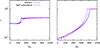 |
Fig. B.1. Evolution of the relative orbital energy per unit mass ℰ for a test mass mt = 10−3 in a γ = 0 (left) and γ = 1 (right) model. In both cases N = 106 and the blue and magenta curves refer to the tracer in smooth potential and self-consistent runs, respectively. |
All Figures
|
Fig. 1. Radial profile of the average of the discrete force fluctuations (left panel) and its variance (right panel) evaluated for a single realization of a Plummer system with N = 106. |
| In the text | |
|
Fig. 2. Numerically evaluated distribution of force fluctuation, 𝒫(δf), in different shells of increasing radius (clockwise from top left, r = 3.1 × 10⁻², 7.2 × 10⁻², 0.38, 1.3, 6.9, and 54.8 in units of rc) for a Plummer model with N = 106 and 102 realizations (grey dots). The blue dots mark the PDF averaged over said ensemble, while the red curve is the corresponding the Holtsmark distribution (15) computed for the local value of the density, ρ(r), and average number of particles in the shell, |
| In the text | |
|
Fig. 3. Radial decay of a massive tracer, mt = 10−3M, orbiting in a γ = 0 (left) and a γ = 1 (right) model in a self consistent N-body run (blue curves) and a simplified simulation where the same N = 106 field particles move independently in the static smooth potential (magenta curves). The horizontal dashed orange line marks the value of the softening parameter ϵ = 2 × 10⁻³rc, while the dotted black line indicates the radius, rmt, at which M(r) = mt, equal to ≈0.1 for the simulations with γ = 0 and ≈0.033 for those with γ = 1. |
| In the text | |
|
Fig. 4. Initial density profile corresponding to a γ = 0 (top) and a γ = 1 (bottom) model (filled orange squares) and corresponding density profiles at t = 103tc in the self-consistent and tracers in smooth potential simulations (upward blue triangles and downward magenta triangles, respectively). The dashed black lines mark ρ(r) as given in Eq. (5). The points correspond to the same simulations of Fig. 3. |
| In the text | |
|
Fig. 5. Decay of the galactocentric distance in a Plummer system for a particle with mt = 2 × 10⁻³M in a N-body simulation with N = 106 (magenta curve), and two semi-analytical integrations in the parent smooth potential with DF and fluctuations (solid cyan line) and with DF only (dashed black line). |
| In the text | |
|
Fig. 6. Core-stalling radius as function of N for a particle of mass mt = 10−3M in a cored model (γ = 0, circles) and a mildly cuspy model (γ = 1, triangles). Filled magenta symbols refer to the full self-consistent N-body simulations, and empty blue ones to the simulations with non-interacting tracers. To guide the eye, the dashed line marks the N−1/2 trend. |
| In the text | |
|
Fig. 7. Decay of the galactocentric distance of a tracer particle of mass mt = 10−3M in models with γ = 0 (top left panel) and 1 (bottom left) and the data collapse after a N1/2 scaling (mid panels) to the time-averaged scaling radius, rs, and the evolution of the corresponding mass enclosed with in a sphere of radius 5ϵ centred around mt. The horizontal dotted and dashed lines have the same meaning as in Fig. 3. |
| In the text | |
|
Fig. 8. Decay of the galactocentric distance in a γ = 0 cored system for test particles with masses in the range of 2 × 10⁻⁴ ≤ mt/M ≤ 10−2 and N = 106 (top panel) indicated by increasingly light shades of blue. The dashed lines mark the radial decay predicted by the Chandrasekhar formula. Evolution of the mass enclosed with in a sphere of radius 5ϵ centred around mt (bottom panel). |
| In the text | |
|
Fig. 9. Stalling radius in a γ = 0 model as a function of the mass ratio, mt/m, for the two system resolutions N = 5 × 10⁵ (red diamonds) and N = 106 (blue squares). The dashed line marks the (mt/m)−1/2 trend. |
| In the text | |
|
Fig. 10. Core-stalling radius as function of N for a particle of mass mt = 10−3M in a cored model (γ = 0, cyan circles) and a mildly cuspy model (γ = 1, red triangles) as extrapolated from Langevin simulations. As in Fig. 6 the dashed lines mark the N1/2 best fit law in the range 104 ≤ N ≤ 3 × 10⁶. |
| In the text | |
|
Fig. 11. Radial dependence of the DF force acting on a particle of mass mt = 10−3M on a circular orbit at vc (dashed lines), of the typical force fluctuation |
| In the text | |
|
Fig. 12. Radial dependence of the difference between the DF term and typical force fluctuation, normalized by the local value of ||∇Φ||, for the same systems shown in Fig. 11. The colour-coding of the curves is the same as in the previous figure. |
| In the text | |
|
Fig. A.1. Radial profile of the DF force on a mass mt = 10−3M on a circular orbit in a Plummer model. |
| In the text | |
|
Fig. B.1. Evolution of the relative orbital energy per unit mass ℰ for a test mass mt = 10−3 in a γ = 0 (left) and γ = 1 (right) model. In both cases N = 106 and the blue and magenta curves refer to the tracer in smooth potential and self-consistent runs, respectively. |
| In the text | |
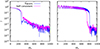 |
Fig. B.2. Evolution of the norm of the orbital angular momentum J for the same systems of Fig. B.1. |
| In the text | |
Current usage metrics show cumulative count of Article Views (full-text article views including HTML views, PDF and ePub downloads, according to the available data) and Abstracts Views on Vision4Press platform.
Data correspond to usage on the plateform after 2015. The current usage metrics is available 48-96 hours after online publication and is updated daily on week days.
Initial download of the metrics may take a while.