| Issue |
A&A
Volume 700, August 2025
|
|
|---|---|---|
| Article Number | A254 | |
| Number of page(s) | 11 | |
| Section | Interstellar and circumstellar matter | |
| DOI | https://doi.org/10.1051/0004-6361/202555597 | |
| Published online | 25 August 2025 | |
Measuring the initial mass of 44Ti in SN 1987A through the 44Sc emission line
1
Dipartimento di Fisica e Chimica E. Segrè, Università degli Studi di Palermo,
Via Archirafi 36,
90123
Palermo,
Italy
2
INAF-Osservatorio Astronomico di Palermo,
Piazza del Parlamento 1,
90134
Palermo,
Italy
3
AIM, CEA, CNRS, Université Paris-Saclay, Université de Paris,
91191
Gif sur Yvette,
France
4
Institute of Astronomy and Astrophysics, Academia Sinica,
Taipei
106319,
Taiwan
5
Astrophysical Big Bang Laboratory (ABBL), RIKEN Cluster for Pioneering Research,
2-1 Hirosawa, Wako,
Saitama
351-0198,
Japan
6
Institute for Applied Problems in Mechanics and Mathematics,
Naukova Street 3-b,
79060
Lviv,
Ukraine
7
INAF – Osservatorio Astrofisico di Arcetri,
Largo E. Fermi 5,
50125
Firenze,
Italy
8
RIKEN Center for Interdisciplinary Theoretical and Mathematical Sciences (iTHEMS),
2-1 Hirosawa, Wako,
Saitama
351-0198,
Japan
9
Astrophysical Big Bang Laboratory (ABBL), RIKEN Pioneering Research Institute (PRI),
2-1 Hirosawa, Wako,
Saitama
351-0198,
Japan
10
Astrophysical Big Bang Group (ABBG), Okinawa Institute of Science and Technology Graduate University (OIST),
1919-1 Tancha, Onna-son, Kunigami-gun,
Okinawa
904-0495,
Japan
★ Corresponding author.
Received:
20
May
2025
Accepted:
7
July
2025
Abstract
Context. Deriving the mass and large-scale asymmetries of radioactive isotopes offers valuable insights into the complex phases of a supernova explosion. Important examples include 56Ni, with its decay products 56Co and 56Fe, and 44Ti, which are studied through their X-ray emission lines, and provide a powerful diagnostic tool to probe the explosive nucleosynthesis processes in the inner layers of the exploding star.
Aims. In this framework, SN 1987A provides a privileged laboratory, being the youngest supernova remnant from which the mass of Ti has been estimated. However, some uncertainty remains in determining the initial mass of 44Ti. Previous analyses, relying on NuSTAR and INTEGRAL data, report M44 = (1.5 ± 0.3) × 10−4 M⊙ and M44 = (3.1 ± 0.8) × 10−4M⊙, respectively. In this paper, we estimate the initial mass of 44Ti via its decay product, the 44Sc emission line at 4.09 keV, using Chandra observations.
Methods. We performed multi-epoch spectral analysis focusing on the inner part of the remnant, to minimize the contamination from the X-ray emission stemming from the shocked plasma. As a result, we report the detection of 44Sc emission line in the central part of SN 1987A with a ~99.7% (3 σ) significance.
Results. The simultaneous fit of the spectra extracted from observations between 2016 and 2021 yields a line flux of 6.8−2.3+2.2 × 10⁻⁷ photons s−1 cm−2, corresponding to a 44Ti mass of M44 = (1.6 ± 0.5) × 10−4M⊙ (errors at the 90% confidence level). The results obtained with our spectral analysis appear to align with those derived with NuSTAR.
Key words: supernovae: general / ISM: general / supernovae: individual: SN 1987A
© The Authors 2025
 Open Access article, published by EDP Sciences, under the terms of the Creative Commons Attribution License (https://creativecommons.org/licenses/by/4.0), which permits unrestricted use, distribution, and reproduction in any medium, provided the original work is properly cited.
This article is published in open access under the Subscribe to Open model. This email address is being protected from spambots. You need JavaScript enabled to view it. to support open access publication.
1 Introduction
Supernova (SN) explosions are important sources for studying the chemical evolution of the Universe. The supernova ejecta carry information on explosive nucleosynthesis processes, and elements synthesized in the inner layers of core-collapse supernovae can “retain memory” of the physical mechanisms governing the explosion. Several key issues can be addressed by studying the radioactive emission of the 56Ni and 44Ti isotopes, which are synthesized in the central part of the exploding star (Hashimoto 1995; Nagataki et al. 1997; Nagataki 2000), along with their daughter products, such as 56Co and 56Fe for 56Ni, and 44Sc for 44Ti. In particular, the yield of 44Ti is very sensitive to supernova shock conditions (more so than 56Ni), specifically the peak temperature and density of the ejecta reached shortly after core collapse (e.g., Magkotsios et al. 2010), thus providing a powerful diagnostic tool for explosion physics. Moreover, as shown by Nagataki et al. 1997, 1998 and Nagataki (2000), a high 44Ti/56Ni ratio can be considered a signature of large-scale anisotropies in the explosions. More recently it has been found that neutrino-driven winds and the possible simultaneous accretion and explosion in 3D models of CCSNe are crucial for 44Ti production (Wang & Burrows 2024).
After the complete decay of 56Co and 57Co, which dominate the energy balance during the first few years following the explosion, the IR, optical, and UV emissions are driven by the radioactive decay of 44Ti. Additional evidence for the presence of 44Ti can be derived from the X-ray and γ-ray emission of its decay chain. In this process, 44Ti decays into 44Sc with an e-folding time of 85 years (Ahmad et al. 2006), producing two emission lines at 67.9 keV and 78.4 keV through electron capture. Subsequently, 44Sc decays into 44Ca with a lifetime of 5.7 hours (Ahmad et al. 2006), emitting a line at 1157.0 keV through β-decay and electron capture. The electron capture results in 44Sc with a vacancy in its K-shell, which produces a K-shell transition with an X-ray emission line at 4.09 keV.
The supernova SN 1987A, observed on February 23, 1987 in the Large Magellanic Cloud (West 1987) at a distance d = 51.4 kpc (Panagia 1999), is an ideal target for studying a nearby, very young, core-collapse supernova explosion (CCSN), and its subsequent evolution into a supernova remnant (SNR). X-ray emission from SN 1987A was detected by Dotani et al. (1987) in the hard band (above 10 keV) a few months after the explosion and a few years later by Beuermann et al. (1994) with ROSAT in the soft X-rays. Since 1999, multi-epoch Chandra observations have revealed the morphology of the X-ray emission and its time evolution (Helder et al. 2013; Frank et al. 2016; Ravi et al. 2024; see also Fig. 1). The X-ray emission of SN 1987A is characterized by a ring-like structure in expansion, which results from the shocked circumstellar medium produced by stellar winds from the progenitor star before the SN explosion. The circumstellar medium has been previously observed in the optical band (Luo & McCray 1991; Lundqvist & Fransson 1991; Burrows et al. 1995; Chevalier & Dwarkadas 1995). Important information on the origin and evolution of the X-ray spectral features has been obtained from the analysis of XMM-Newton observations (Haberl et al. 2006; Sun et al. 2021) and SRG/eRosita (Maitra et al. 2022).
The X-ray emission can be well reproduced by magnetohydrodynamic (MHD) simulations (Orlando et al. 2015, 2019, 2020, 2025), which self-consistently describe the time evolution of the remnant morphology, fluxes, and spectra. Moreover, the comparison between X-ray data and MHD simulations provides important information on the origin of the broadening of X-ray emission lines, pinpointing the roles of thermal broadening and Doppler broadening associated with plasma expansion (Miceli et al. 2019; Ravi et al. 2021; Miceli 2023). Recently, XRISM collaboration (2025) have shown that XRISM observations can recover the expansion velocity of the outer (i.e., metal-poor) ejecta layers interacting with the reverse shock, as predicted by Sapienza et al. (2024a,b). Thermal X-ray emission from metal-rich ejecta is expected to be modest in the next few years (Orlando et al. 2025).
Multiwavelength observations of SN 1987A have revealed Doppler shifts in the emission lines of heavy elements (e.g., [Fe II] and [Ni II]) up to velocities exceeding 3000 km s−1 (e.g., Haas et al. 1990; Colgan et al. 1994; Utrobin et al. 1995; Larsson et al. 2016). The formation of 56Co gamma-ray lines in SN 1987A, several months earlier than expected (Matz et al. 1988), reveals mixing between some innermost heavy nuclear products and the outer envelope. The 56Co lines at 847 and 1238 keV were detected by balloon experiments (Cook et al. 1988; Mahoney et al. 1988; Sandie et al. 1988; Teegarden et al. 1989) and by the γ-ray spectrometer (GRS) on board the Solar Maximum Mission (SMM) satellite (Matz et al. 1988; Leising & Share 1990). As a result, it was found that almost 5% of irongroup-rich plasma mixed out to velocities of ~3000 km s−1 (Arnett et al. 1989; Leising & Share 1990), much higher than the characteristic values (≲ 1000 km s−1) expected for iron-group material. This mixing may result from Rayleigh–Taylor instabilities or from radioactive heating, which causes the expansion of 56Ni/56Co-rich bubbles (Basko 1994; Kifonidis et al. 2003; Urushibata et al. 2018; Ono et al. 2020).
The anisotropy in the inner ejecta velocities has been confirmed by the detection of a redshift of approximately 0.23 keV in the 44Ti X-ray emission lines at 67.87 keV (Boggs et al. 2015), observed with NuSTAR and corresponding to a velocity of ~700 km s−1 in the rest frame of SN 1987A. Boggs et al. (2015) measured the flux of the line at 67.87 keV (F68 = 3.5 ± 0.7 × 10⁻⁶ cm−2 s−1; similar results were later obtained by Alp et al. 2021), thus deriving an initial mass of 44Ti M44 = 1.5 ± 0.3 × 10⁻⁴M⊙ (see Eq. (1)). This value is in agreement with the simulations (Thielemann et al. 1990; Woosley & Hoffman 1991), which predict M44 = 0.2-2.5 × 10⁻⁴M⊙ in CCSNe. Modeling of the optical spectrum performed by Jerkstrand et al. (2011) also suggests M44 = 1.5 ± 0.5 × 10⁻⁴M⊙. Furthermore, model B18.3 developed by Orlando et al. (2020) and Ono et al. (2020) predicted an initial 44Ti mass of approximately 1.4 × 10⁻⁴ M⊙. However, this value should be interpreted with caution, as the explosive nucleosynthesis was modeled using a small approximate nuclear reaction network and this may lead to an overestimation of the 44Ti abundance (Mao et al. 2015).
Conversely, the fluxes of the 67.87 keV and 78.32 keV lines measured with INTEGRAL indicate a higher initial 44Ti mass, by a factor of ~2, i.e., M44 = (3.1 ± 0.8) × 10−4 M⊙ (Grebenev et al. 2012).
The 44Ti yield can also be estimated by measuring the flux of the 44Sc line at 4.09 keV, as successfully demonstrated for the supernova remnant G1.9+0.3 by Borkowski et al. (2010), through the analysis of Chandra observations. This approach was also applied to SN 1987A by Leising (2006), who analyzed multi-epoch Chandra spectra of the entire remnant, finding no significant detection of the 44 Sc line due to high contamination by the emission of the shocked ring material. Their upper limit on the line flux corresponds to M44 < 2 × 10⁻⁴ M⊙, without including the effects of photoelectric absorption from the surrounding cold ejecta.
In this paper, we adopt a new methodology to detect the 44Sc line in multi-epoch Chandra observations of SN 1987A and to estimate the value of M44. In particular, we selected a circular region in the inner part of the remnant (with an angular radius R ~ 0.3"; see Fig. 1), where the contamination from thermal emission from the shocked plasma is as low as possible. Additionally, the expansion of the bright ring reduces contamination from thermal emission from shocked plasma in the central region, where 44 Sc is thought to be synthesized, at the latest epochs. We also note that the lowest absorption from the cold ejecta at the latest epochs favors the detection of the 44Sc emission line.
The paper is organized as follows. Sect. 2 describes the observations analyzed and the data reduction. Results are presented in Sects. 3 and 4 and the discussion and conclusions are provided in Sect. 5. Details of the observations are listed in Appendix A. Appendix B shows the temporal evolution of the 44Sc line. The background region and spectrum are presented in Appendix C, while Appendix D shows the complete view of the Markov Chain Monte Carlo (MCMC) corner plot discussed in Sect. 3.
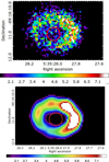 |
Fig. 1 Upper panel: Chandra/ ACIS photon count map of SN 1987A in 2019 (Obs ID 21304), in the 0.5–7.0 keV energy band. Lower panel: same image as above, but deconvolved using the Lucy-Richardson algorithm. Both images have a pixel size of 0.06″. The red circle indicates the region selected for spectral analysis. |
2 Observations and data reduction
We analyzed all archival Chandra/ACIS-S observations of SN 1987A, spanning 22 years from 2000 to 2021. The relevant information on the observations is summarized in Table A.1. Data were analyzed with CIAO (v4.13), using CALDB (v4.9.4), and reprocessed with the chandra_repro task.
For the image analysis, we adopted subpixel sampling with a pixel size of 0.06 arcsec for each observation. We improved the spatial resolution of all images using the CIAO arestore tool, which accounts for the point spread function (PSF) of the telescope by applying the Lucy-Richardson deconvolution algorithm (as previously demonstrated in Helder et al. 2013; Frank et al. 2016; Ravi et al. 2024). To produce the PSF for the deconvolution, we used the MARX software (Davis et al. 2012). The deconvolved image provides a better constraint on the emission from the ring, serving as a good starting point for selecting the region used in the spectral analysis.
Spectra were extracted from the event files using specextract, which also generates the corresponding ancillary response file (ARF) and the redistribution matrix file (RMF). The spectra were rebinned using the optimal binning algorithm of (Kaastra & Bleeker 2016). Spectra extracted from observations performed within one month were merged using the CIAO tool combine_spectra.
Spectra were analyzed using the XSPEC V 12.13.0c soft-ware(Arnaud 1996), in the 1.0–5.5 keV band. Due to the low statistics, we fit the spectra using the C-statistic (Cash 1979). To calculate the error bars, we ran the Markov Chain Monte Carlo (MCMC) algorithm within xspec, thereby accounting for the dependencies among the free parameters in the fit. We used the Goodman-Weare algorithm with a chain length of 2 × 10⁵ and 30 walkers.
3 Results
The isotope 44Ti is synthesized in the innermost ejecta, and its X-ray emission becomes detectable only when the gas is optically thin, i.e., approximately 20 years after the SN explosion (e.g., Fransson & Chevalier 1987). Once the ejecta become transparent to X-rays, the flux corresponding to each radioactive emission line, Fi, can be calculated as
 (1)
(1)
where M44 is the initial mass of 44Ti, d is the distance to the source, mp is the proton mass, t44 is the e-folding time decay of 44Ti (~85 yr), and Wi is the emission efficiency for the three X-ray emission lines (17.4% for line at 4.1 keV, 87.7% for line at 67.87 keV, and 94.7% for line at 78.4 keV, Grebenev et al. 2012).
We expect 44Ti in SN 1987A to be distributed over an extended area, similar to that of Fe-rich ejecta. Larsson et al. (2023) showed that the Fe-rich ejecta are located within the main shell of reverse-shocked material, in a region referred to as the homunculus, well inside the shocked, dense equatorial ring (ER). Accordingly, we selected a circular region with radius 0.3" (shown as a red circle in Fig. 1) for spectral extraction. Within this region, maximum 44Sc line emission is expected from the unshocked ejecta, while, the choice of extraction region simultaneously minimizes the contamination associated with the thermal X-ray emission from the ER.
The source spectrum was fitted with a model that includes interstellar absorption (the Tbabs model) with a column density, NH, fixed at 2.35 × 1021 cm−2 (Park et al. 2006); a nonequilibrium of ionization collisional plasma model (thevnei model), to reproduce thermal emission from the shocked plasma spilling from the bright ring inside the central region because of the telescope PSF; an absorbed power law (with absorption originating from cold ejecta) to account for the nonthermal emission stemming from the putative pulsar wind nebula (Greco et al. 2021, 2022) (the vphabs*pow model); and a Gaussian component for the 44Sc line. The 44Sc line emission is expected to be redshifted as that of 44Ti ((∆E/E)44Ti = (∆E/E)44Sc). Since the emission line at 67.87 keV shows (∆E)44Ti = 0.23 ± 0.09 (Boggs et al. 2015), we expect (∆E)44Sc = 0.013 ± 0.005 keV, yielding the line centered at about 4.076 keV. We kept the line centroid frozen to this value during the fitting process. The model for the source spectra is described by the following equation:
 (2)
(2)
In the early Chandra observations, we expect the absorption from cold ejecta to be prominent at the energy of the 44Sc emission line and the measurement of the line flux to be affected by this issue. A careful search for line emission at 4.076 keV yields very low line fluxes for the observations performed between 2000 and 2015, as described in detail in Appendix B. The detailed modeling of the time-dependent absorption from cold ejecta is beyond the scope of this paper. Given the uncertainties in the distribution of 44Ti in our simulations of SN 1987A (see Ono et al. 2020), it is not possible to perform an accurate estimate of the emission and absorption of the line in the ejecta. However, we caution that this limitation may affect our estimates. We focus here on the spectral analysis of the most recent six years of our set of observations (2016–2021), when the expansion of the remnant significantly reduces thermal contamination in the central region, and the cold ejecta are expected to be optically thin, thereby allowing Eq. (1) to be applied.
To improve the statistics of the 44Sc emission line, we simultaneously fit spectra extracted from all observations performed between 2016 and 2021. When fitting the spectra, the electron temperature, ionization parameter, and normalization of the vnei component of each spectrum were left free to vary. The normalization of the Gaussian component that models the 44Sc line was also a free parameter, but, in this case, the normalizations of different epochs were tied together to account for the expected exponential time decay of Eq. (1). The sigma of the Gaussian component was fixed to 1 × 10⁻³ keV to reduce the number of free parameters. We verified that the results of the fits were not affected when this parameter was left free to vary.
The background region was selected on the same chip as the source region, in an area without visible point-like sources, and the corresponding spectrum was fitted with an ad hoc model (see Appendix C for details). The background flux is consistently less than 0.1% of the total, which is why the background components are not visible in the spectral plots. The data, corresponding best-fit model, and residuals are shown in the upper panel of Fig. 2.
The angular extension of the spectral extraction region shown in Fig. 1 (0.3") is smaller than the Chandra PSF (~0.5"), so that a fraction of the photons emitted within the central region are scattered outside it by the telescope mirrors. Larsson et al. (2023) showed that the unshocked Fe-rich ejecta in SN 1987A extend over a large area inside the ER, largely filling the spectral extraction region. As a working assumption, we assume that the Ti-rich ejecta are uniformly distributed within the extraction region (Ono et al. 2020). Under this hypothesis, the 44Sc line emission originates from a disk with radius 0.3″. Using the MARX software, we find that, in this scenario, three-quarters of the photons are scattered outside the region. A very similar proportion (71%) is obtained by assuming a 2D Gaussian profile with σ = 0.15″. Although this percentage may vary slightly depending on different spatial distributions of surface brightness within the extraction region, we expect that the line flux obtained from the spectral analysis needs to be multiplied by a factor f of the order of f ≈ 4 to recover its intrinsic value. We adopt f = 4 hereafter.
From the combined analysis of the 2016–2021 spectra, we find a line flux of  photons s−1 cm−2, with error bars at the 90% confidence level. For visualization purposes, the lower panel of Fig. 2 shows the combined Chandra/ACIS spectrum obtained by summing all spectra collected between 2016 and 2021. The 44Sc line is clearly visible above the continuum. Fig. 3 shows a portion of the MCMC corner plot for the first four free parameters: the normalization of the Gaussian centered at 4.076, the electron temperature kT, the ionization age τ, and the normalization of the first vnei component associated with the spectrum observed in 2016. Contours correspond to the 68%, 95.5%, and 99.7% confidence levels. The corresponding complete corner plot is shown in Fig. D.1 and indicates a detection significance of approximately 3σ (99.7% confidence level). We conclude that the detection of the line is robust and statistically significant.
Using Eq. (1) and setting Wi to 0.174 (see Sect. 1), we can estimate the initial mass of 44Ti from the 44Sc line flux reported above, finding M44 = 1.6 ± 0.5 × 10⁻⁴ M⊙, with error bars at the 90% confidence level. This result is in excellent agreement with the value obtained from the analysis of NuSTAR spectra by Boggs et al. (2015). However, our estimate of the 44Ti initial mass is significantly lower than that reported by Grebenev et al. (2012), based on the analysis of INTEGRAL data.
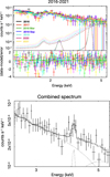 |
Fig. 2 Upper panel: Chandra/ACIS spectra extracted from the circular region shown in Fig. 1 for all observations performed between 2016 and 2021 (see Table A.1), with the corresponding best-fit model and residuals. Dotted lines show each component of the best fit model for each epochs. Lower panel: combined spectrum obtained by summing all the observations shown in the upper panel. The 44Sc line is modelled by a narrow Gaussian at 4.076 keV. Dotted lines indicate the different components of the best-fit model. |
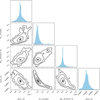 |
Fig. 3 Close-up view of the MCMC corner plot shown in Fig. D.1. The parameter norm_24 indicates the normalization of the Gaussian at 4.076 keV, not corrected for the PSF effects (see text). The parameters kT_25, Tau_39, and norm_41 correspond to the temperature, ionization parameter, and normalization, respectively, for the vnei component in the 2016 spectrum. |
4 XRISM-Resolve simulated spectra
The detection of the 44Sc line might be feasible with the new X-ray telescope, XRISM. SN 1987A will not be spatially resolved by the XRISM mirrors; therefore, it will not be possible to extract spectra from small regions to reduce contamination from thermal X-ray emission, as was done with Chandra. However, the high spectral resolution offered by the XRISM-Resolve spectrometer will facilitate detection of the line emerge over the continuum.
We simulated XRISM-Resolve spectra for the year 2025 using a phenomenological model that reproduces the spectrum from Sapienza et al. (2024a,b), including the effects of the gate valve closing. We assumed an exposure time of 400 ks, which is similar to the actual exposure time for SN 1987A in the XRSIM Performance Verification Phase observation. We added a Gaussian component to this model to account for the 44Sc line, along with an absorbed power law (Greco et al. 2021, 2022) for the year 2024 to account for the emission of the putative Pulsar Wind Nebula (PWN). Figure 4 shows the simulated spectra obtained by assuming two different 44Sc line widths (the line being Doppler-broadened because of the rapid expansion of the ejecta), namely 1000 km s−1 and 2000 km s−1, in the left and right panels, respectively.
The detectability of the line strongly depends on its broadening. For an expansion velocity of 1000 km s−1, the significance of the detection exceeds the 99% confidence level. However, assuming a much more reasonable value of 2000 km s−1 for the expansion velocity, the analysis of the synthetic spectrum shows a non-detection of the 44Sc line, with its flux being larger than zero at only the 68% confidence level. These results therefore indicate a non-detection of the 44Sc line with XRISM-Resolve, in agreement with the recent findings of XRISM collaboration (2025).
5 Discussion and conclusion
The study of 44Ti in SNRs plays a crucial role in understanding the physical processes governing the explosion of massive stars. Previous studies have detected radioactive emission lines of 44Ti in SN 1987A (Boggs et al. 2015; Grebenev et al. 2012), although NuSTAR and INTEGRAL spectra yield different fluxes, leaving the initial mass of 44Ti still under debate. In particular, using the relation between the flux and the initial mass of 44Ti, Eq. (1), a value of M44 = (1.5 ± 0.3) × 10−4M⊙ was derived from NuSTAR data (Boggs et al. 2015), while M44 = (3.1 ± 0.8) × 10−4M⊙ was obtained from INTEGRAL (Grebenev et al. 2012). Another method of measuring the initial mass of 44Ti involves the emission line of 44Sc, which is a product of the 44 Ti decay chain.
In this work, we performed a systematic search for the 44Sc line by analyzing multi-epoch Chandra observations of SN 1987A (from 2000 to 2021). We exploited the remarkable spatial resolution of the Chandra mirrors to extract X-ray spectra from a small region (radius 0.3 arcsec) in the center of the remnant, as shown in Fig. 1.
While detection of the 44Sc line is affected by absorption from the surrounding cold ejecta at early epochs (as predicted by Fransson & Chevalier 1987), we detect the 44Sc line with high significance in spectra extracted from observations performed between 2016 and 2021, when the cold ejecta are expected to be optically thin. We measure a line flux  photons s−1 cm−2, corresponding to an initial mass M44 = (1.6 ± 0.5) × 10−4M⊙. To our knowledge, this is the first firm detection of the Sc emission line in SN 1987A.
The precise estimation of the mass of 44Ti depends on the actual size and morphology of the emitting region. As described in Sect. 3, our analysis was conducted assuming the 44Sc emission as arising from a circular region of radius 0.3″. According to Larsson et al. (2023), we consider this extent an upper limit. As a result, our initial mass of 44Ti must be considered as an upper limit value. Nevertheless, we show that even by assuming a different distribution of the line surface brightness, our results do not change significantly (<10%). Our estimate of the 44Ti mass is in close agreement with the NuSTAR analysis of (Boggs et al. 2015). However, it is significantly lower than that obtained by Grebenev et al. (2012) based on INTEGRAL observations.
Our value of M44 is also in good agreement with long-term 3D simulations of neutrino-driven explosions (Sieverding et al. 2023), assuming an explosion energy of (1.3 - 1.5) × 1051 erg (Arnett 1987; Utrobin 2005; Utrobin et al. 2021; Wang & Burrows 2024).
New Chandra observations will improve the statistics and provide a more constrained estimate of M44.
In conclusion, our work provides an independent procedure for measuring the yield of 44Ti in SN 1987A by analyzing soft X-ray emission. Future observations will further tighten these constraints.
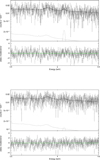 |
Fig. 4 Synthetic XRISM-Resolve spectra produced using the model by Sapienza et al. (2024a) with the addition of the expected Scandium line for the year 2025, and with updated RMF and ARF including the effects of the closed gate valve (Sapienza et al. 2024b). Dotted lines show the different components of the best-fit model. The exposure time is 400 ks. Upper panel: spectrum synthesized including the best-fit Gaussian component with a line width corresponding to a Doppler broadening of 1000 km s−1. Lower panel: same as for the upper panel, but for a Doppler broadening of 2000 km s−1. |
Acknowledgements
M.M., V.S., E.G., S.O., and F.B. acknowledge financial contribution from the PRIN 2022 (20224MNC5A) – “Life, death and afterdeath of massive stars” funded by European Union – Next Generation EU, and the INAF Theory Grant “Supernova remnants as probes for the structure and mass-loss history of the progenitor systems”. This paper is partially supported by the Fondazione ICSC, Spoke 3 Astrophysics and Cosmos Observations. National Recovery and Resilience Plan (Piano Nazionale di Ripresa e Resilienza, PNRR) Project ID CN_00000013 “Italian Research Center on High-Performance Computing, Big Data and Quantum Computing” funded by MUR Missione 4 Componente 2 Investimento 1.4: Potenziamento strutture di ricerca e creazione di “campioni nazionali di R&S (M4C2-19)” – Next Generation EU (NGEU). R.G., V.S., O.P. acknowledge partial support from the INAF mini-grant 1.05.23.04.04. This project was partially funded also through the MSCA4Ukraine project from the European Union. Views and opinions expressed are however those of the authors only and do not necessarily reflect those of the European Union. Neither the European Union nor the MSCA4Ukraine Consortium as a whole nor any individual member institutions of the MSCA4Ukraine Consortium can be held responsible for them. This work made use of the HPC system MEUSA, part of the Sistema Computazionale per l’Astrofisica Numerica (SCAN) of INAF-Osservatorio Astronomico di Palermo. S.N. is supported by JSPS Grantin-Aid Scientific Research (KAKENHI) (A), Grant Number JP25H00675 and JST ASPIRE Program “RIKEN-Berkeley mathematical quantum science initiative. We acknowledge Andrea Damonte for his kind support on the MCMC chains.
Appendix A Observations
Table A.1 lists the Chandra observations analyzed in this paper. Horizontal lines marks the different groups that we selected for the spectral analysis (see Sect. 3 and Appendix B).
Observations.
Appendix B Flux temporal evolution
Motivated by the detection of the 44Sc emission line in the 2016-2021 spectra, we repeated the spectral analysis described in Sect. 3 on earlier epochs, dividing the data into three additional groups, namely Group 1 for observations performed between 2000 and 2004, Group 2 for those in 2005 - 2009, and Group 3 for 2010 - 2015. Figure B.1 shows the spectra of the different Groups. We measure the flux of the emission line centered at 4.076 keV in all the Groups, the line flux (corrected for the PSF effects) being  photons s−1 cm−2, F2 < 3.9 × 10⁻⁸ photons s−1 cm−2,
  photons s−1 cm−2 in Group 1, Group 2, and Group 3, respectively (error bars at 90% confidence level). As expected, the line flux in Groups 1 - 3, is significantly lower than that in Group 4. This is likely the result of the cold ejecta being still optically thick at these epochs. However, discussing the time evolution of the line flux is beyond the scope of this paper, given its intrinsic complexity related to (i) the complex effect of the absorption of cold ejecta, which monotonically (but non-linearly) decreases with time, (ii) the expansion of the bright X-ray ring (which decreases the fraction of photons spilling from the ring into our extraction region); and (iii) the increase of the hard X-ray flux (3 - 8 keV; see Ravi et al. 2024), which increases the contamination from the ring.
We also checked that the line is not significantly detected in the spectra of the ring (as already shown by Leising 2006 for the first Chandra observations). As an example, we explored the spectra in 2014 and 2020 finding that the line flux is always compatible with 0 at the 68% confidence level. Figure B.2 shows that the line emission is always well below the continuum.
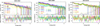 |
Fig. B.1 Chandra/ACIS spectra extracted from the circular region shown in Fig. 1 for all observations performed between 2000 and 2004 (left), 2005-2009 (center), and 2010-2015 (right) with the corresponding best-fit model and residuals. |
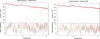 |
Fig. B.2 Spectra of the X-ray emission originating from a region including the ER of SN1987A at two different epochs – 2014 (left panel) and 2020 (right panel) – with the corresponding best fit model and residuals. |
Appendix C Background spectrum
Figure C.1 shows our choice of the background extraction region together with an example of the background spectrum, fitted with the following model:
 (C.1)
(C.1)
In all of the background spectra the best fit model includes a power law taking into account the continuum, the model apec fitting the emission spectrum from collisionally ionized diffuse gas, based on the database AtomDB version 3.09 https://heasarc.gsfc.nasa.gov/xanadu/xspec/manual/XSmodelApec.html, plus three emission lines centered at energies which are less than 3 keV.
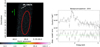 |
Fig. C.1 Left panel: Chandra/ACIS count map for Obs ID 21304 (same as in Fig. 1) in log scale. The red ellipse shows the background extraction region. Right panel: Spectrum extracted from the background region in the left panel with the corresponding best fit model (Eq. (C.1)) and residuals. |
Appendix D Corner plot
Figure D.1 presents the MCMC corner plot for the simultaneous analysis of the spectra collected between 2016 and 2021. Each panel shows the correlation between two different free parameters, indicated as parameter_number. In this case, norm_24 is the flux associated with the 44Sc emission line. All the temperature, ionization times and normalization are associated with the vnei component fitted for each spectrum.
References
- Ahmad, I., Greene, J. P., Moore, E. F., et al. 2006, Phys. Rev. C, 74, 065803 [Google Scholar]
- Alp, D., Larsson, J., & Fransson, C. 2021, ApJ, 916, 76 [NASA ADS] [CrossRef] [Google Scholar]
- Arnaud, K. A. 1996, in Astronomical Society of the Pacific Conference Series, 101, Astronomical Data Analysis Software and Systems V, eds. G. H. Jacoby, & J. Barnes, 17 [Google Scholar]
- Arnett, W. D. 1987, ApJ, 319, 136 [Google Scholar]
- Arnett, W. D., Bahcall, J. N., Kirshner, R. P., & Woosley, S. E. 1989, ARA&A, 27, 629 [NASA ADS] [CrossRef] [Google Scholar]
- Basko, M. 1994, ApJ, 425, 264 [NASA ADS] [CrossRef] [Google Scholar]
- Beuermann, K., Brandt, S., & Pietsch, W. 1994, A&A, 281, L45 [NASA ADS] [Google Scholar]
- Boggs, S. E., Harrison, F. A., Miyasaka, H., et al. 2015, Science, 348, 670 [Google Scholar]
- Borkowski, K. J., Reynolds, S. P., Green, D. A., et al. 2010, ApJ, 724, L161 [NASA ADS] [CrossRef] [Google Scholar]
- Burrows, C. J., Krist, J., Hester, J. J., et al. 1995, ApJ, 452, 680 [NASA ADS] [CrossRef] [Google Scholar]
- Cash, W. 1979, ApJ, 228, 939 [Google Scholar]
- Chevalier, R. A., & Dwarkadas, V. V. 1995, ApJ, 452, L45 [Google Scholar]
- Colgan, S. W. J., Haas, M. R., Erickson, E. F., Lord, S. D., & Hollenbach, D. J. 1994, ApJ, 427, 874 [Google Scholar]
- Cook, W. R., Palmer, D. M., Prince, T. A., et al. 1988, ApJ, 334, L87 [Google Scholar]
- Davis, J. E., Bautz, M. W., Dewey, D., et al. 2012, SPIE Conf. Ser., 8443, 84431A [NASA ADS] [Google Scholar]
- Dotani, T., Hayashida, K., Inoue, H., et al. 1987, Nature, 330, 230 [Google Scholar]
- Frank, K. A., Zhekov, S. A., Park, S., et al. 2016, ApJ, 829, 40 [Google Scholar]
- Fransson, C., & Chevalier, R. A. 1987, ApJ, 322, L15 [NASA ADS] [CrossRef] [Google Scholar]
- Grebenev, S. A., Lutovinov, A. A., Tsygankov, S. S., & Winkler, C. 2012, Nature, 490, 373 [Google Scholar]
- Greco, E., Miceli, M., Orlando, S., et al. 2021, ApJ, 908, L45 [NASA ADS] [CrossRef] [Google Scholar]
- Greco, E., Miceli, M., Orlando, S., et al. 2022, ApJ, 931, 132 [Google Scholar]
- Haas, M. R., Colgan, S. W. J., Erickson, E. F., et al. 1990, ApJ, 360, 257 [NASA ADS] [CrossRef] [Google Scholar]
- Haberl, F., Geppert, U., Aschenbach, B., & Hasinger, G. 2006, A&A, 460, 811 [NASA ADS] [CrossRef] [EDP Sciences] [Google Scholar]
- Hashimoto, M. 1995, Progr. Theor. Phys., 94, 663 [Google Scholar]
- Helder, E. A., Broos, P. S., Dewey, D., et al. 2013, ApJ, 764, 11 [Google Scholar]
- Jerkstrand, A., Fransson, C., & Kozma, C. 2011, A&A, 530, A45 [NASA ADS] [CrossRef] [EDP Sciences] [Google Scholar]
- Kaastra, J. S., & Bleeker, J. A. M. 2016, A&A, 587, A151 [NASA ADS] [CrossRef] [EDP Sciences] [Google Scholar]
- Kifonidis, K., Plewa, T., Janka, H. T., & Müller, E. 2003, A&A, 408, 621 [NASA ADS] [CrossRef] [EDP Sciences] [Google Scholar]
- Larsson, J., Fransson, C., Spyromilio, J., et al. 2016, ApJ, 833, 147 [NASA ADS] [CrossRef] [Google Scholar]
- Larsson, J., Fransson, C., Sargent, B., et al. 2023, ApJ, 949, L27 [NASA ADS] [CrossRef] [Google Scholar]
- Leising, M. D. 2006, ApJ, 651, 1019 [Google Scholar]
- Leising, M. D., & Share, G. H. 1990, ApJ, 357, 638 [NASA ADS] [CrossRef] [Google Scholar]
- Lundqvist, P., & Fransson, C. 1991, ApJ, 380, 575 [Google Scholar]
- Luo, D., & McCray, R. 1991, in Bulletin of the American Astronomical Society, 23, 1406 [Google Scholar]
- Magkotsios, G., Timmes, F. X., Hungerford, A. L., et al. 2010, ApJS, 191, 66 [NASA ADS] [CrossRef] [Google Scholar]
- Mahoney, W. A., Varnell, L. S., Jacobson, A. S., et al. 1988, ApJ, 334, L81 [Google Scholar]
- Maitra, C., Haberl, F., Sasaki, M., et al. 2022, A&A, 661, A30 [NASA ADS] [CrossRef] [EDP Sciences] [Google Scholar]
- Mao, J., Ono, M., Nagataki, S., et al. 2015, ApJ, 808, 164 [Google Scholar]
- Matz, S. M., Share, G. H., Leising, M. D., et al. 1988, Nature, 331, 416 [NASA ADS] [CrossRef] [Google Scholar]
- Miceli, M. 2023, Plasma Phys. Controlled Fusion, 65, 034003 [Google Scholar]
- Miceli, M., Orlando, S., Burrows, D. N., et al. 2019, Nat. Astron., 3, 236 [Google Scholar]
- Nagataki, S. 2000, ApJS, 127, 141 [NASA ADS] [CrossRef] [Google Scholar]
- Nagataki, S., Hashimoto, M.-a., Sato, K., & Yamada, S. 1997, ApJ, 486, 1026 [Google Scholar]
- Nagataki, S., Hashimoto, M.-a., Sato, K., Yamada, S., & Mochizuki, Y. S. 1998, ApJ, 492, L45 [Google Scholar]
- Ono, M., Nagataki, S., Ferrand, G., et al. 2020, ApJ, 888, 111 [NASA ADS] [CrossRef] [Google Scholar]
- Orlando, S., Miceli, M., Pumo, M. L., & Bocchino, F. 2015, ApJ, 810, 168 [NASA ADS] [CrossRef] [Google Scholar]
- Orlando, S., Miceli, M., Petruk, O., et al. 2019, A&A, 622, A73 [NASA ADS] [CrossRef] [EDP Sciences] [Google Scholar]
- Orlando, S., Ono, M., Nagataki, S., et al. 2020, A&A, 636, A22 [NASA ADS] [CrossRef] [EDP Sciences] [Google Scholar]
- Orlando, S., Miceli, M., Ono, M., et al. 2025, A&A, 699, A305 [NASA ADS] [CrossRef] [EDP Sciences] [Google Scholar]
- Panagia, N. 1999, in New Views of the Magellanic Clouds, 190, ed. Y. H. Chu, N. Suntzeff, J. Hesser, & D. Bohlender, 549 [Google Scholar]
- Park, S., Burrows, D. N., Garmire, G. P., Zhekov, S. A., & McCray, R. 2006, in The Tenth Marcel Grossmann Meeting. On recent developments in theoretical and experimental general relativity, gravitation and relativistic field theories, 1281 [Google Scholar]
- Ravi, A. P., Park, S., Zhekov, S. A., et al. 2021, ApJ, 922, 140 [Google Scholar]
- Ravi, A. P., Park, S., Zhekov, S. A., et al. 2024, ApJ, 966, 147 [Google Scholar]
- Sandie, W. G., Nakano, G. H., Chase, L. F., et al. 1988, in American Institute of Physics Conference Series, 170, Nuclear Spectroscopy of Astrophysical Sources, eds. N. Gehrels & G. H. Share (AIP), 66 [Google Scholar]
- Sapienza, V., Miceli, M., Bamba, A., et al. 2024a, ApJ, 961, L9 [Google Scholar]
- Sapienza, V., Miceli, M., Bamba, A., et al. 2024b, RNAAS, 8, 156 [Google Scholar]
- Sieverding, A., Kresse, D., & Janka, H.-T. 2023, ApJ, 957, L25 [NASA ADS] [CrossRef] [Google Scholar]
- Sun, L., Vink, J., Chen, Y., et al. 2021, ApJ, 916, 41 [NASA ADS] [CrossRef] [Google Scholar]
- Teegarden, B. J., Barthelmy, S. D., Gehrels, N., Tueller, J., & Leventhal, M. 1989, Nature, 339, 122 [Google Scholar]
- Thielemann, F.-K., Hashimoto, M.-A., & Nomoto, K. 1990, ApJ, 349, 222 [CrossRef] [Google Scholar]
- Urushibata, T., Takahashi, K., Umeda, H., & Yoshida, T. 2018, MNRAS, 473, L101 [CrossRef] [Google Scholar]
- Utrobin, V. P. 2005, Astron. Lett., 31, 806 [NASA ADS] [CrossRef] [Google Scholar]
- Utrobin, V. P., Chugai, N. N., & Andronova, A. A. 1995, A&A, 295, 129 [NASA ADS] [Google Scholar]
- Utrobin, V. P., Wongwathanarat, A., Janka, H. T., et al. 2021, ApJ, 914, 4 [NASA ADS] [CrossRef] [Google Scholar]
- Wang, T., & Burrows, A. 2024, ApJ, 974, 39 [Google Scholar]
- West, R. M. 1987, Mercury, 16, 80 [Google Scholar]
- Woosley, S. E., & Hoffman, R. D. 1991, ApJ, 368, L31 [Google Scholar]
- XRISM collaboration 2025, PASJ, in press [Google Scholar]
All Tables
All Figures
|
Fig. 1 Upper panel: Chandra/ ACIS photon count map of SN 1987A in 2019 (Obs ID 21304), in the 0.5–7.0 keV energy band. Lower panel: same image as above, but deconvolved using the Lucy-Richardson algorithm. Both images have a pixel size of 0.06″. The red circle indicates the region selected for spectral analysis. |
| In the text | |
|
Fig. 2 Upper panel: Chandra/ACIS spectra extracted from the circular region shown in Fig. 1 for all observations performed between 2016 and 2021 (see Table A.1), with the corresponding best-fit model and residuals. Dotted lines show each component of the best fit model for each epochs. Lower panel: combined spectrum obtained by summing all the observations shown in the upper panel. The 44Sc line is modelled by a narrow Gaussian at 4.076 keV. Dotted lines indicate the different components of the best-fit model. |
| In the text | |
|
Fig. 3 Close-up view of the MCMC corner plot shown in Fig. D.1. The parameter norm_24 indicates the normalization of the Gaussian at 4.076 keV, not corrected for the PSF effects (see text). The parameters kT_25, Tau_39, and norm_41 correspond to the temperature, ionization parameter, and normalization, respectively, for the vnei component in the 2016 spectrum. |
| In the text | |
|
Fig. 4 Synthetic XRISM-Resolve spectra produced using the model by Sapienza et al. (2024a) with the addition of the expected Scandium line for the year 2025, and with updated RMF and ARF including the effects of the closed gate valve (Sapienza et al. 2024b). Dotted lines show the different components of the best-fit model. The exposure time is 400 ks. Upper panel: spectrum synthesized including the best-fit Gaussian component with a line width corresponding to a Doppler broadening of 1000 km s−1. Lower panel: same as for the upper panel, but for a Doppler broadening of 2000 km s−1. |
| In the text | |
|
Fig. B.1 Chandra/ACIS spectra extracted from the circular region shown in Fig. 1 for all observations performed between 2000 and 2004 (left), 2005-2009 (center), and 2010-2015 (right) with the corresponding best-fit model and residuals. |
| In the text | |
|
Fig. B.2 Spectra of the X-ray emission originating from a region including the ER of SN1987A at two different epochs – 2014 (left panel) and 2020 (right panel) – with the corresponding best fit model and residuals. |
| In the text | |
|
Fig. C.1 Left panel: Chandra/ACIS count map for Obs ID 21304 (same as in Fig. 1) in log scale. The red ellipse shows the background extraction region. Right panel: Spectrum extracted from the background region in the left panel with the corresponding best fit model (Eq. (C.1)) and residuals. |
| In the text | |
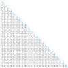 |
Fig. D.1 MCMC Corner plot for the simultaneous fit of 2016-2021 spectra (see Sects. 2 and 3). |
| In the text | |
Current usage metrics show cumulative count of Article Views (full-text article views including HTML views, PDF and ePub downloads, according to the available data) and Abstracts Views on Vision4Press platform.
Data correspond to usage on the plateform after 2015. The current usage metrics is available 48-96 hours after online publication and is updated daily on week days.
Initial download of the metrics may take a while.