| Issue |
A&A
Volume 700, August 2025
|
|
|---|---|---|
| Article Number | A128 | |
| Number of page(s) | 11 | |
| Section | Cosmology (including clusters of galaxies) | |
| DOI | https://doi.org/10.1051/0004-6361/202555719 | |
| Published online | 11 August 2025 | |
CHEX-MATE: The impact of triaxiality and orientation on Planck SZ cluster selection and weak lensing mass measurements
1
California Institute of Technology, 1200 East California Boulevard, Pasadena, California, USA
2
IRFU, CEA, Université Paris-Saclay, 91191 Gif-sur-Yvette, France
3
Smithsonian Astrophysical Observatory, Cambridge, Massachusetts, USA
4
Department of Physics, Korea Advanced Institute of Science and Technology (KAIST), 291 Daehak-ro, Yuseong-gu, Daejeon 34141, Republic of Korea
5
Université Paris-Saclay, Université Paris Cité, CEA, CNRS, AIM, 91191 Gif-sur-Yvette, France
6
INAF – Osservatorio di Astrofisica e Scienza dello Spazio di Bologna, Via Piero Gobetti 93/3, I-40129 Bologna, Italy
7
INFN, Sezione di Bologna, Viale Berti Pichat 6/2, I-40127 Bologna, Italy
8
INAF, Istituto di Astrofisica Spaziale e Fisica Cosmica di Milano, Via A. Corti 12, 20133 Milano, Italy
9
Center for Astrophysics | Harvard & Smithsonian, 60 Garden Street, Cambridge, MA 02138, USA
10
IRAP, CNRS, Université de Toulouse, CNES, Toulouse, France
11
INFN-Sezione di Genova, Via Dodecaneso 33, 16146 Genova, Italy
12
Department of Physics, Informatics and Mathematics, University of Modena and Reggio Emilia, 41125 Modena, Italy
13
Dipartimento di Fisica, Sapienza Università di Roma, Piazzale Aldo Moro 5, I-00185 Rome, Italy
14
INAF, Osservatorio Astronomico di Trieste, Via Tiepolo 11, I-34131 Trieste, Italy
15
IFPU, Institute for Fundamental Physics of the Universe, Via Beirut 2, 34014 Trieste, Italy
16
Department of Physics; University of Michigan, Ann Arbor, MI 48109, USA
17
Department of Astronomy, University of Geneva, Ch. d’Ecogia 16, CH-1290 Versoix, Switzerland
18
Jodrell Bank Centre for Astrophysics, Department of Physics and Astronomy, The University of Manchester, Manchester M13 9PL, UK
19
HH Wills Physics Laboratory, University of Bristol, Bristol, UK
⋆ Corresponding author.
Received:
29
May
2025
Accepted:
10
June
2025
Abstract
Context. Galaxy cluster abundance measurements are a valuable tool for constraining cosmological parameters, such as the mass density (Ωm) and the density fluctuation amplitude (σ8). Wide-area surveys detect clusters based on observables, such as the total integrated Sunyaev-Zel’dovich effect signal (YSZ) in the case of Planck. Quantifying the survey selection function is necessary for cosmological analyses, with completeness representing the probability of detecting a cluster as a function of its intrinsic properties, such as YSZ and an angular scale θ500.
Aims. We determine the completeness of the Planck-selected CHEX-MATE cluster catalog using mock observations of clusters with triaxial shapes and random orientations, with physically-motivated distributions of axial ratios. From these mocks, we derive the distribution of shapes and orientations of the detected clusters, along with any associated bias in weak-lensing-derived mass (MWL) due to this orientation-dependent selection (denoted as 1 − bχ).
Methods. Employing a Monte Carlo method, we injected triaxial cluster profiles into random positions within the Planck all-sky maps and subsequently determined the completeness as a function of both geometry and SZ brightness. This result was then used to generate 1000 mock CHEX-MATE cluster catalogs. We computed MWL for these mock CHEX-MATE clusters and for equal-sized samples of randomly selected clusters with similar mass and redshift distributions.
Results. Cluster orientation impacts completeness, with a higher probability of detecting clusters elongated along the line of sight (LOS). This leads to 1 − bχ values of 0−4% for CHEX-MATE clusters relative to a random population. The largest increase in MWL is observed in the lowest-mass objects, which are most impacted by orientation-related selection bias.
Conclusions. Clusters in Planck SZ-selected catalogs are preferentially elongated along the LOS and have an average bias in MWL relative to randomly selected cluster samples. This bias is relevant for upcoming SZ surveys such as CMB-S4, and should be considered for surveys utilizing other probes for cluster detection, such as Euclid.
Key words: gravitational lensing: weak / galaxies: clusters: general / galaxies: clusters: intracluster medium / cosmology: observations
© The Authors 2025
 Open Access article, published by EDP Sciences, under the terms of the Creative Commons Attribution License (https://creativecommons.org/licenses/by/4.0), which permits unrestricted use, distribution, and reproduction in any medium, provided the original work is properly cited.
This article is published in open access under the Subscribe to Open model. This email address is being protected from spambots. You need JavaScript enabled to view it. to support open access publication.
1. Introduction
Galaxy cluster abundance is a powerful cosmological probe, offering incisive tests of the ΛCDM model and precise measurements of fundamental cosmological parameters (e.g., Voit 2005; Allen et al. 2011; Lesci et al. 2022a). As the most massive gravitationally bound structures in the Universe, galaxy clusters trace the late stages of structure formation, representing the evolution of the highest peaks in the primordial matter density field (Despali et al. 2016). Their abundance is particularly useful for constraining both the mean matter density (Ωm) and the amplitude of matter fluctuations (σ8), defined as the root mean square (rms) of linear density perturbations on scales of 8 h−1 Mpc. Recent studies using cluster catalogs selected from X-ray, optical, and millimeter-wavelength surveys have yielded increasingly precise constraints on these parameters (Ghirardini et al. 2024; DES Collaboration 2025; Bocquet et al. 2024), although challenges related to halo mass calibration and selection biases still remain.
The hot intracluster medium (ICM) emits X-rays via thermal bremsstrahlung (Sarazin 1986), producing a bright, diffuse signal that makes X-ray surveys a valuable tool for detecting galaxy clusters. Early X-ray halo abundance studies were based on catalogs of approximately 100 clusters detected in the ROSAT All-Sky Survey (RASS), using deep X-ray follow-up from Chandra to determine halo masses via hydrostatic equilibrium-based estimates (Vikhlinin et al. 2009; Mantz et al. 2010). Because the bias associated with such mass estimates is difficult to quantify, later work improved on these results by utilizing weak-lensing (WL) observations of a subsample of clusters to calibrate the halo mass scale (Mantz et al. 2015). The more recent XXL survey from XMM-Newton, which is much narrower and deeper than the RASS, delivered a comparably sized cluster sample with WL again calibrating the mass scale for a halo abundance measurement (Pacaud et al. 2018). The current state of the art in X-ray cluster cosmology was obtained from the eROSITA (extended ROentgen Survey with an Imaging Telescope Array) All-Sky Survey (eRASS), based on over 5000 X-ray-selected clusters (Ghirardini et al. 2024). Cluster masses were calibrated using WL, in this case using WL mass (MWL) estimates from three different optical surveys (Chiu et al. 2022; Kleinebreil et al. 2025; Grandis et al. 2024), enabling a robust scaling between X-ray observables and total halo mass (see also Okabe et al. 2025).
In the optical regime, cluster detection is most often based on searching for overdensities of galaxies, for example, using algorithms that attempt to identify a red sequence of cluster-member galaxies (e.g., Rykoff et al. 2014; Bellagamba et al. 2017). For instance, commensurate with the RASS-based studies noted above, the maxBCG cluster sample from the Sloan Digital Sky Survey (SDSS) was used by Rozo et al. (2010) to derive cosmological constraints from over 104 clusters and groups at low redshifts. To connect the detection observable, optical richness, with the underlying halo mass, stacked MWL values within bins of fixed richness were used. Subsequent work by Costanzi et al. (2019) combines abundance and WL measurements from the SDSS DR8 to jointly constrain cosmology and the richness–mass relation for a photometrically selected sample of red-sequence Matched-filter Probabilistic Percolation (redMaPPer) clusters. Illustrating the challenges related to selection and mass calibration, the Dark Energy Survey (DES) released its initial halo abundance measurement soon after (Abbott et al. 2020), with an anomalously low value of the matter density that was later found to be due to biases in MWL values for the lowest-richness clusters (To et al. 2021; Costanzi et al. 2021). The current state of the art in optical cluster cosmology is presented in the DES Y3 results and the third release of the Kilo-Degree Survey (DES Collaboration 2025; Lesci et al. 2022b), who find cosmological parameter values that are fully consistent with those obtained from primary CMB anisotropy measurements from Planck.
Scattering of CMB photons with electrons in the ICM produces an average boost in photon energy known as the Sunyaev-Zel’dovich (SZ) effect (Sunyaev & Zeldovich 1972), which enables the detection of clusters in millimeter-wave surveys. Recent large-area surveys from the Atacama Cosmology Telescope (Hilton et al. 2021), the South Pole Telescope (Bleem et al. 2015, 2024; Kornoelje et al. 2025), and Planck (Planck Collaboration XXVII 2016, hereafter P16) have now provided catalogs with thousands of clusters, which have in turn been used to constrain cosmological parameters (Sehgal et al. 2011; Bocquet et al. 2024; Planck Collaboration XXIV 2016). Notably, the SZ effect surface brightness is independent of redshift, making these surveys approximately mass-limited across most redshifts, and thus providing catalogs that areparticularly attractive for halo abundance measurements. However, results from these surveys are generally limited by systematic uncertainties in halo mass calibration. For example, Planck detected fewer clusters than predicted by the base ΛCDM model, as constrained by its primary CMB anisotropy measurement, when hydrostatic mass estimates are used for the cluster measurement (Planck Collaboration XXIV 2016; Planck Collaboration VI 2020). This discrepancy motivated numerous WL studies to improve the mass calibration (e.g., von der Linden et al. 2014; Hoekstra et al. 2015), although most of these calibrations still suggest at least mild tension between the cluster and CMB measurements.
As noted above, a central challenge in cluster cosmology, both for halo abundance and clustering, is accurately calibrating the scaling relations between mass and observables–such as X-ray brightness, optical richness, and SZ flux (YSZ)–which are needed to connect cluster detections based on these observables to the Halo Mass Function (HMF). In general, systematic uncertainties in this calibration limit the precision of the derived cosmological constraints (e.g., Pratt et al. 2019). To improve mass calibration, nearly all recent efforts focus on MWL, which is sensitive to the total projected mass distribution and is independent of the dynamical state of the ICM. However, MWL values exhibit significant cluster-to-cluster scatter, along with an average bias, primarily from projection effects due to halo asphericity, orientation, and miscentering (e.g., Meneghetti et al. 2010; Giocoli et al. 2025; Euclid Collaboration: Ragagnin et al. 2025). To quantify this scatter and bias, researchers commonly perform mock WL analyses of simulated clusters with random orientations (e.g., Euclid Collaboration: Giocoli et al. 2024). A limitation of such studies arises if the observable used to detect the cluster sample is sensitive to halo orientation, resulting in a selected population with a preferred geometry. In this case, the scatter and bias in MWL could be misestimated.
Understanding the selected population of galaxy clusters requires quantifying survey completeness, which measures the probability of detecting a cluster based on its observables. For the Planck SZ survey, completeness, χ(Y5R500, θ500, l, b), is defined as a function of four cluster parameters, where Y5R500 is the integrated SZ signal within 5R500, θ500 is the corresponding angular scale, and (l, b) are the cluster’s galactic coordinates (P16)1. Detectability is assessed using the observed signal-to-noise ratio (S/N) obtained from, e.g., the Multi-Matched Filtering (MMF3) algorithm (P16, see also Melin et al. 2006, 2012), which must exceed a threshold value. A robust Monte Carlo (MC) method for characterizing completeness involves injecting a large number of model clusters with a range of values for Y5R500 and θ500 into random locations within the Planck maps, then computing the S/N from the MMF3 for each injected cluster. The Planck team did not consider asphericity in this calculation and injected clusters based only on spherically symmetric models. Subsequent work by Gallo et al. (2024) estimated the Planck completeness using simulated clusters with complicated aspherical shapes more closely resembling reality, finding that steeper SZ signal profiles yield a higher probability of detection. The impact of halo ellipticity was minimal. Overall, the change in completeness obtained by Gallo et al. (2024) results in approximately 1σ shifts in the derived values of Ωm and σ8 relative to the nominal Planck result.
In this work, we provide a formalism to investigate how halo triaxiality and orientation impact cluster detection and SZ selection, focusing on the Planck-selected Cluster HEritage project with Mass Assembly and Thermodynamics at the Endpoint of structure formation (CHEX-MATE) sample. By utilizing smooth cluster models, rather than the simulated clusters of Gallo et al. (2024), we isolate the impact of triaxiality and orientation from other characteristics such as substructure and dynamical state. In addition, because our study is not limited to a relatively small number of simulated objects, we are also able to obtain sufficient statistics to characterize sub-percent level biases. The CHEX-MATE project (CHEX-MATE Collaboration 2021) is an XMM-Newton Heritage Project designed to study ICM physics and improve cluster-based cosmological constraints by refining links between observables and halo mass2. It includes 118 clusters, divided into a volume-limited sample (Tier 1, 0.05 < z < 0.2) and a mass-limited sample (Tier 2, z < 0.6, M > 7.25 × 10¹⁴ M⊙), each containing 61 clusters, with four clusters in common. Furthermore, all clusters in the catalog have a Planck S/N > 6.5, and Tier 1 is restricted to the northern sky, Dec > 0°. This deep, uniform, and high-quality multi-probe dataset enables precise measurements of triaxial 3D cluster shapes and orientations (Kim et al. 2024). Our goal is to model the SZ selection function of the CHEX-MATE sample while incorporating cluster triaxiality through informative priors. The end result is a CHEX-MATE completeness estimate that depends on the triaxial geometry, along with a determination of the expected distribution of the geometries for the CHEX-MATE sample. We further explore the impact of this selection on the values of MWL derived for the CHEX-MATE clusters.
This paper is organized as follows. In Section 2, we describe the details of the MMF3 algorithm used to compute cluster detection and selection. In Section 3, we describe the triaxial model assumed for the ICM and the total mass distribution of the clusters. In Section 4, we describe the MC injection and detection procedure used to calculate the completeness for a set of both spherical and triaxial clusters, and we quantify how the completeness depends on the triaxial shape and orientation parameters. In Section 5, we discuss the algorithm for generating a mock CHEX-MATE catalog, beginning with assembling a mock cluster sample from an HMF, injecting triaxial clusters from this sample based on informative priors on their shape and orientation, and subsequently detecting these mock clusters using the MMF3 algorithm. In Section 6, we estimate MWL for these mock CHEX-MATE samples to quantify any WL mass bias, defined as 1 − bWL = MWL/Mtrue, due to preferentially selected shapes and orientations. Finally, in Section 7, we summarize the main results of this work.
All of the code developed for this work, and some of the data products generated are publicly available at this link.
2. Multi-Matched filtering (MMF3) algorithm
The CHEX-MATE sample was selected from the Planck PSZ2 catalog, and we thus follow P16 in their construction of the MMF3. We independently recreated the MMF3 algorithm, with an implementation as close as possible to that used by Planck, with our verification of this implementation detailed below.
The total signal in the Planck maps at each of the High Frequency Instrument (HFI) frequencies at a given position in the sky is modeled as
 (1)
(1)
where x is the 2D pixel coordinate within the map, n(x) is the unwanted astrophysical signals and instrumental noise, and tθs(x) is the SZ signal from a cluster with angular size θs and Comptonization parameter y0 = kσT∫neTedl/(mec2). To obtain this SZ signal profile, we constructed the normalized cluster profile, τθs, which is described by the Generalized Navarro-Frank-White (GNFW) pressure profile (Nagai et al. 2007; Arnaud et al. 2010):
![Mathematical equation: $$ \begin{aligned} \tau (X) = \frac{P_0}{(c_{500}*X)^\gamma [1+(c_{500}*X)^\alpha ]^{(\beta -\gamma )/\alpha }}, \end{aligned} $$](/articles/aa/full_html/2025/08/aa55719-25/aa55719-25-eq2.gif) (2)
(2)
with P0 giving the amplitude, c500 = 1.177, α = 1.0510, β = 5.490, and γ = 0.3081. Here, X = θ/θ500, where θ is the angular radius and θs = θ500/c500. This 3D profile was then integrated along the LOS to give the projected 2D signal. This 2D map was then convolved with the Planck beam in each HFI channel, bi, which is assumed to have Gaussian profiles as given in P16, with the final observed SZ signal given by
. \end{aligned} $$](/articles/aa/full_html/2025/08/aa55719-25/aa55719-25-eq3.gif) (3)
(3)
The spectral shape of the SZ signal is
![Mathematical equation: $$ \begin{aligned} j_\nu (x_\nu ) = x_\nu T_{\mathrm{CMB} } \left[\frac{e^{x_\nu }+1}{e^{x_\nu }-1} - 4\right], \end{aligned} $$](/articles/aa/full_html/2025/08/aa55719-25/aa55719-25-eq4.gif) (4)
(4)
where  is the dimensionless frequency. Following P16, we do not consider here the effect of relativistic corrections to the SZ effect. For MMF3, we applied the detection algorithm to square cutouts of the all-sky maps centered on the cluster position, with sides of 2.5°. The noise matrix was estimated directly from these local maps, by mean-subtracting the maps, applying a Hanning window to ensure periodicity at the map edges, and then computing the cross-power spectra for the 6 × 6 Planck HFI frequencies. An azimuthal averaging procedure was applied, and then this cross-channel matrix was inverted for each Fourier-space pixel, k, defining the inverse noise covariance matrix, P−1(k). The uncertainty on the SZ signal detection was then estimated from
![Mathematical equation: $$ \begin{aligned} \sigma _{\theta _s} = \left[\sum _k \boldsymbol{t_{\theta _s}(k)} \boldsymbol{P^{-1} (k)} \boldsymbol{t_{\theta _s}(k)}\right]^{-1/2}. \end{aligned} $$](/articles/aa/full_html/2025/08/aa55719-25/aa55719-25-eq6.gif) (5)
(5)
The multi-matched filter assumes the spatial and spectral form for the SZ signal defined above. The filter (Ψθs) is uniquely specified by demanding a minimum variance estimate (Melin et al. 2006), and constructed as
 (6)
(6)
These are circularly symmetric filters and show typical Fourier ringing, as demonstrated in Melin et al. (2006), as a result of down-weighting the large angular scale modes contaminated by primary CMB anisotropy and dust. The filter uses both spatial and frequency weighting to optimally extract the cluster signal from the maps. This allowed us to recover an estimate of the signal, quantified by the central Comptonization parameter as
 (7)
(7)
and thus, finally, measuring the S/N of the cluster as  .
.
To verify our implementation of the MMF3 algorithm relative to the one utilized by P16, we compared our derived S/N values and integrated SZ signals to their published results for the CHEX-MATE sample. To do this, we first obtained 2.5° ×2.5° cutouts centered on the MMF3 position reported in P16 for each CHEX-MATE cluster from the six all-sky HFI channel Planck maps. We then applied Ψθs to each of these maps, with the angular scale of the filter spanning θs values between 0.8′ and 32′. We defined the cluster size as the filter scale that maximizes the S/N at the location of the cluster, and the best-fit SZ signal was given by the corresponding  parameter. The integrated signal within a radial extent of 5R500 was then defined as
 (8)
(8)
Figure 1 shows a comparison of our derived values of S/N for the CHEX-MATE sample to those obtained from P16. On average, we find very good agreement, with slight differences due to inherent instabilities in the MMF3 algorithm. At large angular scales, corresponding to small values of |k|, the primary CMB anisotropy dominates the lower frequency HFI maps. Since this signal is coherent across frequencies, it introduces strong inter-channel correlations in the noise. Similarly, in the high frequency HFI maps, Galactic dust emission becomes the dominant signal, and this emission is also spatially coherent and highly correlated across these frequencies. Due to these large correlations, even minor differences in how the noise is modeled can propagate nonlinearly when inverting the noise covariance matrix, resulting in measurable discrepancies in the final S/N. These discrepancies can be quantified by the difference between S/N values obtained from our MMF3 implementation and the one utilized by P16. For the CHEX-MATE sample, the median difference is 0.21, with a standard deviation of 0.72, see Fig. 1. Compared to a Gaussian distribution with this mean and scale factor, a Kolmogorov-Smirnov (KS) test yields a p-value of 0.56, indicating that the observed difference in S/N is consistent with this distribution. We note that this level of agreement is approximately a factor of two better than that found between the detection algorithms described in P16, suggesting that our implementation of the MMF3 is consistent with the one utilized by P16. Furthermore, applying our MMF3 algorithm results in only three out of 118 CHEX-MATE clusters falling below the detection threshold of S/N > 6.5. As a result, we expect the overall impact on sample selection from our MMF3 implementation relative to that of P16, to be minimal.
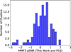 |
Fig. 1. Histogram of the difference in S/N obtained from our implementation of the MMF3 detection algorithm and that used by P16 for the CHEX-MATE clusters. |
3. Triaxial cluster shapes
The matter distribution within galaxy clusters is better approximated by a triaxial ellipsoid than by a sphere (Despali et al. 2014; Bonamigo et al. 2015; Vega-Ferrero et al. 2017), primarily due to the anisotropic accretion of matter along cosmic filaments and the complex dynamics of structure formation. Simulations suggest that modeling clusters as 3D triaxial ellipsoids results in lower bias and less intrinsic scatter in estimating intrinsic quantities (Becker & Kravtsov 2011). Observations also strongly support the triaxial nature of galaxy clusters. Ellipticity has been detected in a variety of observational probes: X-ray surface brightness maps reveal elongated morphologies (Lau et al. 2012), SZ maps show asymmetric pressure distributions (Sayers et al. 2011), and weak lensing reconstructions uncover elliptical mass distributions (Oguri et al. 2012), among others. These complementary data sets highlight the motivation for 3D triaxial modeling in both theoretical and observational contexts. As examples of such modeling, Limousin et al. (2013) present a general parametric framework within a triaxial basis to simultaneously fit complementary data sets from X-ray, SZ and lensing, and Sereno et al. (2018) demonstrate cluster shape constraints from a multi-probe 3D analysis of the X-ray regular Cluster Lensing and Supernova survey with Hubble (CLASH) clusters, using a combined analysis of strong and weak lensing, X-ray photometry and spectroscopy, and SZ.
Following these works, we assumed a geometry described by a triaxial ellipsoid with the ICM pressure following a distribution given by a radial profile in this triaxial basis, consistent with the formalism described in Kim et al. (2024). The main parameters involved in the construction of this profile are related to the intrinsic versus observed coordinate system of a triaxial ellipsoid. The projection of the ellipsoid on the sky plane is defined by an ellipse with a semi-major axis lp1 and eccentricity qp, while the projection of the ellipsoid along the LOS is defined by a semi-axis llos. The parameters lp1, qp, and llos have complicated descriptions in terms of the viewing angle and geometry of the ellipsoid (q1, q2, cos θ, ϕ, ψ), where q1 and q2 are the minor-to-major and intermediate-to-major axial ratios of the ellipsoid, respectively, with the angles defined as the Euler angles between the intrinsic and observed coordinate system. These are shown in Fig. 2 for clarity.
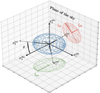 |
Fig. 2. Triaxial ellipsoid model used in the analysis. The intrinsic coordinate system of the ellipsoid is indicated by the dotted arrows, and the black arrows correspond to the observer’s coordinate system. The red ellipse shows the projection of the ellipsoid on the sky plane, with lp1 as its semi-major axis. The green ellipse shows the projection of the ellipsoid onto the plane perpendicular to the sky plane, and llos is the half size of the ellipse along the observer line of sight (Kim et al. 2024). |
We modeled the pressure as a radial profile in the elliptical basis parameterized by the ellipsoidal radius ζ, where ζ2 = (x1/q1)2 + (x2/q2)2 + x32, which is used in place of the spherical radius in the GNFW model given in Eq. (2). Within this framework, the 2D maps were calculated from the 3D ellipsoidal model projected onto the sky plane. The model Compton-y parameter is
 (9)
(9)
where y has been described in terms of the elliptical radius on the sky xξ2 = (x12+(x2/qp)2)(ls/lp1)2, xζ = ζ/ls, qp is the minor-to-major axial ratio of the observed projected isophote, ls is the semi-major axis of the ellipsoid, e∥ = llos/lp1 is the elongation parameter of the ellipsoid and Pe is obtained from the GNFW profile
![Mathematical equation: $$ \begin{aligned} P_e(x_\zeta )=\frac{P_0 P_{500}}{\left(c_{500} x_\zeta \frac{l_s}{R_{500}}\right)^{\gamma _p}\left[1+\left(c_{500} x_\zeta \frac{l_s}{R_{500}}\right)^{\alpha _p}\right]^{\left(\beta _p-\gamma _p\right)/\alpha _p}}, \end{aligned} $$](/articles/aa/full_html/2025/08/aa55719-25/aa55719-25-eq13.gif) (10)
(10)
with the same GNFW profile parameters as used in Eq. (2). Thus, a 3D triaxial model of a cluster was generated and then projected into a 2D map based on its geometrical shape parameters (q1, q2, cos θ, ϕ, ψ) and its pressure given by the GNFW model.
We defined the total SZ signal Y5R500 and angular extent θ500 for a triaxial cluster by computing the spherically-averaged radial profile of the 3D triaxial model. The spherical GNFW model was then fit to this spherically-averaged profile model to determine the best-fit spherical θ500, which defined the angular scale of that cluster. Similarly, Y5R500 (Y500) was computed by integrating this spherically-averaged pressure profile within 5θ500 (θ500). With this procedure, we ensured that the total integrated SZ signal Y5R500 was the same regardless of triaxial geometry. Because we defined the elliptical radius relative to the major axis, the spherically-averaged θ500 is always smaller than its elliptical equivalent in Eq. (10).
4. Selection function
Estimating the Planck completeness requires introducing realistic noise into mock observations of cluster models with known properties, such as Y5R500 and θ500. To obtain representative noise, we directly sampled the Planck all-sky maps, and then applied an MC method to compute completeness. We masked regions according to the Planck 2015 cosmology mask (Planck Collaboration XI 2016), along with the point source mask (Planck Collaboration XXVI 2016), and an additional exclusion mask extending 1° from the center of all clusters in the PSZ2 catalog of P16. From the remaining unmasked sky regions, we randomly selected 100 locations, each separated by at least 5° in order to sample a representative range of noise environments. At each location, we injected clusters with varying Y5R500 and θ500 values and determined the associated S/N from the MMF3 algorithm. Our assumed model for the cluster does not include any signal from correlated large-scale structure and, in general, neither did the random sky locations. Thus, the impact of such structure was not included in the derived S/N. The completeness function was then defined as the detection probability curve, which relates the likelihood of detection above a S/N threshold of 6.5 to Y5R500 and θ500.
To validate our completeness pipeline, we first performed a direct comparison to the completeness function found by P16 for spherical clusters. We find good consistency, including percent-level agreement with semi-analytical calculations obtained from the error function (ERF):
![Mathematical equation: $$ \begin{aligned} P(d| Y_{500}, \sigma _Y (\theta _{500}), q) = \frac{1}{2}\left[1 + \mathrm{erf} \left(\frac{Y_{500} - q\sigma _{Y}(\theta _{500})}{\sqrt{2}\sigma _Y (\theta _{500})}\right) \right], \end{aligned} $$](/articles/aa/full_html/2025/08/aa55719-25/aa55719-25-eq14.gif) (11)
(11)
where q is the detection threshold and σY(θ500) is the estimate of the noise at that angular scale, see Fig. 3.
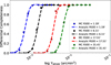 |
Fig. 3. Comparison of our MC completeness, averaged over the unmasked sky, to the semi-analytical ERF completeness for θ500 = 1.19′, 6.11′, 17.51′, and 31.41′, assuming an S/N threshold of 8.5. |
Following this validation, we extended our MC completeness calculation to triaxial clusters, constructing completeness curves to quantify how detection probability varies with triaxial axial ratios and orientation. In addition to the masks noted above, these samples included additional constraints: Tier 1 was limited to Dec > 0°, while both Tier 1 and Tier 2 had a low XMM-Newton visibility mask to exclude regions with visibilities < 55 ks per orbit (CHEX-MATE Collaboration 2021). From the unmasked sky regions, we again selected 100 widely separated map cutouts for both Tier 1 and Tier 2, ensuring good sampling of the available sky. We then inserted triaxial clusters with varying axial ratios, orientations, Y5R500, and θ500 into these cutouts and computed completeness by averaging detection probabilities over all sky positions. To model triaxial shape and orientation effects on MMF3 S/N, we introduced a new parameter,
 (12)
(12)
where, as before, llos is the semi-major axis of the ellipse along the LOS and (lp1 * lp2)0.5 is the effective spherical radius of the projected ellipse on the sky (see Fig. 2). We find that e′Δ exhibits a complex dependence on q1, q2, cos θ, and ϕ, but correlates monotonically with S/N–higher values of e′Δ correspond to higher S/N for a fixed (q1, q2), as shown in Fig. 4. We established this correlation for the full range of geometries considered in this paper, but we show only a subset in Fig. 4 for clarity. Thus, rather than using two separate orientation parameters (cos θ, ϕ), we consolidate them into e′Δ for each q1, q2. Using this framework, we constructed a comprehensive lookup table that quantifies detection probability as a function of SZ parameters and triaxial shape, thus describing P(d|Y500, θ500, q1, q2, e′Δ).
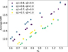 |
Fig. 4. Average MMF3 S/N as a function of e′Δ for different triaxial axial ratios, for a cluster with an effective spherical θ500 = 5.63′ and a fixed value of Y5R500. |
We present three slices of the five-parameter completeness function in Fig. 5, illustrating completeness as a function of triaxial axial ratios and orientations. We find a clear dependence on orientation, where clusters elongated along the LOS exhibit a higher probability of detection for the same Y5R500, θ500, and shape parameters. Additionally, we observe that for the same effective spherical θ500 but for other orientations, there is no clear trend between detectability and cluster triaxiality. We thus find that the primary factor influencing detectability is the extent of the cluster along the LOS. For triaxial clusters whose major axes are not closely aligned with the LOS, varying triaxialities can still result in more or less centrally peaked SZ profiles relative to spherical clusters, due to projection effects. Consistent with the results reported by Gallo et al. (2024), we find that the more centrally peaked clusters from this projection effect are more easily detected.
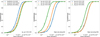 |
Fig. 5. Completeness as a function of Y5R500 for a cluster with effective spherical θ500 = 5.63′. Left: Completeness for different orientations of a cluster with q1 = 0.6, q2 = 0.8. Middle: Completeness for a cluster with different triaxialities, but with the major axis oriented along the LOS, with cos θ = 1.0, ϕ = 0°. Right: Completeness for a cluster with different triaxialities, but with the major axis oriented on the plane of sky (POS), with cos θ = 0.0, ϕ = 90°. |
To ensure a well-sampled and smoothly varying lookup table connecting detection probability with the relevant parameters, we fitted the completeness function for each (θ500, q1, q2, e′Δ) to an ERF of the form:
![Mathematical equation: $$ \begin{aligned} P(d) = \frac{1}{2}\left[1 + \mathrm{erf} \left(\frac{Y_{500} - q*a(R_{500}, q_1, q_2, e\prime _\Delta )}{\sqrt{2}*b(R_{500}, q_1, q_2, e\prime _\Delta )}\right)\right]. \end{aligned} $$](/articles/aa/full_html/2025/08/aa55719-25/aa55719-25-eq16.gif) (13)
(13)
Relative to the ERF in P16, this form incorporates modified mean (a) and variance (b) terms to capture non-Gaussian deviations introduced by cluster triaxiality. We then performed a grid interpolation over our lookup table to determine a and b as functions of q1, q2, and e′Δ.
5. Mock CHEXMATE catalogs
We used the triaxial completeness given by the ERF in Eq. (13) to construct mock CHEX-MATE catalogs, allowing us to quantify the average distribution of orientations and geometries that arise from this sample selection. First, we generated mock universes with halo populations sampled from the Tinker et al. (2008) HMF, assuming the Planck Collaboration VI (2020) cosmology, considering redshifts 0 ≤ z ≤ 0.6 and M500 masses between 1014 M⊙ and 1016 M⊙, while also applying the sky fraction constraints for both Tier 1 and Tier 2 samples. We converted the generated halo masses (M500) and redshifts (z) into θ500 and Y500 using the established scaling relations from Planck Collaboration XX (2014):
![Mathematical equation: $$ \begin{aligned} E^{-\beta }(z)\left[\frac{D_{\mathrm{A} }^2(z) \bar{Y}_{500}}{10^{-4}\,\mathrm{Mpc} ^2}\right] = Y_*\left[\frac{h}{0.7}\right]^{-2+\alpha }\left[\frac{(1-b) M_{500}}{6 \times 10^{14}\,\mathrm{M} _{\odot }}\right]^\alpha \end{aligned} $$](/articles/aa/full_html/2025/08/aa55719-25/aa55719-25-eq17.gif) (14)
(14)
and
![Mathematical equation: $$ \begin{aligned} \bar{\theta }_{500}=\theta _*\left[\frac{h}{0.7}\right]^{-2/3}\left[\frac{(1-b) M_{500}}{3 \times 10^{14}\,\mathrm{M}_{\odot }}\right]^{1/3} E^{-2/3}(z)\left[\frac{D_{\mathrm{A} }(z)}{500\,\mathrm{Mpc}}\right]^{-1}, \end{aligned} $$](/articles/aa/full_html/2025/08/aa55719-25/aa55719-25-eq18.gif) (15)
(15)
where E(z) = H(z)/H0, DA(z) is the angular diameter distance and (1 − b) is the mass bias factor, which is set to 0.62 for consistency with the cosmology obtained by Planck Collaboration VI (2020). The values of the scaling and normalization parameters were obtained from Planck Collaboration XXIV (2016). We then performed volume selections to form mock Tier 1 (0.05 < z < 0.2) and Tier 2 (z < 0.6) catalogs from halos generated using the HMF. To assign triaxial shapes and orientations to halos, we randomly draw axial ratio values for the gas from the empirical distributions obtained from the IllustrisTNG simulations presented in Machado Poletti Valle et al. (2021), along with random draws for cos θ ∈ [0, 1] and ϕ ∈ [0° ,90°]. Then, using the calibrated ERF, we computed the completeness for each halo and included it in the resulting catalog based on probabilistic sampling. Specifically, for each halo, we drew a uniform random value between 0 and 1, and included the halo in the catalog if the value of P(d) was larger than this random value. We repeated this process for 1000 mock universes for both Tier 1 and Tier 2.
Since Tier 2 requires an additional selection based on MMF3-derived mass, we reprocessed the completeness-selected clusters through the MMF3 algorithm. This provided the extracted Y500 for each cluster at every filter scale θ500 of MMF3. From this Y − θ relation we then determined the value of MMMF3 that simultaneously satisfied Eq. (14) and (15). Since this process was repeated across 100 distinct map cutouts, we obtained 100 different values of MMMF3 for each cluster, reflecting the variation in recovered mass due to noise fluctuations. To assign a single value of MMMF3 to each cluster, we performed a probabilistic selection based on the cluster’s detection completeness. Specifically, we randomly selected a value of MMMF3 from among the N highest values obtained from the 100 cutouts, where N = P(d)×100. This method effectively models the S/N-based mass boosting, as clusters with lower intrinsic S/N values are only included in the catalog when they fall within favorable map cutouts that result in boosted S/N values. Following CHEX-MATE, the final Tier 2 selection was then performed by requiring MMMF3 > 7.25 × 10¹⁴ M⊙.
As an additional validation of our detection pipeline, we find that the average number of halos detected across 1000 mock realizations for both the Tier 1 and Tier 2 selections is 59, closely matching the 61 clusters observed in the actual CHEX-MATE sample. Furthermore, as shown in Fig. 6, the mass and redshift distributions of the mock catalogs are consistent with the observed distributions when accounting for Poisson fluctuations due to the relatively small sample size. For Tier 1, the p-values from a KS test of the mass and redshift distributions are 0.43 and 0.29, indicating very good agreement. For Tier 2, the p-values are lower, equal to 0.011 for both the mass and redshift distributions, primarily due to the relative excess of high-mass and low-redshift systems detected in the mocks. While these p-values suggest possible discrepancies at low statistical significance, we note that Planck Collaboration XXIV (2016) also found a similar excess of low-z clusters predicted by the best-fit HMF relative to their abundance measurement from the Planck cluster catalog. We thus conclude that our Tier 2 mocks provide a reasonable description of the observed CHEX-MATE sample.
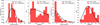 |
Fig. 6. Mass and redshift distributions for the observed Tier 1 and Tier 2 CHEX-MATE samples compared to the kernel density estimation (KDE) distribution of our 1000 mock CHEX-MATE selections. The distributions are consistent, indicating that the mock samples accurately reproduce the masses and redshifts of the observed samples. |
To assess the triaxial geometry of a CHEX-MATE-selected sample, Fig. 7 shows the distributions of cos θ and ϕ obtained for the Tier 1 and Tier 2 samples. For comparison, the values of cos θ and ϕ obtained from randomly selected halos matching the mass and redshift distributions of the CHEX-MATE-selected samples are also shown, and, as expected, are consistent with random orientations. Within the CHEX-MATE-selected samples, we see a clear excess in clusters that are elongated along the LOS, with a preference for halos with cos θ values close to 1 and ϕ values close to 0°, implying that an SZ selection results in a population biased toward LOS elongation. Quantitatively, the p-value obtained from a KS test comparing the distributions of e′Δ for the CHEX-MATE-selected and random samples is 2.7 × 10⁻³⁰, suggesting they are inconsistent at high statistical significance. We note that, while the excess of clusters with cos θ values near 1 is easy to understand, since it implies that the major axis is well aligned with the LOS, the excess of clusters with ϕ values close to 0° is more subtle. It arises because, when the major axis is well aligned with the POS (i.e., cos θ near 0), values of ϕ close to 0° imply that the intermediate axis is well aligned with the LOS. Thus, such clusters have a boosted SZ signal compared to those with ϕ close to 90°, which have their minor axis well aligned with the LOS.
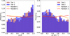 |
Fig. 7. Distributions of orientation angles cos θ and ϕ for the mock Tier 1 and Tier 2 samples, along with randomly selected samples with similar distributions in mass and redshift. The CHEX-MATE samples show a clear bias toward larger values of cos θ and smaller values of ϕ compared to the random samples, indicating that SZ selection favors clusters elongated along the LOS. |
6. Weak lensing mass bias
To assess whether the bias in orientation from an SZ selection results in a measurable MWL bias, we compared MWL estimates obtained from clusters detected in the mock CHEX-MATE catalogs to randomly selected samples of clusters with similar mass and redshift distributions. We generated mock shear maps for each mock cluster from its shape parameters, mass, and redshift, following Gavidia et al. (in prep.). In brief, we assumed that the gravitational potential follows the geometry of the ICM, which is described by a triaxial ellipsoid. Specifically, we adopted the same axial ratios and orientation for the gravitational potential as those used for the gas distribution when generating the mock SZ images. This assumption is well-motivated by simulations (e.g., Lau et al. 2011). An NFW density profile (Navarro et al. 1997) in a triaxial basis was used to model the cluster’s matter density distribution, and the gravitational potential was calculated via a numerical inversion of Poisson’s equation. The 3D gravitational potential was then projected to obtain the lensing potential, and partial derivatives of the model lensing potential were taken to obtain the model shear maps. As with the values of Y5R500 and θ500, the concentration c200 and total mass M200 (defined as MTrue hereafter) for these triaxial distributions were computed by spherically-averaging the 3D halo. For each halo, the values of the spherically-averaged c200 and MTrue were randomly drawn from the relation given by Diemer & Joyce (2019), assuming that log(c200) has an intrinsic scatter of 0.16. To isolate the impact of projection effects on these idealized mass estimates, we introduced a minimal level of uniform noise to the shear maps, approximately four orders of magnitude below current observational sensitivities.
These mock shear maps were then fitted to a spherically symmetric NFW model, analogous to the standard approachutilized for cosmological analyses, performed via a least-squares approach. Four different fits were performed using different values of c200, including fixing its value to either three or four, fixing its value based on the concentration-mass relation from Diemer & Joyce (2019), and allowing its value to float (within the range of one to ten). We performed these fits for the mock Tier 1 and Tier 2 samples, along with the randomly selected samples matching their redshift and mass distributions. We then computed the average ratio of the fitted MWL and the true halo mass, which we defined as 1 − bWL = MWL/MTrue, within discrete mass bins for all cases (see Fig. 8). For both Tier 1 and Tier 2, the MWL of the CHEX-MATE-selected samples is higher than that obtained from the random samples at the low-mass end, trending toward agreement at the high-mass end. This is as expected, since the up-scatter in S/N due to clusters elongated along LOS is more pronounced in lower-mass (and thus lower S/N) clusters, with higher-mass clusters generally having a higher S/N, which allows for detection irrespective of orientation. Furthermore, for c = 3 and c = 4, we see a sharp increase in MWL for both the random and CHEX-MATE-selected samples at the high-mass end. This is a result of utilizing the relation of Diemer & Joyce (2019) when generating the halos, as they find an increase in c200 at the high-mass end.
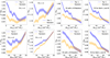 |
Fig. 8. Comparison of 1 − bWL as a function of true mass for the mock CHEX-MATE Tier 1 (top) and tier 2 (bottom) selected samples (purple lines and shaded 68% confidence level regions), compared to a random distribution of halos with matched mass and redshift distributions (orange lines and shaded 68% confidence level regions), using varying priors on the value of c200 to obtain MWL from the mock shear data. Left: c200 = 4. Middle left: c200 = 3. Middle right: c200 obtained from the c − M relation of Diemer & Joyce (2019). Right: c200 varied as a free parameter. |
We note that the overall value of 1 − bWL depends strongly on our fitting methodology, i.e., the assumed prior on c200, as expected due to the strong anti-correlation between c and M. However, the ratio of 1 − bWL obtained from the CHEX-MATE-selected and random samples, which we define as 1 − bχ, appears to be independent of the fitting methodology, as illustrated in Fig. 9. In other words, the portion of 1 − bWL associated with the on-average orientation of an SZ selection is robust to the choice of fitting method. For both Tier 1 and Tier 2, we find that 1 − bχ is approximately 4% at the low-mass end, with an overall average value near 2%. Thus, for the CHEX-MATE samples–and likely any Planck SZ-selected sample–the correction for this bias in 1 − bWL due to orientation should be universal, regardless of the WL fitting methodology. To facilitate such a correction, we provide the parameters of a linear regression fit of the form
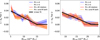 |
Fig. 9. Ratio of 1 − bWL forCHEX-MATE-selected samples (Left: Tier 1, Right: Tier 2), to 1 − bWL for random samples with matching mass and redshift distributions, defined as 1 − bχ. This plot isolates the bias due solely to orientation in an SZ-selected sample. This orientation bias is approximately independent of fitting methodology, as illustrated by the good agreement between all four choices used in this work. The black line shows a broken linear fit that reproduces the derived values of 1 − bχ to within an rms scatter of 0.003. |

to describe the selection-based orientation-induced bias in MWL for both the Tier 1 and Tier 2 samples, with the results summarized in Table 1. We find that these linear fits accurately reproduce the derived bias to within 0.3%, which is sufficient for percent-level mass calibration. Because of the different mass and redshift ranges for Tier 1 and Tier 2, along with the additional selection based on MMF3-derived mass for Tier 2, there is no expectation that the fitted slope and break point should be consistent between the two samples, and we indeed find modest differences in their values.
Parameters of the linear fit of 1 − bχ for the Tier 1 and Tier 2 CHEX-MATE samples, where 1 − bχ represents the bias in MWL due solely to orientation bias from the Planck SZ selection.
7. Conclusions
In this paper, we investigated the impact of triaxiality and orientation on SZ selection and the associated MWL values, focusing on the specific example of CHEX-MATE. Quantifying these selection effects is crucial for future cluster cosmology studies, as it enables corrections to the MWL values used for calibration of the halo masses.
To achieve this goal, we recreated the MMF3 algorithm used by P16 for the detection of clusters based on their SZ signal in the Planck all-sky maps. Using an MC method based on the injection of mock clusters into randomly sampled cutouts from Planck HFI maps within the unmasked region of the sky, we confirm that the values of S/N and Y5R500 obtained from our implementation of the MMF3 are consistent with those obtained by P16 for spherically-symmetric clusters. By then applying this algorithm to mock observations of clusters with triaxial shapes, we determined the completeness as a function of SZ signal strength, angular size, and triaxial shape and orientation.
Using our measured triaxial completeness, we constructed mock CHEX-MATE catalogs to quantify selection biases introduced by triaxiality and orientation for SZ-detected clusters. We find a clear orientation bias, where clusters elongated along the LOS are preferentially detected due to their centrally boosted SZ signals. By fitting MWL to the mock Tier 1 and Tier 2 detected clusters, along with randomly selected clusters with comparable mass and redshift distributions, we identify a mass-dependent MWL bias due solely to the shape and orientation of the SZ-selected samples, 1 − bχ. This bias reaches up to 4% in the lowest-mass clusters and averages approximately 2% across the full mass range. In addition, 1 − bχ appears to be independent of the exact WL fitting methodology. We also note that the value of 1 − bχ found here is expected to be a lower limit, since we do not account for correlated LSS in our selection or WL modeling. Such structures are expected to occur preferentially along the halo elongation direction, and would thus boost the SZ signal when viewed in that orientation, resulting in a stronger preference for LOS elongation in the CHEX-MATE-selected samples, as well as boosting the value of MWL at fixed LOS elongation.
We also consider the implications of our results in the context of cluster cosmology from halo abundance measurements. First, we find that MWL is systematically overestimated in SZ-selected samples from Planck, implying that true masses are, on average, lower than WL-derived masses for such samples. The discrepancy between halo abundance and primary CMB measurements from Planck requires higher halo masses for the cluster sample, so this correction acts in the opposite direction. In addition, we note that the average 2% systematic overestimate of MWL measured here is subdominant to current systematic uncertainties in MWL calibration. Thus it does not significantly impact previously published results. However, upcoming surveys like CMB-S4 and Euclid require percent-level mass calibration (Raghunathan et al. 2022; Euclid Collaboration: Giocoli et al. 2024; Euclid Collaboration: Ragagnin et al. 2025), and therefore such biases must be accounted for in their analyses.
R500 denotes the spherical radius enclosing an average overdensity 500 times larger than the critical density of the Universe at the cluster redshift.
Acknowledgments
This research was supported by the International Space Science Institute (ISSI) in Bern, through ISSI International Team project #565 (Multi-Wavelength Studies of the Culmination of Structure Formation in the Universe). H.S., J.S., A.G. and J.K. were supported by NASA Astrophysics Data Analysis Program (ADAP) Grant 80NSSC21K1571. SE, MS, MR acknowledges the financial contribution from the contracts Prin-MUR 2022 supported by Next Generation EU (M4.C2.1.1, n.20227RNLY3 The concordance cosmological model: stress-tests with galaxy clusters). MS acknowledges the financial contributions from contract INAF mainstream project 1.05.01.86.10 and INAF Theory Grant 2023: Gravitational lensing detection of matter distribution at galaxy cluster boundaries and beyond (1.05.23.06.17). SE, MR acknowledges the financial contributions from the European Union’s Horizon 2020 Programme under the AHEAD2020 project (grant agreement n. 871158). GWP acknowledges long-term support from CNES, the French space agency. LL acknowledges the financial contribution from the INAF grant 1.05.12.04.01. EP acknowledges support from CNES, the French national space agency and from ANR the French Agence Nationale de la Recherche, under grant ANR-22-CE31-0010. J.K. acknowledges the support by Basic Science Research Program through the National Research Foundation of Korea (NRF) funded by the Ministry of Education(2019R1A6A1A10073887) and the 2025 KAIST-U.S. Joint Research Collaboration Open Track Project for Early-Career Researchers, supported by the International Office at the Korea Advanced Institute of Science and Technology (KAIST). M.G. acknowledges support from the ERC Consolidator Grant BlackHoleWeather (101086804). MDP acknowledges financial support from PRIN-MUR grant 20228B938N “Mass and selection biases of galaxy clusters: a multi-probe approach” funded by the European Union Next generation EU, Mission 4 Component 1 CUP C53D2300092 0006. DE acknowledges support from the Swiss National Science Foundation (SNSF) through grant agreement #200021_212576. BJM acknowledges support from Science and Technology Facilities Council grants ST/V000454/1 and ST/Y002008/1.
References
- Abbott, T. M. C., Aguena, M., Alarcon, A., et al. 2020, Phys. Rev. D, 102, 023509 [Google Scholar]
- Allen, S. W., Evrard, A. E., & Mantz, A. B. 2011, ARA&A, 49, 409 [Google Scholar]
- Arnaud, M., Pratt, G. W., Piffaretti, R., et al. 2010, A&A, 517, A92 [CrossRef] [EDP Sciences] [Google Scholar]
- Becker, M. R., & Kravtsov, A. V. 2011, ApJ, 740, 25 [NASA ADS] [CrossRef] [Google Scholar]
- Bellagamba, F., Roncarelli, M., Maturi, M., & Moscardini, L. 2017, MNRAS, 473, 5221 [Google Scholar]
- Bleem, L. E., Stalder, B., de Haan, T., et al. 2015, ApJS, 216, 27 [Google Scholar]
- Bleem, L. E., Klein, M., Abbot, T. M. C., et al. 2024, Open J. Astrophys., 7, 13 [CrossRef] [Google Scholar]
- Bocquet, S., Grandis, S., Bleem, L. E., et al. 2024, Phys. Rev. D, 110, 083510 [NASA ADS] [CrossRef] [Google Scholar]
- Bonamigo, M., Despali, G., Limousin, M., et al. 2015, MNRAS, 449, 3171 [NASA ADS] [CrossRef] [Google Scholar]
- CHEX-MATE Collaboration (Arnaud, M., et al.) 2021, A&A, 650, A104 [NASA ADS] [CrossRef] [EDP Sciences] [Google Scholar]
- Chiu, I. N., Ghirardini, V., Liu, A., et al. 2022, A&A, 661, A11 [NASA ADS] [CrossRef] [EDP Sciences] [Google Scholar]
- Costanzi, M., Rozo, E., Simet, M., et al. 2019, MNRAS, 488, 4779 [NASA ADS] [CrossRef] [Google Scholar]
- Costanzi, M., Saro, A., Bocquet, S., et al. 2021, Phys. Rev. D, 103, 043522 [Google Scholar]
- DES Collaboration (Abbott, T. M. C.) 2025, ArXiv e-prints [arXiv:2503.13632] [Google Scholar]
- Despali, G., Giocoli, C., & Tormen, G. 2014, MNRAS, 443, 3208 [Google Scholar]
- Despali, G., Giocoli, C., Angulo, R. E., et al. 2016, MNRAS, 456, 2486 [NASA ADS] [CrossRef] [Google Scholar]
- Diemer, B., & Joyce, M. 2019, ApJ, 871, 168 [NASA ADS] [CrossRef] [Google Scholar]
- Euclid Collaboration (Giocoli, C., et al.) 2024, A&A, 681, A67 [NASA ADS] [CrossRef] [EDP Sciences] [Google Scholar]
- Euclid Collaboration (Ragagnin, A., et al.) 2025, A&A, 695, A282 [Google Scholar]
- Gallo, S., Douspis, M., Soubrié, E., & Salvati, L. 2024, A&A, 686, A15 [NASA ADS] [CrossRef] [EDP Sciences] [Google Scholar]
- Ghirardini, V., Bulbul, E., Artis, E., et al. 2024, A&A, 689, A298 [NASA ADS] [CrossRef] [EDP Sciences] [Google Scholar]
- Giocoli, C., Despali, G., Meneghetti, M., et al. 2025, A&A, 697, A184 [NASA ADS] [CrossRef] [EDP Sciences] [Google Scholar]
- Grandis, S., Ghirardini, V., Bocquet, S., et al. 2024, A&A, 687, A178 [NASA ADS] [CrossRef] [EDP Sciences] [Google Scholar]
- Hilton, M., Sifón, C., Naess, S., et al. 2021, ApJS, 253, 3 [Google Scholar]
- Hoekstra, H., Herbonnet, R., Muzzin, A., et al. 2015, MNRAS, 449, 685 [NASA ADS] [CrossRef] [Google Scholar]
- Kim, J., Sayers, J., Sereno, M., et al. 2024, A&A, 686, A97 [NASA ADS] [CrossRef] [EDP Sciences] [Google Scholar]
- Kleinebreil, F., Grandis, S., Schrabback, T., et al. 2025, A&A, 695, A216 [NASA ADS] [CrossRef] [EDP Sciences] [Google Scholar]
- Kornoelje, K., Bleem, L. E., Rykoff, E. S., et al. 2025, ApJ, submitted [arXiv:2503.17271] [Google Scholar]
- Lau, E. T., Nagai, D., Kravtsov, A. V., & Zentner, A. R. 2011, ApJ, 734, 93 [CrossRef] [Google Scholar]
- Lau, E. T., Nagai, D., Kravtsov, A. V., Vikhlinin, A., & Zentner, A. R. 2012, ApJ, 755, 116 [NASA ADS] [CrossRef] [Google Scholar]
- Lesci, G. F., Marulli, F., Moscardini, L., et al. 2022a, A&A, 659, A88 [NASA ADS] [CrossRef] [EDP Sciences] [Google Scholar]
- Lesci, G. F., Nanni, L., Marulli, F., et al. 2022b, A&A, 665, A100 [NASA ADS] [CrossRef] [EDP Sciences] [Google Scholar]
- Limousin, M., Morandi, A., Sereno, M., et al. 2013, Space Sci. Rev., 177, 155 [Google Scholar]
- Machado Poletti Valle, L. F., Avestruz, C., Barnes, D. J., et al. 2021, MNRAS, 507, 1468 [CrossRef] [Google Scholar]
- Mantz, A., Allen, S. W., Rapetti, D., & Ebeling, H. 2010, MNRAS, 406, 1759 [NASA ADS] [Google Scholar]
- Mantz, A. B., von der Linden, A., Allen, S. W., et al. 2015, MNRAS, 446, 2205 [Google Scholar]
- Melin, J.-B., Bartlett, J. G., & Delabrouille, J. 2006, A&A, 459, 341 [NASA ADS] [CrossRef] [EDP Sciences] [Google Scholar]
- Melin, J. B., Aghanim, N., Bartelmann, M., et al. 2012, A&A, 548, A51 [NASA ADS] [CrossRef] [EDP Sciences] [Google Scholar]
- Meneghetti, M., Rasia, E., Merten, J., et al. 2010, A&A, 514, A93 [NASA ADS] [CrossRef] [EDP Sciences] [Google Scholar]
- Nagai, D., Kravtsov, A. V., & Vikhlinin, A. 2007, ApJ, 668, 1 [Google Scholar]
- Navarro, J. F., Frenk, C. S., & White, S. D. M. 1997, ApJ, 490, 493 [Google Scholar]
- Oguri, M., Bayliss, M. B., Dahle, H., et al. 2012, MNRAS, 420, 3213 [Google Scholar]
- Okabe, N., Reiprich, T. H., Grandis, S., et al. 2025, A&A, 700, A46 [NASA ADS] [CrossRef] [EDP Sciences] [Google Scholar]
- Pacaud, F., Pierre, M., Melin, J.-B., et al. 2018, A&A, 620, A10 [NASA ADS] [CrossRef] [EDP Sciences] [Google Scholar]
- Planck Collaboration XX. 2014, A&A, 571, A20 [NASA ADS] [CrossRef] [EDP Sciences] [Google Scholar]
- Planck Collaboration XI. 2016, A&A, 594, A11 [NASA ADS] [CrossRef] [EDP Sciences] [Google Scholar]
- Planck Collaboration XXIV. 2016, A&A, 594, A24 [NASA ADS] [CrossRef] [EDP Sciences] [Google Scholar]
- Planck Collaboration XXVI. 2016, A&A, 594, A26 [NASA ADS] [CrossRef] [EDP Sciences] [Google Scholar]
- Planck Collaboration XXVII. 2016, A&A, 594, A27 [NASA ADS] [CrossRef] [EDP Sciences] [Google Scholar]
- Planck Collaboration VI. 2020, A&A, 641, A6 [NASA ADS] [CrossRef] [EDP Sciences] [Google Scholar]
- Pratt, G. W., Arnaud, M., Biviano, A., et al. 2019, Space Sci. Rev., 215, 25 [Google Scholar]
- Raghunathan, S., Whitehorn, N., Alvarez, M. A., et al. 2022, ApJ, 926, 172 [NASA ADS] [CrossRef] [Google Scholar]
- Rozo, E., Wechsler, R. H., Rykoff, E. S., et al. 2010, ApJ, 708, 645 [Google Scholar]
- Rykoff, E. S., Rozo, E., Busha, M. T., et al. 2014, ApJ, 785, 104 [Google Scholar]
- Sarazin, C. L. 1986, Rev. Mod. Phys., 58, 1 [Google Scholar]
- Sayers, J., Golwala, S. R., Ameglio, S., & Pierpaoli, E. 2011, ApJ, 728, 39 [NASA ADS] [CrossRef] [Google Scholar]
- Sehgal, N., Trac, H., Acquaviva, V., et al. 2011, ApJ, 732, 44 [NASA ADS] [CrossRef] [Google Scholar]
- Sereno, M., Umetsu, K., Ettori, S., et al. 2018, ApJ, 860, L4 [NASA ADS] [CrossRef] [Google Scholar]
- Sunyaev, R. A., & Zeldovich, Y. B. 1972, Comments Astrophys. Space Phys., 4, 173 [NASA ADS] [EDP Sciences] [Google Scholar]
- Tinker, J., Kravtsov, A. V., Klypin, A., et al. 2008, ApJ, 688, 709 [Google Scholar]
- To, C., Krause, E., Rozo, E., et al. 2021, Phys. Rev. Lett., 126, 141301 [NASA ADS] [CrossRef] [Google Scholar]
- Vega-Ferrero, J., Yepes, G., & Gottlöber, S. 2017, MNRAS, 467, 3226 [Google Scholar]
- Vikhlinin, A., Kravtsov, A. V., Burenin, R. A., et al. 2009, ApJ, 692, 1060 [Google Scholar]
- Voit, G. M. 2005, Rev. Mod. Phys., 77, 207 [Google Scholar]
- von der Linden, A., Mantz, A., Allen, S. W., et al. 2014, MNRAS, 443, 1973 [NASA ADS] [CrossRef] [Google Scholar]
All Tables
Parameters of the linear fit of 1 − bχ for the Tier 1 and Tier 2 CHEX-MATE samples, where 1 − bχ represents the bias in MWL due solely to orientation bias from the Planck SZ selection.
All Figures
|
Fig. 1. Histogram of the difference in S/N obtained from our implementation of the MMF3 detection algorithm and that used by P16 for the CHEX-MATE clusters. |
| In the text | |
|
Fig. 2. Triaxial ellipsoid model used in the analysis. The intrinsic coordinate system of the ellipsoid is indicated by the dotted arrows, and the black arrows correspond to the observer’s coordinate system. The red ellipse shows the projection of the ellipsoid on the sky plane, with lp1 as its semi-major axis. The green ellipse shows the projection of the ellipsoid onto the plane perpendicular to the sky plane, and llos is the half size of the ellipse along the observer line of sight (Kim et al. 2024). |
| In the text | |
|
Fig. 3. Comparison of our MC completeness, averaged over the unmasked sky, to the semi-analytical ERF completeness for θ500 = 1.19′, 6.11′, 17.51′, and 31.41′, assuming an S/N threshold of 8.5. |
| In the text | |
|
Fig. 4. Average MMF3 S/N as a function of e′Δ for different triaxial axial ratios, for a cluster with an effective spherical θ500 = 5.63′ and a fixed value of Y5R500. |
| In the text | |
|
Fig. 5. Completeness as a function of Y5R500 for a cluster with effective spherical θ500 = 5.63′. Left: Completeness for different orientations of a cluster with q1 = 0.6, q2 = 0.8. Middle: Completeness for a cluster with different triaxialities, but with the major axis oriented along the LOS, with cos θ = 1.0, ϕ = 0°. Right: Completeness for a cluster with different triaxialities, but with the major axis oriented on the plane of sky (POS), with cos θ = 0.0, ϕ = 90°. |
| In the text | |
|
Fig. 6. Mass and redshift distributions for the observed Tier 1 and Tier 2 CHEX-MATE samples compared to the kernel density estimation (KDE) distribution of our 1000 mock CHEX-MATE selections. The distributions are consistent, indicating that the mock samples accurately reproduce the masses and redshifts of the observed samples. |
| In the text | |
|
Fig. 7. Distributions of orientation angles cos θ and ϕ for the mock Tier 1 and Tier 2 samples, along with randomly selected samples with similar distributions in mass and redshift. The CHEX-MATE samples show a clear bias toward larger values of cos θ and smaller values of ϕ compared to the random samples, indicating that SZ selection favors clusters elongated along the LOS. |
| In the text | |
|
Fig. 8. Comparison of 1 − bWL as a function of true mass for the mock CHEX-MATE Tier 1 (top) and tier 2 (bottom) selected samples (purple lines and shaded 68% confidence level regions), compared to a random distribution of halos with matched mass and redshift distributions (orange lines and shaded 68% confidence level regions), using varying priors on the value of c200 to obtain MWL from the mock shear data. Left: c200 = 4. Middle left: c200 = 3. Middle right: c200 obtained from the c − M relation of Diemer & Joyce (2019). Right: c200 varied as a free parameter. |
| In the text | |
|
Fig. 9. Ratio of 1 − bWL forCHEX-MATE-selected samples (Left: Tier 1, Right: Tier 2), to 1 − bWL for random samples with matching mass and redshift distributions, defined as 1 − bχ. This plot isolates the bias due solely to orientation in an SZ-selected sample. This orientation bias is approximately independent of fitting methodology, as illustrated by the good agreement between all four choices used in this work. The black line shows a broken linear fit that reproduces the derived values of 1 − bχ to within an rms scatter of 0.003. |
| In the text | |
Current usage metrics show cumulative count of Article Views (full-text article views including HTML views, PDF and ePub downloads, according to the available data) and Abstracts Views on Vision4Press platform.
Data correspond to usage on the plateform after 2015. The current usage metrics is available 48-96 hours after online publication and is updated daily on week days.
Initial download of the metrics may take a while.