| Issue |
A&A
Volume 700, August 2025
|
|
|---|---|---|
| Article Number | L16 | |
| Number of page(s) | 6 | |
| Section | Letters to the Editor | |
| DOI | https://doi.org/10.1051/0004-6361/202555937 | |
| Published online | 15 August 2025 | |
Letter to the Editor
An analytic formalism to describe the Neff(H)−nH relationship in molecular clouds
Faculty of Physics, University of Duisburg-Essen, Lotharstraße 1, 47057 Duisburg, Germany
⋆ Corresponding author: This email address is being protected from spambots. You need JavaScript enabled to view it.
Received:
13
June
2025
Accepted:
22
July
2025
Abstract
Context. Astrochemical modeling requires, as input, the effective column density of gas (or extinction) that attenuates an external, isotropic, far-ultraviolet radiation field. In three-dimensional simulations, this can be calculated through ray-tracing schemes, while in zero-dimensional chemical models it is often treated as a free parameter.
Aims. We aim to produce an analytic, physically motivated formalism to predict the average relationship between the effective hydrogen-nucleus column density, Neff(H), and the local hydrogen-nucleus number density, nH.
Methods. We constructed an analytic model utilizing characteristic length scales that connects the turbulence-dominated regime and the gravitational-dominated regime at high densities.
Results. The model reproduces a previous analytic fit to simulation results well and is consistent with the high-density power-law indices, for example Neff(H)∝nγ, where γ ≈ 0.4 − 0.5, found in previous numerical simulations utilizing ray-tracing.
Conclusions. We present an analytic model that relates the average effective column density, Neff, to the local number density, nH, and reproduces the behaviors found in three-dimensional simulations. The analytic model can be utilized as a sub-grid prescription for shielded molecular gas or in astrochemical models for a physically motivated estimation of the attenuating column density.
Key words: ISM: clouds / ISM: general / ISM: structure
© The Authors 2025
 Open Access article, published by EDP Sciences, under the terms of the Creative Commons Attribution License (https://creativecommons.org/licenses/by/4.0), which permits unrestricted use, distribution, and reproduction in any medium, provided the original work is properly cited.
This article is published in open access under the Subscribe to Open model. This email address is being protected from spambots. You need JavaScript enabled to view it. to support open access publication.
1. Introduction
The chemistry of the molecular clouds plays a vital role in our understanding of the star formation process. Observationally, the dynamics of molecular clouds are constrained through the Doppler shift of molecular line emission. Chemistry also plays an important role in the thermodynamics of molecular clouds through atomic and molecular line cooling (Draine 2011; Tielens 2013). Therefore, astrochemical models of molecular clouds are central in both theoretical and observational studies of star formation and the physics of molecular clouds.
In astrochemical modeling, the effective attenuating column density for the external radiation field is a primary input (Wakelam et al. 2013; Bovino & Grassi 2024). This effective column density, Neff (the column density of hydrogen nuclei), or the effective extinction, AV, eff (magnitude), gives the local far-ultraviolet (FUV) flux, χ/χ0 ∝ e−AV, eff, where χ0 is the FUV flux at the cloud boundary. In the case of isotropic radiation, the effective column density at a point, x, is the weighted average (see below) of all directions of the integrated column density from point x to the cloud boundary. It is thus different from the observational column density, which is integrated through the entire cloud along an observed line of sight. Given the importance of this parameter to astrochemical models, estimating it is crucial for accurate chemical models of molecular clouds.
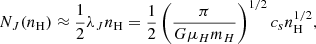
Astrochemical models have to make a choice for Neff, such as assuming it is equal to the observed column density or leaving it as a free parameter in model fitting. In molecular cloud simulations, Neff is often calculated through ray-tracing (e.g., Nelson & Langer 1997; Glover & Mac Low 2007; Glover et al. 2010; Van Loo et al. 2013; Safranek-Shrader et al. 2017; Seifried et al. 2017; Hu et al. 2021; Wünsch 2024), where the hydrogen nucleus column density is summed along each ray out of the domain from each cell using, for example, a HEALPIX-based method for the ray directions, or the simpler six-ray approach along each cardinal direction. The effective extinction is the average,
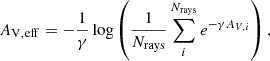 (1)
(1)
where the coefficient, γ, is a normalization constant chosen to be the photo-destruction rate coefficient for particular molecules (e.g., Glover et al. 2010; Hu et al. 2021) or is based on dust absorption (e.g., Nelson & Langer 1997). When no ray-tracing is used, Neff is computed using an assumed physical length scale and the cell’s density (see the discussion in Safranek-Shrader et al. 2017). Recently, Bisbas et al. (2023, hereafter B23) provided a fit to several hydrodynamic simulations for AV, eff − nH,
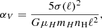
![Mathematical equation: $$ \begin{aligned} A_{\rm V, eff} = 0.05 \exp \left[1.6\, \left( \frac{n_{\rm H}}{\mathrm{cm}^{-3}} \right)^{0.12} \right]. \end{aligned} $$](/articles/aa/full_html/2025/08/aa55937-25/aa55937-25-eq2.gif) (2)
(2)
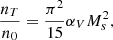
However, this fit is biased by the assumptions and initial conditions in the underlying simulations: the simulations were predominantly for Milky Way-like clouds, with both a resolution limit and a numerical column density floor. Safranek-Shrader et al. (2017) and Hu et al. (2021) also fitted a polynomial from their simulations and for nH > 10 cm−3 found  .
.
In this Letter we present a simple analytic model connecting the local gas density to the effective column density. The model is derived such that, with few assumptions about the cloud-scale turbulence and dynamics, an effective column density can be estimated that is in general agreement with the results from three-dimensional simulations. In Sect. 2 we present the underlying model components. In Sect. 3 we show the results of the model in comparison to the previous three-dimensional calculations. Finally, in Sect. 4 we discuss the potential applications for this model and its limitations, and provide some concluding remarks.
2. Methods
We built an analytic model to reproduce a characteristic Neff(H)−nH relationship from a simple, physically intuitive construction. We built up the model by considering three different characteristic length scales: (i) turbulent, (ii) gravitational, and (iii) numerical resolution. Figure 1 shows a chart of the scales of interest and the various parameters that enter into the model.
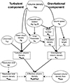 |
Fig. 1. Chart showing the different components and where parameters enter into the model. |
2.1. Turbulence length scale
Within the molecular cloud, any particular parcel of gas is surrounded by an envelope of turbulent gas that attenuates the external FUV radiation. We assumed this column density is, on average, related to an effective length scale, ℓturb, outwards to the cloud boundary through the turbulent envelope multiplied by the average number density, n0, in the turbulent envelope,
 (3)
(3)
If the cloud depth is known, for example from three-dimensional cloud maps that use observations from Gaia (Zucker et al. 2021; Rezaei Kh. et al. 2024; Edenhofer et al. 2024), and there is a measured column density distribution function, this can be estimated by dividing the mean of the log-normal component by the cloud depth.
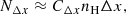
We assumed that at a given number density, nH, we can determine a characteristic length scale ℓ, given assumptions on the macroscopic cloud properties. We utilized the virial parameter, αV, to calculate this effective size as a function of density, defined by
 (4)
(4)
where σ(ℓ) is the turbulence velocity dispersion as a function of the length scale, G is the gravitational constant, μH is the mean molecular weight per hydrogen nucleus, and mH is the mass of hydrogen. To get the above expression, we have assumed that the mass and density are connected via M ≈ ρℓ3. Relating a length scale to the density and virial parameter assumes a hierarchical density structure. The linewidth-size relationship is
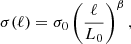 (5)
(5)
where σ0 and L0 are the normalization velocity and scale (or driving scale), respectively, and β is related to the physics behind the turbulence cascade (Larson 1981; Heyer & Dame 2015). Recent surveys have shown that β typically ranges between 0.3 and 0.67 (Rice et al. 2016; Kauffmann et al. 2017; Spilker et al. 2022). Combining Eqs. (4) and (5) gives us the length scale,
![Mathematical equation: $$ \begin{aligned} \ell = \left[ \frac{G L_0^{2\beta }\mu _H m_H n_{\rm H}}{5\sigma _0^2} \alpha _v\right]^{1/[2(\beta -1)]}. \end{aligned} $$](/articles/aa/full_html/2025/08/aa55937-25/aa55937-25-eq7.gif) (6)
(6)
At low densities or high virial parameters, this length scale, ℓ, can exceed the cloud size, Lcl. Therefore, we computed a modified length to limit ℓ to be less than Lcl,
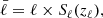 (7)
(7)
where zℓ = Lcl/ℓ. The dampening function requires that for ℓ < < Lcl,  , and for ℓ ≳ Lcl,
  . We adopted
 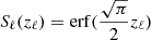 since it closely approximates a step-function filter while remaining smooth at all scales. This choice primarily impacts the lowest densities. The length scale out of the cloud is then
 (8)
(8)
where  is the cloud radius. In low-density gas, more likely to be in the outer regions, ℓturb → 0, and so Nturb → 0. Conversely, in the dense gas, ℓturb → Rcl, and so Nturb → n0Rcl. Since the effective column density for an isotropic external radiation field is most sensitive to the lowest column density to the cloud boundary, it can be readily seen for any approximately spherically symmetric cloud that the maximum ℓturb is Rcl.
2.2. Gravitational length scale
In the high-density limit, the effective column density is dominated by gravitationally bound gas in the immediate surroundings. The length scale of relevance here is the Jeans length, λJ. We defined this component as
 (9)
(9)
where 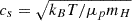 is the sound speed, T is the gas temperature, kB is the Boltzmann constant, and μp is the mean molecular mass per free particle. Under isothermal conditions,
  .
.
We accounted for the fact that gravity is not dominant at all densities by introducing a threshold that determines when gravity becomes dynamically important. We denote the threshold function as Sn(nH/nT), where nT is the transition density. A good parameterization of nT equates the Jeans length and turbulence sonic scale, and following Burkhart & Mocz (2019) for isothermal turbulence,
 (10)
(10)
where Ms and αV are calculated at L0 using σ0, which is similar to the expression in Padoan & Nordlund (2011).
We adopted a softened threshold, Sn(zn) = zn/(1 + zn), where zn = nH/nT. The choice of threshold impacts how rapidly or slowly the effective column density transitions between the turbulence- and gravity-dominated regimes. The total gravitational column density is
 (11)
(11)
2.3. Resolution limits
In hydrodynamic simulations, the total attenuating column is constrained by the limited resolution (Glover et al. 2010; Van Loo et al. 2013). The resolution limit imposes a floor for the attenuation column density,
 (12)
(12)
where the prefactor CΔx depends on how the self-contribution is accounted for, for example a whole cell size or half a cell size.
2.4. Combined model
The final Neff(H)−nH relation without numerical resolution effects is
 (13)
(13)
If a restriction based on resolution is needed, then the expression is modified to
 (14)
(14)
To enable comparisons with B23, we also used a floor of 0.05 mag.
3. Results
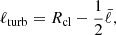
For our fiducial model, we aim to model Milky Way-like molecular clouds. We adopted the fiducial parameters in Table 1, mean molecular weights, μH = 1.4 and μp = 2.33, a conversion factor between the hydrogen nucleus column density and visual extinction of AV = 6.29 × 10⁻²²N(H) (Röllig et al. 2007), and a normalization scale for the linewidth-size relationship of L0 = 1 pc. In Appendix A we investigate the impact of assuming a fixed cs and μp and show that assumptions on μp have a minimal impact, while a variable cs can increase Neff at intermediate and low densities. However, these have less of an impact than varying key physical parameters.
Important physical parameters.
Figure 2 shows the fiducial model in comparison to the B23 fit. At moderate densities, the model matches B23 within a factor of two, although toward low densities, a floor is needed to remain consistent with B23. The slope flattens around nH ≈ 500 cm−3 due to the transition between the turbulent to gravitational components. At high densities, Neff is dominated by the gravitational component with a slope flatter than 0.5 due to the contribution of the turbulent column, even with an isothermal assumption. The fiducial model slope between 103 ≤ nH ≤ 105 is consistent with the  and
and  found in the simulations of Safranek-Shrader et al. (2017) and Hu et al. (2021), respectively. The inclusion of the relevant resolution limit and floor brings the model into excellent agreement with that of B23.
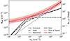 |
Fig. 2. Fiducial model results for the Neff(H)−nH relationship. The different components and totals are annotated. The red line shows the Bisbas et al. (2023) fit, and the band shows a factor of 2 deviation from it. The secondary y-axis shows the extinction using a scalar conversion factor as described in the text. “Total w/ biases” includes the resolution limit and floor. |
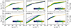 |
Fig. 3. Parameter space results for the Neff(H)−nH relationship. In each panel the annotated parameter is varied but the others are fixed to the fiducial values given in Table 1. |
We also investigated the impact of varying the major underlying parameters given in Table 1. Figure 3 shows the impact of varying six different parameters on the Neff(H)−nH relationship. For the parameter study, we only varied one parameter at a time, keeping the rest fixed at the fiducial value. At high densities, the only parameters that have a noticeable impact are the gas temperature, which increases the Jeans radius, and the average ambient turbulent density, which globally shifts the attenuating column.
As expected, increasing the cloud size or the average turbulent density increases the turbulent column and causes the slope to flatten around n(H)≈103 cm−3. Further, decreasing the strength of the turbulence or the linewidth-size slope increases the turbulent column density. For isotropic hydrodynamic turbulence, the Neff(H)−nH relationship maintains a relatively constant slope at all densities, consistent with the Neff ∝ n0.42 found in the hydrodynamic simulations of Safranek-Shrader et al. (2017). The virial parameter does not have a significant impact on the results, since it impacts ℓ and nT in opposite directions. In Appendix B we detail the calculation of the slopes of the Neff(H)−nH function, compare them to the fitted power-law slopes, and show that toward high densities the model is in good agreement with simulations.
4. Discussion and conclusions
An analytic expression for the Neff(H)−nH relationship is advantageous for both simulations and chemical models of molecular clouds. Astrochemical codes, in particular zero-dimensional models, rely on the input of a meaningful attenuating column density along with the density, temperature, and surface FUV radiation field. Further, the Neff(H)−nH relationship can be used to generate a one-dimensional density distribution for rapid one-dimensional photodissociation region models (see, e.g., Bisbas et al. 2021, 2023). For observations of unresolved molecular clouds, the use of Neff(H)−nH one-dimensional photodissociation region models can be used with the input physical parameters to gain insights into the physics of the cloud.
In hydrodynamic simulations that model molecular clouds, performing radiative transfer can be cost-prohibitive. In such instances, this analytic model can be utilized as a sub-grid model to rapidly estimate the attenuating column density. While this will not replicate the accuracy of a full radiative transfer simulation, it is worth highlighting that even in such simulations, the spread in Av as a function of density decreases with increasing density (see e.g. Hu et al. 2021); therefore, toward higher densities, the impact of using this model versus full ray-tracing is reduced. Finally, attenuating column densities are not just used for FUV radiation, but also for cosmic-ray energy losses into clouds (see, e.g., Padovani et al. 2009; Gaches et al. 2022).
In this Letter we have presented an analytic model for estimating the effective column density, Neff, which acts as the attenuating column density of an isotropic external radiation field, as a function of the local hydrogen-nucleus number density, nH. We have demonstrated that our fiducial model, which aims to represent clouds similar to those of the solar neighborhood, qualitatively reproduces the function presented by B23, which is a fit to several three-dimensional simulations with radiative transfer, and the power-law behavior toward high densities found in other works, such as Glover et al. (2010), Van Loo et al. (2013), Safranek-Shrader et al. (2017), and Hu et al. (2021). The analytic model can enable the rapid estimation of effective column densities for astrochemical models and act as a sub-grid model in simulations of molecular clouds that do not include radiative transfer. Future work will combine this model into grids of photodissociation region codes to estimate macroscopic cloud parameters from molecular line observations.
Acknowledgments
We thank the anonymous referee for their useful suggestions, which improved this Letter, and Thomas Bisbas and Daniel Seifried for their thoughtful discussions. BALG is supported by the German Research Foundation (DFG) in the form of an Emmy Noether Research Group - DFG project #542802847 (GA 3170/3-1).
References
- Bisbas, T. G., Bell, T. A., Viti, S., Yates, J., & Barlow, M. J. 2012, MNRAS, 427, 2100 [NASA ADS] [CrossRef] [Google Scholar]
- Bisbas, T. G., Tan, J. C., & Tanaka, K. E. I. 2021, MNRAS, 502, 2701 [CrossRef] [Google Scholar]
- Bisbas, T. G., van Dishoeck, E. F., Hu, C.-Y., & Schruba, A. 2023, MNRAS, 519, 729 [Google Scholar]
- Bovino, S., & Grassi, T. 2024, Astrochemical Modeling: Practical Aspects of Microphysics in Numerical Simulations (Elsevier) [Google Scholar]
- Burkhart, B., & Mocz, P. 2019, ApJ, 879, 129 [NASA ADS] [CrossRef] [Google Scholar]
- Draine, B. T. 1978, ApJS, 36, 595 [Google Scholar]
- Draine, B. T. 2011, Physics of the Interstellar and Intergalactic Medium (Princeton University Press) [Google Scholar]
- Edenhofer, G., Zucker, C., Frank, P., et al. 2024, A&A, 685, A82 [NASA ADS] [CrossRef] [EDP Sciences] [Google Scholar]
- Gaches, B. A. L., Bisbas, T. G., & Bialy, S. 2022, A&A, 658, A151 [CrossRef] [EDP Sciences] [Google Scholar]
- Glover, S. C. O., & Mac Low, M.-M. 2007, ApJS, 169, 239 [NASA ADS] [CrossRef] [Google Scholar]
- Glover, S. C. O., Federrath, C., Mac Low, M. M., & Klessen, R. S. 2010, MNRAS, 404, 2 [Google Scholar]
- Heyer, M., & Dame, T. M. 2015, ARA&A, 53, 583 [Google Scholar]
- Hu, C.-Y., Sternberg, A., & van Dishoeck, E. F. 2021, ApJ, 920, 44 [NASA ADS] [CrossRef] [Google Scholar]
- Kauffmann, J., Pillai, T., Zhang, Q., et al. 2017, A&A, 603, A89 [NASA ADS] [CrossRef] [EDP Sciences] [Google Scholar]
- Larson, R. B. 1981, MNRAS, 194, 809 [Google Scholar]
- Nelson, R. P., & Langer, W. D. 1997, ApJ, 482, 796 [NASA ADS] [CrossRef] [Google Scholar]
- Padoan, P., & Nordlund, Å. 2011, ApJ, 730, 40 [Google Scholar]
- Padovani, M., Galli, D., & Glassgold, A. E. 2009, A&A, 501, 619 [NASA ADS] [CrossRef] [EDP Sciences] [Google Scholar]
- Rezaei Kh., S., Beuther, H., Benjamin, R. A., et al. 2024, A&A, 692, A255 [NASA ADS] [CrossRef] [EDP Sciences] [Google Scholar]
- Rice, T. S., Goodman, A. A., Bergin, E. A., Beaumont, C., & Dame, T. M. 2016, ApJ, 822, 52 [Google Scholar]
- Röllig, M., Abel, N. P., Bell, T., et al. 2007, A&A, 467, 187 [Google Scholar]
- Safranek-Shrader, C., Krumholz, M. R., Kim, C.-G., et al. 2017, MNRAS, 465, 885 [NASA ADS] [CrossRef] [Google Scholar]
- Seifried, D., Walch, S., Girichidis, P., et al. 2017, MNRAS, 472, 4797 [NASA ADS] [CrossRef] [Google Scholar]
- Spilker, A., Kainulainen, J., & Orkisz, J. 2022, A&A, 667, A110 [NASA ADS] [CrossRef] [EDP Sciences] [Google Scholar]
- Tielens, A. G. G. M. 2013, Rev. Mod. Phys., 85, 1021 [NASA ADS] [CrossRef] [Google Scholar]
- Van Loo, S., Butler, M. J., & Tan, J. C. 2013, ApJ, 764, 36 [NASA ADS] [CrossRef] [Google Scholar]
- Wakelam, V., Cuppen, H. M., & Herbst, E. 2013, arXiv e-prints [arXiv:1309.7792] [Google Scholar]
- Wünsch, R. 2024, Front. Astron. Space Sci., 11, 1346812 [Google Scholar]
- Zucker, C., Goodman, A., Alves, J., et al. 2021, ApJ, 919, 35 [NASA ADS] [CrossRef] [Google Scholar]
Appendix A: Impact of density-dependent temperature and μp
Our model presented in the main text only considered constant temperatures and mean molecular mass per free particle, resulting in constant sound speeds. This is clearly an oversimplification, so we investigated the impact of a density-dependent sound speed, cs(nH), and mean molecular mass per free particle, μp(nH), on the calculated Neff(H)−nH relationship. We used the 1D AV − nH density distribution from B23 (Eq. 2) with the public photo-dissociation code 3D-PDR (Bisbas et al. 2012), including a total H2 cosmic-ray ionization, ζ2 = 10−16 s−1 and an external FUV field of χ = 1 in the unit of the Draine (1978) field. We used a reduced chemical network of 33 species and 331 reactions, with initial abundances to reproduce Milky Way-like molecular clouds (see Bisbas et al. 2012, for details).
This is not a self-consistent treatment, but since the Neff(H)−nH function with constant cs and μp is similar to the B23 fit, the use of the photodissociation region model provides a qualitative understanding of the impact of variable cs and μp. We compute cs(nH) and μp(nH) from the gas temperature and chemical abundances directly. Figure A.1 shows the computed μp(nH) and cs(nH), where we have shown cs calculated with a constant and a variable μp.
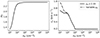 |
Fig. A.1. Variation in μp (left) and cs (right) with number density, nH, using one-dimensional models from 3D-PDR. The figure shows cs assuming both a constant μp and a variable μp. |
Figure A.2 shows the impact of a density-dependent cs and μp. Varying μp has a marginal impact: it enters weakly into the Jeans length and only deviates from a constant 2.33 in regimes where the gravitational component is anyway negligible. The impact of a variable sound speed is most noticeable at lower densities, increasing the gravitational component due to two reasons. First, as shown in Eq.10, increasing the sound speed will decrease the Mach number for a given σ0 and hence decrease nT. Second, the increased sound speed at low density increases the Jeans length (see Eq. 9). The result of both is that the Neff(H)−nH is brought slightly closer to the B23 fit. The most self-consistent method to include variable cs and μp is an iteration process between a photodissociation region model and the analytic relationship.
 |
Fig. A.2. Neff(H)−nH relationship modified by using a variable – cs(nH) (left), μp(nH) (middle), or both cs(nH) and μp(nH) (right). |
Appendix B: Power-law index of the Neff(H)−nH relationship
Previous works, such as Van Loo et al. (2013) and Safranek-Shrader et al. (2017), fitted the results from their three-dimensional simulations for a polynomial expression for Neff(H)−nH in dense gas. We calculated the slope of the analytic expressions from the derivative d log Neff/d log nH to examine the behavior in the asymptotic limits and transition regimes using the NUMPY gradient function.
Figure B.1 shows the computed slopes across the parameter space in Table 1. All models, with the exception of high values of n0, have their slopes asymptote to the isothermal Jeans-only limit of 0.5 at high density. The power-law indices at intermediate densities are highly dependent on the assumed parameters due to changes in where the transition between turbulence and gravitational regimes occurs. In models with lower σ0, the slope reaches a minimum between 103 ≤ nH ≤ 104, followed by a slight steepening of the slope toward 0.5. At low density, the model produces a range of super-linear power-law slopes from 1.5 to 2, with most of the solutions asymptoting around Neff ∝ n1.5, with n0 and αV being the most impactful. The average density, n0, is also the most impactful at the high density asymptotic limit.
The high-density power-law index asymptotes to  . This is close to the slopes computed from the simulation results discussed above, which found
  . This is explained in Fig. B.2, which compares the slope of the fiducial Neff(H)−nH to a linear fit in log-log space restricted to high density. While the constant fitted slope is consistent with previous works, the slope as a function of density varies between 0,3 and 0.6. The slightly flatter slope of the power-law fit is due to the inclusion of the turbulent column density component biasing the power-law slope fit to a flatter slope than a pure isothermal Jeans component.
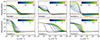 |
Fig. B.1. Same as Fig. 3 but showing the derivative, d log Neff/d log n. The horizontal lines show a slope of 0.4 and 0.5, which correspond to the results from hydrodynamic simulation fits (see text) and the isothermal Jeans-only limit. |
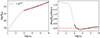 |
Fig. B.2. Comparison of the gradient calculation and a power-law fit in log-log space. Left: Neff(H)−nH relationship for the fiducial model (black), as shown in Fig. 2, and the polynomial fit for the dense gas (red). Right: Derivative, d log Neff/d log n, as a function of density (black). The power-law fit is shown with the horizontal line. The dense gas regime with nH > 103 is highlighted with a bold line. The power-law relationship is annotated at the top. |
All Tables
All Figures
|
Fig. 1. Chart showing the different components and where parameters enter into the model. |
| In the text | |
|
Fig. 2. Fiducial model results for the Neff(H)−nH relationship. The different components and totals are annotated. The red line shows the Bisbas et al. (2023) fit, and the band shows a factor of 2 deviation from it. The secondary y-axis shows the extinction using a scalar conversion factor as described in the text. “Total w/ biases” includes the resolution limit and floor. |
| In the text | |
|
Fig. 3. Parameter space results for the Neff(H)−nH relationship. In each panel the annotated parameter is varied but the others are fixed to the fiducial values given in Table 1. |
| In the text | |
|
Fig. A.1. Variation in μp (left) and cs (right) with number density, nH, using one-dimensional models from 3D-PDR. The figure shows cs assuming both a constant μp and a variable μp. |
| In the text | |
|
Fig. A.2. Neff(H)−nH relationship modified by using a variable – cs(nH) (left), μp(nH) (middle), or both cs(nH) and μp(nH) (right). |
| In the text | |
|
Fig. B.1. Same as Fig. 3 but showing the derivative, d log Neff/d log n. The horizontal lines show a slope of 0.4 and 0.5, which correspond to the results from hydrodynamic simulation fits (see text) and the isothermal Jeans-only limit. |
| In the text | |
|
Fig. B.2. Comparison of the gradient calculation and a power-law fit in log-log space. Left: Neff(H)−nH relationship for the fiducial model (black), as shown in Fig. 2, and the polynomial fit for the dense gas (red). Right: Derivative, d log Neff/d log n, as a function of density (black). The power-law fit is shown with the horizontal line. The dense gas regime with nH > 103 is highlighted with a bold line. The power-law relationship is annotated at the top. |
| In the text | |
Current usage metrics show cumulative count of Article Views (full-text article views including HTML views, PDF and ePub downloads, according to the available data) and Abstracts Views on Vision4Press platform.
Data correspond to usage on the plateform after 2015. The current usage metrics is available 48-96 hours after online publication and is updated daily on week days.
Initial download of the metrics may take a while.