Tight correlation of star formation with [CI] and CO lines across cosmic time

Theodoros Topkaras; Thomas G. Bisbas; Zhi-Yu Zhang; V. Ossenkopf-Okada

doi:10.1051/0004-6361/202451269

Home

All issues

Volume 701 (September 2025)

A&A, 701 (2025) A288

Full HTML

Open Access

Issue		A&A Volume 701, September 2025


Article Number		A288
Number of page(s)		18
Section		Extragalactic astronomy
DOI		https://doi.org/10.1051/0004-6361/202451269
Published online		24 September 2025

A&A, 701, A288 (2025)

Tight correlation of star formation with [CI] and CO lines across cosmic time

Theodoros Topkaras¹^⋆, Thomas G. Bisbas²^⋆, Zhi-Yu Zhang³^,4 and V. Ossenkopf-Okada¹

¹ I. Physikalisches Institut, Universität zu Köln, Zülpicher Str. 77, 50937 Köln, Germany
² Research Center for Astronomical Computing, Zhejiang Lab, Hangzhou 311100, China
³ School of Astronomy and Space Science, Nanjing University, Nanjing, China
⁴ Key Laboratory of Modern Astronomy and Astrophysics, Nanjing University, Ministry of Education, Nanjing, China

^⋆ Corresponding authors: topkaras@ph1.uni-koeln.de; tbisbas@zhejianglab.com

Received: 26 June 2024
Accepted: 13 August 2025

Abstract

Context. Cold molecular gas tracers, such as C I and CO lines, have been widely used to infer specific characteristics of the interstellar medium (ISM) and to derive star formation relations among galaxies.

Aims. However, there is still a lack of systematic studies of the star formation scaling relation of CO and [C I] lines across cosmic time on multiple physical scales.

Methods. We used observations of the ground state transitions of [C I], CO, and [C II], for 885 sources collected from the literature, to infer possible correlations between line luminosities of L′_[CI](1−0), L′_{CO(1 − 0)}, and L′_[CII] with star formation rates (SFRs). With linear regression, we fit the relations between SFR and molecular mass derived from CO, C I, and C II lines.

Results. The relation between [C I]- and CO-based total molecular masses is weakly superlinear. Nevertheless, they can be calibrated against each other. For α_CO = 0.8 and 4.0 M_⊙(K km s⁻¹ pc²)⁻¹ we derived α_[CI] = 3.9 and ∼ 17 M_⊙(K km s⁻¹ pc²)⁻¹, respectively. Using the lmfit package, we derived relation slopes of SFR–L′_{[CI](1 − 0)}, SFR–L′_{CO(1 − 0)}, and SFR–L′_{[CII](1 − 0)} to be β = 1.06 ± 0.02, 1.24 ± 0.02, and 0.74 ± 0.02, respectively. With a Bayesian inference linmix method, we find consistent results.

Conclusions. Our relations for [C I](1–0) and CO(1–0) indicate that they trace similar molecular gas contents, across different redshifts and different types of galaxies. This suggests that these correlations do not have strong evolution with cosmic time.

Key words: ISM: atoms / ISM: molecules / galaxies: evolution / galaxies: high-redshift / galaxies: ISM / galaxies: star formation

© The Authors 2025

Open Access article, published by EDP Sciences, under the terms of the Creative Commons Attribution License (https://creativecommons.org/licenses/by/4.0), which permits unrestricted use, distribution, and reproduction in any medium, provided the original work is properly cited.

This article is published in open access under the Subscribe to Open model. Subscribe to A&A to support open access publication.

1. Introduction

By studying the star formation rate (SFR) across different cosmic times and its correlation with other measurable quantities (Elbaz et al. 2011; Kennicutt & Evans 2012; Jo et al. 2021), the subsequent evolution and formation of galaxies can be unraveled (see McKee & Ostriker 2007, for a review). Some of the first quantitative SFR estimates were derived based on an evolutionary synthesis of galaxy colors (Tinsley 1968, 1972), followed by Kennicutt (1998a) who studied the SFR using measurements in far-infrared (FIR), ultraviolet (UV), and nebular recombination lines. The aforementioned works show that the cosmic SFR follows a hierarchy of physical processes. Objects spanning from megaparsec (Mpc) to kiloparsec (kpc) scales, for example the intergalactic medium (IGM) or spiral arms, collapse into smaller-scale structures leading to molecular cloud formation (Dobbs et al. 2014; Inutsuka et al. 2015). The IGM or spiral arms may collapse even further and fragment to form dense clumps on subparsec scales, and eventually progenitors of cores and planetary systems (Larson 1973; Boss 2001; Guszejnov & Hopkins 2016).

Previous studies estimated the SFR using extrapolated mid-infrared (mid-IR) or submillimeter observations (Calzetti et al. 2007; Kennicutt & Evans 2012; Simpson et al. 2015; da Cunha et al. 2015). More recent work, however, has shifted toward using the total infrared luminosity (L_IR, integrated over 8–1000 μm), which captures the emission from dust-obscured newly formed stars (Stacey et al. 2021; Montoya Arroyave et al. 2023). Although luminous infrared galaxies (LIRGs) were initially thought to be the dominant contributors to the cosmic SFR density at redshifts of z ∼ 1 (Chary & Elbaz 2001; Le Floc’h et al. 2005; Magnelli et al. 2009), later studies showed that more luminous sources, named ultra-luminous infrared galaxies (ULIRGs), with L_IR > 10¹² L_⊙, also contributed significantly at higher redshifts (z ≳ 2) (Daddi et al. 2007; Magnelli et al. 2009, 2011; Wang et al. 2019). Jo et al. (2021) examined the evolution of the cosmic SFR density across a wide redshift range (0 < z < 6), considering both major and minor contributors to star formation. Similarly, Elbaz et al. (2011), using FIR data from the Herschel Space Observatory (GOODS-Herschel key program), explored the SFR density and mid-IR continuum sizes. Both studies found that the SFR and L_IR follow a log-normal distribution with redshift, rising steeply at z < 2 and plateauing at z > 2. This reveals the tight correlation between SFR and L_IR (see Fig. 4 in Elbaz et al. 2011 and Fig. 2 in Jo et al. 2021).

The two most abundant cold molecular gas tracers are the ground state transition of ¹²CO(J = 1 − 0) at 115.27 GHz (hereafter CO(1–0)), and the ground state transition of [C I] (³P₁ − ³P₀) at 492.16 GHz (hereafter [C I](1–0)¹). Their correlation with SFR, namely the SFR–L′_{CO(1 − 0)} and the SFR–L′_{[CI](1 − 0)} relations, provide a comparison to the integrated Schmidt–Kennicutt (S-K) law (Schmidt 1959, see also Kennicutt & Evans 2012). The S-K law empirically links the surface density of cold gas to that of the star formation rate (SFR) expressed as Σ_SFR ∝ Σ_gas. This fundamental scaling relation (Schmidt 1959; Kennicutt 1998b) has been found to hold across a wide range of conditions, spanning several orders of magnitude both in Σ_SFR and Σ_gas. Notably, studies such as Gao & Solomon (2004a,b), Wu et al. (2005), Zhang et al. (2014a), Zhou et al. (2022) have reaffirmed that dense gas is more tightly related to star formation, compared to total neutral gas. For this work we examined the relationship between SFR and the luminosities of CO(1–0) and [C I][1–0]. Specifically, we tested the SFR–L′_{CO(1 − 0)} and SFR–L′_{[CI](1 − 0)} relations to evaluate the potential of these lines as reliable tracers of star formation.

CO molecular lines, particularly low-J transitions such as CO(1–0) and CO(2–1), are widely used to trace the cold H₂ content of the interstellar medium (ISM), providing a robust means of estimating the total molecular gas mass (Bothwell et al. 2013; Boogaard et al. 2020; Birkin et al. 2021; Montoya Arroyave et al. 2023). This is typically done by applying a CO-to-H₂ conversion factor, α_CO, to the observed CO(1–0) line luminosity (L′_{CO(1 − 0)}). A commonly adopted value for α_CO in the molecular ISM of disk galaxies (e.g., the Milky Way) is 4.3 M_⊙(K km s⁻¹ pc²)⁻¹ (Bolatto et al. 2013). In contrast, significantly lower values of α_CO ∼ 0.8–1.0 are typically used for more dynamically active systems, such as starbursts or galaxies hosting an active galactic nucleus (AGN), where elevated star formation rates and feedback processes may lead to higher excitation conditions (Downes & Solomon 1998). However, the universality of such a large difference in the value of the α_CO factor has been increasingly questioned (see recent works of Harrington et al. 2021; Dunne et al. 2022; Berta et al. 2023). This contrasts with earlier results from Downes & Solomon (1998), who based their conclusions on a small sample of low-J CO transitions in (U)LIRGs, potentially missing the warm, diffuse, and dense molecular gas present in local IR-luminous star-forming galaxies. This conversion factor has also been the subject of extensive investigation through observational studies Magdis et al. 2011; Jiao et al. 2021; Teng et al. 2022 and through numerical models (Feldmann et al. 2012; Gong et al. 2020; Bisbas et al. 2021), as it is known to depend strongly on environmental conditions in the ISM, such as far-UV (FUV) radiation field strength and cosmic ray ionization rate (see also review by Bolatto et al. 2013). In addition, it is known to be sensitive to metallicity (Genzel et al. 2012; Shi et al. 2016; Schruba et al. 2017), and appears to have smaller values at galactic centers (Bolatto et al. 2013). Sandstrom et al. (2013), for instance, showed that α_CO values in galactic centers can be up to a factor of ∼2 lower than galaxy-wide averages, though the weak correlation with metallicity in their sample suggests that other ISM properties (e.g., high gas temperatures) play a significant role.

The fine structure emission of atomic carbon, [C I](1–0), can also be used to infer the ISM characteristics (Papadopoulos et al. 2004; Walter et al. 2011; Valentino et al. 2018, 2020; Harrington et al. 2021). A significant difference compared to CO is that [C I](1–0) is mostly optically thin (Ikeda et al. 2002; Pérez-Beaupuits et al. 2015a; Harrington et al. 2021), while CO transitions are typically optically thick, with τ ≥ 10 at Σ_SFR > 1 Myr⁻¹ kpc⁻² (Narayanan & Krumholz 2014). In addition, the increasing contribution of the cosmic microwave background (CMB) radiation with redshift, affects the [C I] emission to a lesser degree (Zhang et al. 2016). Furthermore, Bisbas et al. (2015) suggested that elevated cosmic-ray (CR) ionization rates (ζ_CR) can lead to the destruction of CO molecules while the gas remains H₂-rich. High star-forming environments are expected to have elevated ζ_CR (Luo et al. 2023), suggesting that [C I](1–0) could potentially measure the molecular gas content more accurately as opposed to low-J CO transitions, in those environments. Consequently, regions with enhanced SFR activity may eventually become deficient in CO emission, while simultaneously being amplified in [C I] and possibly [C II] (Papadopoulos et al. 2018). It is important to mention that the distribution of [C I] is influenced by CRs, aligning it with the distribution of CO in the H₂ gas clouds (Bisbas et al. 2015, 2017a). This is in contrast to [C I] being confined to a narrow transition layer between the CO-rich inner H₂ cloud areas and the [C II]-rich outer regions (Draine 2010), and has been supported by several studies, making [C I] a robust tracer for the molecular content of sources (Papadopoulos & Greve 2004; Offner et al. 2014; Bisbas et al. 2021; Dunne et al. 2022).

Ionized carbon, [C II], can also serve as a molecular gas and SFR tracer (Olsen et al. 2017; Lagache et al. 2018; Khusanova et al. 2021; Ramos Padilla et al. 2021; Burgarella et al. 2022; Glazer et al. 2024). [C II] has the advantage of being one of the brightest lines to originate from star-forming regions (Brauher et al. 2008). It is a result of the interaction between the FUV photons and the interstellar medium (ISM) under typical ISM conditions. Velusamy & Langer (2014) and Accurso et al. (2017) showed that ∼60–85% of the total [C II] emission arises from the molecular gas phase, which closely links it with star-forming regions. As a SFR tracer, [C II] provides the advantage of being easily observed in a single frequency tuning, compared to total infrared measurements, which require multi-wavelength observations with different facilities. Despite the SFR – [C II] correlation, the “C II deficit” is present. This effect refers to the weaker-than-expected observed [C II] emission from FIR in sources with enhanced star formation activity. Since [C II], one of the brightest FIR lines, is associated with the presence of FUV radiation, it would be expected to be as bright as the FIR continuum. This C II deficit is a complex problem that has been intensively investigated for more than a decade (Graciá-Carpio et al. 2011; Sargsyan et al. 2012; Casey et al. 2014; Lagache et al. 2018; Bisbas et al. 2022; Lahén et al. 2022; Liang et al. 2023).

This study investigates the possible correlation between SFR and $L'_{[CI] ((1 - 0)}$ $\rm L{\prime}_{[CI]((1-0)}$ and $L'_{CO ((1 - 0)}$ $\rm L{\prime}_{CO((1-0)}$ , and the redshift dependence of these relationships. We used a large sample of sources (885 sources in total) with redshifts spanning 0 < z < 6.5. We also discuss the correlation of SFR with $M {(H_{2})}^{[C I]}$ $\mathrm M(H_2)^{[CI]}$ , $M {(H_{2})}^{CO}$ $\mathrm M(H_2)^{CO}$ , and lastly, we dedicate a small section to discussing the SFR– $L'_{[CII]}$ $\rm L{\prime}_{[CII]}$ correlation. Section 2 presents and describes our sample compilation, providing details of the sources. In Sect. 3 we present the results of our analysis. We further discuss the impact and reliability of the molecules used for the calculation of the SFR in Sect. 4. Finally, we summarize our conclusions in Sect. 5. For this work we adopted a ΛCDM cosmology, with H₀ = 67.8 km s⁻¹ Mpc⁻¹, Ω_M = 0.308, and Ω_Λ = 0.692 (Planck Collaboration XVI 2014), and a Salpeter initial mass function (IMF) (Salpeter 1955).

2. Sample selection

Our sample is a broad collection of sources from Walter et al. (2011), Alaghband-Zadeh et al. (2013), Sharon et al. (2016), Bothwell et al. (2017), Valentino et al. (2018, 2020), Harrington et al. (2021), Montoya Arroyave et al. (2023), Dunne et al. (2021, 2022), Berta et al. (2023), Castillo et al. (2025) (see Appendix B for details on the sample). We also include a small sample of sources with [C II] observations, reported in Cormier et al. (2015), Olsen et al. (2017), Glazer et al. (2024). The aforementioned works explore properties of the ISM, such as molecular mass, luminosity, brightness temperature ratios, including photodissociation region (PDR) properties, such as the UV-radiation field strengths, gas densities (n), gas temperatures, and possible scaling relations. Statistics considering the lines used and the number of sources taken from each work are presented in Appendix B. Finally, Fig. 1 displays the redshift distribution of our sample (only the CO and [C I] samples (see below)).

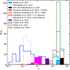Fig. 1.

Redshift distribution for our sample.

To maintain a level of homogeneity, all data were selected to have observations of both CO(1–0) and [C I](1–0) emission lines (except for the sources where we only used [C II] observations (i.e., Cormier et al. 2015; Olsen et al. 2017; Glazer et al. 2024 samples)). However, South Pole Telescope (SPT) dusty star-forming galaxies (DSFGs) (Bothwell et al. 2017) and the z-GAL survey galaxies (Berta et al. 2023), have only CO(2–1) data next to the [C I](1–0) observations. Also, the sample presented in Valentino et al. (2020) contains a small number of sources having only observations of CO(2–1) instead of CO(1–0. Thus, for a small number of galaxies used in this work (56 sources), the CO(2–1) transition was utilized. The CO(2–1) data were converted to CO(1–0) intensities (see Sect. 3.3 for more details). We chose to also include the CO(2–1) transition since both CO(1–0) and CO(2–1) are emitted under similar gas temperature (T_ex ∼ 5.5, 16.6 K for CO(1–0) and CO(2–1), respectively) and density (n_crit = 2.2 × 10³, 2.2 × 10⁴ cm⁻³ for CO(1–0) and CO(2–1), respectively). Higher-J CO transitions (e.g., CO(3–2)) reported in the literature are not taken into account here, as they generally trace warmer and denser gas.

Due to the nature of the sample, an overlapping listing effect is present across our literature samples (see details below). This overlapping listing effect has been taken into account in all calculations presented here. Literature data taken include redshifts, magnification factors (in the case of lensed sources), intensities (I_(CI](1−0), I_CO(1−0), I_CO(2−1), and I_[CIII]), and total-infrared luminosities. Using those data quantities such as $L'_{[CI] ((1 - 0)}$ $\rm L{\prime}_{[CI]((1-0)}$ , $L'_{CO ((1 - 0)}$ $\rm L{\prime}_{CO((1-0)}$ , $L'_{[CII]}$ $\rm L{\prime}_{[CII]}$ , $M {(H_{2})}^{[C I]}$ $\mathrm M(H_2)^{[CI]}$ , $M {(H_{2})}^{CO}$ $\mathrm M(H_2)^{CO}$ , and SFRs were computed.

Considering the large sample utilized, a certain level of inhomogeneity is expected (single-dish observations versus interferometric observations, flux extraction, lensed sources, weighted mean of some measurements). The numbers presented in this work and those mentioned in Walter et al. (2011), Alaghband-Zadeh et al. (2013), Sharon et al. (2016), Bothwell et al. (2017), Valentino et al. (2018, 2020), Harrington et al. (2021), Dunne et al. (2021), Dunne et al. (2022), Montoya Arroyave et al. (2023), Berta et al. (2023), Castillo et al. (2025), could potentially have minor differences due to the selected cosmology or IMF choice.

Last, we present a rather small sample of sources with [C II] observations (Cormier et al. 2015; Olsen et al. 2017; Glazer et al. 2024), along with the Bothwell et al. (2017) sample that also includes [C II] observational data.

Below, a summary of the selected galaxy sample compilation is presented. Despite the concise details provided below, we strongly suggest referring to each work as their authors provide information for values that are not addressed in this work (e.g., brightness temperature ratios, conversion factor investigation, PDR modeling).

From the combined sample of Walter et al. (2011), Alaghband-Zadeh et al. (2013), Sharon et al. (2016), eleven sources have been selected based on our criteria. Both CO(1–0) and [C I](1–0) measurements were used, by cross-matching the samples presented in Walter et al. (2011) and Sharon et al. (2016). Only one source (SMM J163650+4057) has an upper limit on the [C I](1–0) line. This sample is comprised of typical submillimeter galaxies (SMGs) with redshifts span of z ∼ 2.5–4. The observations were taken using the IRAM 30m, IRAM Plateau de Bure, and VLA. Some of the sources have previously been presented in Riechers et al. (2011a,b,c), Hodge et al. (2014), using CO(1–0) or [C I](1–0) observations separately. The majority of the sample (7/11) are gravitationally or strongly gravitationally lensed, with magnification factors of μ ∼ 2.5–80. We note that previously reported upper limits of GN20 (Daddi et al. 2009a; Casey et al. 2009) have been replaced with the new IRAM NOEMA detection presented in Cortzen et al. (2020). In this work, we will refer to this sample as Walter et al. (2011) for abbreviation, as they had the first publication reporting the majority of the sources.

Cormier et al. (2015) sample comprises 43 low-metallicity star-forming (SF) galaxies of the guaranteed time key program Dwarf Galaxy Survey (DGS) conducted with the PACS instrument on Herschel. Note that from the compact and extended samples presented in their work, only the compact sample was considered, as the latter sources were not fully mapped. The redshifts of this sample have a span of z = 0.00034 − 0.04539.

Bothwell et al. (2017) sample comprises 13 strongly gravitationally lensed sources found in the 1.4 mm blank-field survey with the South Pole Telescope, with redshifts ranging between z ∼ 3–4.7. These 13 sources were part of the Atacama Large Millimeter/submillimeter Array (ALMA) blind redshift search program (Weiß et al. 2013), including observations of ground-state, low- and high-J CO transitions. In that program, 26 SPT DSFGs were observed, as part of the Cycle 0 ‘early compact array’ setup, across the entirety of ALMA Band 3 (84–116 GHz). Bothwell et al. (2017) reported the [C I](1–0) transition, with only one source (SPT0345-47) as a nondetection. In addition, two more sources (SPT0300-46 and SPT2103-60) have a tentative detection of ∼3σ for the [C I](1–0) transition. Sources from this sample do not have observations of the CO(1–0) transition; instead, the reported CO(2–1) transition was utilized for the purposes of this work (see Sect. 3.3 for the method used to do the conversion). For this sample, we also used the reported [C II] data.

The sources taken from Olsen et al. (2017) were the 37 sources with z ≥ 5 that had [C II] observations. See Olsen et al. (2017) (and references therein) for further details in this sample, as the sources were previously reported in other works.

Valentino et al. (2018, 2020) sample comprises local-IR luminous galaxies, high-z main-sequence galaxies, SMGs and QSOs (see references therein for further details of the individual samples this sample comprises). Because the Valentino et al. (2018, 2020) sample includes sources from other samples utilized in our work (e.g., Walter et al. (2011) sample), an adjustment had to be made to exclude double-counted sources. Specifically, the local and high-z sources reported in Valentino et al. (2020) also include the Valentino et al. (2018) sample in its entirety. The high-z sources presented in Walter et al. (2011), Alaghband-Zadeh et al. (2013), Sharon et al. (2016), Bothwell et al. (2017) and four sources from the Harrington et al. (2021) sample are also included in the high redshift sample of Valentino et al. (2020). All the relevant sources from the aforementioned samples were excluded from the Valentino et al. (2020) sample used in the present work. This ensured that all sources used from Valentino et al. (2020) were unique for comparison. 11/76 high-z sources in Valentino et al. (2020) had CO(2–1) observations (see Sect. 3.3 for details of the conversion). Of the total of 217 sources, 76 have a [C I](1–0) detection and 30 have a CO(1–0) detection, leaving the remainder with either an upper limit or nondetection (see Appendix B for details). We also note that the sources taken from Valentino et al. (2020) were cross matched between data presented in Liu et al. (2015) and Kamenetzky et al. (2016a). For sources with several estimates of the same low J-CO transition, the line flux was represented by a S/N-weighted average.

Harrington et al. (2016, 2021) sample is part of the 24 strongly lensed Planck selected sources presented in Harrington et al. (2021). It was originally selected by the cross-match of Herschel and Planck 875 GHz detections (Harrington et al. 2016), and also 857, 545 and/or 353 GHz Planck detections. In addition, these galaxies were chosen based on their high far-infrared luminosities ( $L_{IR} = (0.22 - 14.6) \times 10^{12} L_{⊙}$ $\rm L_{IR} = (0.22{-}14.6) \times 10^{12}\,\, \rm L_{\odot}$ ), which indicate high SFRs. 17/24 sources were selected that have both [C I](1–0) and CO(1–0) observations, with a redshift range of z ∼ 1.1–3.5. Previous results (Harrington et al. 2016) suggest that despite the extreme L_IR, most of it is due to high star formation activity and not dust-obscured AGN activity. Therefore, their characteristics suggest that the sources span over a region above main-sequence sources for their redshift values, classifying them as starburst objects.

Dunne et al. (2021, 2022) have an extensive sample (312 sources in total) that includes high-z SMGs, local star-forming galaxies, (U)LIRGs, normal z = 1 and 0.04 < z < 0.35 galaxies. The sample contained lensed sources, sources with [C I] data taken with the Herschel Fourier Transform Spectrometer (FTS), and sources with only CO(2–1) observations. The Dunne et al. (2022) sample includes also the 12 250-μm selected galaxies at z = 0.35 reported in Dunne et al. (2021). Dunne et al. (2022) selected the sources from previous literature publications to have all three main molecular gas tracers, namely CO(1–0), [C I](1–0), and the submm dust continuum emission. Several sources included in Dunne et al. (2022) have also been reported in other samples used in this work. Namely, the sources presented in Walter et al. (2011), Bothwell et al. (2017), Valentino et al. (2018, 2020), Harrington et al. (2021) were excluded from the Dunne et al. (2022) sample presented in this work.

Montoya Arroyave et al. (2023) sample comprises 40 local (U)LIRGs, with a redshift range of z ∼ 0.007–0.19. The sources had both new and archival Atacama Pathfinder Experiment (APEX), and archival interferometric ALMA/Morita Array (ACA) observations. Montoya Arroyave et al. (2023) selected their sample based on previously reported (Veilleux et al. 2013; Spoon et al. 2013) Herschel OH 119 μm observations, investigating molecular outflows. 16/40 sources and 22/40 have [C I](1–0) and CO(1–0) observations, respectively.

The z-GAL sample (project IDs M18AB and D20AB; PIs: P. Cox, H. Dannerbauer, and T. Bakx) and the Pilot program (project IDs W17DM and S18CR; PI: A. Omont; Neri et al. 2020), which together observed 137 Herschel-selected sources with the IRAM Northern Extended Millimeter Array (NOEMA) and were presented in Berta et al. (2023), were also included in this work. The initial data release (Cox et al. 2023) reported the survey details and the initial results (e.g., spectroscopic redshifts, right ascensions, declinations). Ismail et al. (2023) continued by reporting the dust properties of the sample. Several of the targets have been resolved into multiple objects. This accounts for the identification of 178 individual galaxies with a redshift span of 0.8 < z < 6.5. Five sources are excluded from this sample (HerBS-204, HerS-18 W, HerS-19 SE, HerS-19 W, and HerS-9), since information regarding their spectroscopic redshift was missing. This brings the total sample used in this work to 173 sources. Cox et al. (2023) and Berta et al. (2023) reported the [C I](1–0) transition and additionally a selection of higher-J CO transitions from J_up = 2 to J_up = 8. Based on their reported data we only utilize the CO(2–1) transition (see Sect. 3.3 for the method used to do the conversion), ignoring all of the higher-J transitions.

Castillo et al. (2025) sample comprises CO(1–0) and [C I](1–0) Karl G. Jansky Very Large Array (JVLA) observations of 20 unlensed DSFGs at redshifts of z = 2 − 5 and dust masses of $M_{d} = 1 - 10$ $\rm M_d = 1{-}10$ × 10⁹ M_⊙. The sample is part of a total of 30 sources observed with JVLA (Castillo et al. 2023). In the UKIDSS Ultra Deep Survey (UDS), Cosmological Evolution Survey (COSMOS), Chandra Deep Field North (CDFN), and Extended Groth Strip (EGS) fields from the S2CLS (Serjeant et al. 2017) and S2COSMOS (Simpson et al. 2019) surveys, a sample of sources found within 4 deg² of SCUBA-2 850 μm imaging was used for the initial source selection. The brightest of those sources have additional ALMA and NOEMA observations (Stach et al. 2018; Hill et al. 2018; Simpson et al. 2020; Birkin et al. 2021; Chen et al. 2022; Liao et al. 2024).

Glazer et al. (2024) sample presents new z ∼ 7 [C II] observations with ALMA, for three confirmed lensed Lya emitting galaxies. Of the three sources, only one had a 4-σ detection of [C II], while the remaining two reported with 3-σ upper limits. Additionally, further observations of 6 < z < 7 sources were included (Watson et al. 2015; Schaerer et al. 2015; Knudsen et al. 2016; Matthee et al. 2017, 2019; Bradač et al. 2017; Carniani et al. 2018; Bowler et al. 2018; Smit et al. 2018; Hashimoto et al. 2019; Bakx et al. 2020; Harikane et al. 2020; Wong et al. 2022; Molyneux et al. 2022; Fujimoto et al. 2024; Ferrara et al. 2022; Schouws et al. 2023; Heintz et al. 2023).

3. Results and analysis

3.1. Magnification corrections

Strong gravitational lensing distorts the lensed source while increasing its apparent brightness by a magnification factor (μ), which depends both on the mass of the intervening lens and the source/lens arrangement. As a large number of sources reported in this work range from marginally gravitationally lensed to strongly gravitationally lensed by a foreground galaxy, the effects of gravitational lensing have to be quantified and accounted for. To account for the magnification effect, when needed, we divided all computed numbers by a magnification correction factor corresponding to each particular source. We must note that most of the magnification factors used in this work have been computed using 870-μm data. Thus, we assume that the lensing models applied to these sources also apply to the cold molecular gas traced by [C I] and CO.

Due to the geometric nature of gravitational lensing, every individual location within a lensed object is equally amplified across all wavelengths (see Bartelmann 2010 for a review). However, this does not imply a uniform amplification across all wavelengths for the entire galaxy, since the extent of the emission varies between different tracers. Accurately determining the magnification of dust sources presents a challenge. Submillimeter dust emission occurs on larger scales, compared to molecular gas, typically tens to hundreds of parsecs. Consequently, sources of this size tend to have lower overall magnifications, particularly when the magnifications derived from optical observations are high (e.g., when the optical source is near a caustic). When a source is large, only a small portion of its area will be sufficiently close to a caustic to experience significant amplification, while the rest will be farther away and thus magnified to a lesser degree. This variation in magnification across different parts of the source is referred to as ‘differential magnification’ or ‘chromatic lensing’, and can introduce significant bias in the derived properties of strongly lensed sources (Serjeant 2012). Additionally, the finite extent of the background galaxy leads to variations in the magnification applied to different regions within the galaxy. Consequently, the observed spectral energy distribution (SED) (Blain 1999), as well as the ratios of the spectral lines (Downes et al. 1995; Serjeant 2012), may be distorted by this differential magnification if there are spatial variations in the physical conditions within the source, as highlighted by Blandford & Narayan (1992).

The phenomenon of differential lensing, which refers to the fluctuation of the magnification factor across an extended source, can affect the properties of strongly lensed sources. One consequence of differential lensing is that it tends to bias the measurements of CO excitation toward more compact regions, resulting in higher excitation levels, as noted by Hezaveh et al. (2012). This effect of differential lensing can distort certain apparent characteristics of the source. For instance, if the impact of differential lensing is significant, a lensed region with a temperature higher than the average will appear hotter than its true temperature. However, low-J transitions such as CO(1–0) and [C I](1–0) are generally less influenced by the effects of differential lensing, as they are well mixed with the molecular part of the ISM (Ikeda et al. 2002; Papadopoulos et al. 2004). This indicates that the underlying molecular gas and [C I] or CO exhibit similar brightness profiles and therefore their ratios remain unaffected by the effects of differential lensing. Unfortunately, there is limited observational evidence that suggests the presence of this impact on these transitions (Deane et al. 2013).

It is worth mentioning that Valentino et al. (2020) report two separate values regarding the magnification factors for the high-z sample, to correct the continuum emission and its properties (μ_cont and μ_gas), but the mean difference (∼1%) is not significant. Here, the gas magnification factors were adopted, for the corresponding sample as suggested by Valentino et al. (2020), to study the properties of the ISM. The magnification factors for all the other objects were taken from the individual works that were first presented. We note that the sample reported in Berta et al. (2023) does not have published magnification factors (Bakx et al., in prep.). Since their sample possibly contains several gravitationally lensed sources, a magnification correction is needed to correct for the lensing effects. For this reason, all sources taken from Berta et al. (2023) are treated as upper limits (see Fig. 2, and Fig. 3). All quantities given below (L′_{CO(1 − 0)}, L′_{[CI](1 − 0)}, $L'_{[CII]}$ $\rm L{\prime}_{[CII]}$ , $M {(H_{2})}^{[C I]}$ $\mathrm M(H_2)^{[CI]}$ , $M {(H_{2})}^{CO}$ $\mathrm M(H_2)^{CO}$ , and SFRs) have been de-magnified for lensing effects, wherever needed².

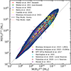Fig. 2.

$M {(H_{2})}^{[C I]}$ $\mathrm M(H_2)^{[CI]}$ vs. $M {(H_{2})}^{CO}$ $\mathrm M(H_2)^{CO}$ plot. The best fit using the lmfit package (red dashed line) and the linmix package (thick black solid line) are presented in the figure. The 1-to-1 line is presented as a dashed black line. Finally, the relation derived in Montoya Arroyave et al. (2023) ( $log M {(H_{2})}^{[CI]} = (1.21 \pm 2.42) + (0.91 \pm 0.25) log M {(H_{2})}^{CO}$ $\rm \log M(H_2)^{[CI]} = (1.21 \pm 2.42) + (0.91 \pm 0.25)\,\rm \log M(H_2)^{CO}$ ) is included as a dotted magenta line.

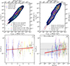Fig. 3.

L_IR vs. L′_{[CI](1 − 0)} (panel a), L′_{CO(1 − 0)} (panel b) luminosities, L′_{[CI](1 − 0)}/L′_{CO(1 − 0)} ratio against redshift (panel c), and L′_{[CI](1 − 0)}/L′_{CO(1 − 0)} ratio against L_IR (panel d). The secondary y-axis represents the SFR and the secondary x-axis the total molecular masses computed using the corresponding tracer. We include the best fit using the Levenberg–Marquardt algorithm of the lmfit package (red dashed line), and the Bayesian approach to linear regression using the linmix package (solid black line). In panel (b) we include the relations presented in Sargent et al. (2014) for main-sequence galaxies (thick black dashed line), and starburst galaxies (dash-dotted line). In panels (a) and (b), the relations derived in Montoya Arroyave et al. (2023) for CO(1–0) and [C I](1–0) line detections are presented (magenta dashed lines). Panels (c) and (d) include the lmfit and linmix method fits, with solid red and dashed black lines, respectively. In panel (d), the black dash-dotted line presents the mean L′_{[CI](1 − 0)}/L′_{CO(1 − 0)} value and the scatter (gray shaded area) derived by Gerin & Phillips (2000).

3.2. Regression models

In this work, a power law fit was performed using two regression models. The first model was implemented using the lmfit package of Astropy³. It utilizes a Levenberg-Marquardt algorithm (Gavin 2019) provided in the lmfit package, that solves the least squares problem accounting also for the errors of the sources in both axes and fits a user-supplied model to the supplied data. The second approach implements a Bayesian approach to linear regression using the linmix⁴ package (Kelly 2007), which also accounts for the errors in both axes. Bayesian reasoning is utilized, and a Markov chain is created with random samples from the posterior distribution. The progress of the Markov chain Monte Carlo (MCMC) method toward the posterior distribution is assessed using the potential scale reduction factor (RHAT), as introduced by Gelman (2004). Typically, a value of RHAT less than 1.1 indicates that an approximate convergence has been achieved. The propagation of the error, for both models, on the logarithmic axes have been taken into account as:

$\begin{matrix} Δ F = \frac{1}{ln 10} \frac{Δ x}{x}, \end{matrix}$ $\begin{aligned} \Delta \mathrm{F} = \frac{1}{\ln {10}} \frac{\Delta \mathrm{x}}{\mathrm{x}}, \end{aligned}$ (1)

where ln is the natural logarithm, Δ_x is the error of the corresponding value where x denotes the actual value, and Δ_F is the final computed error of the value.

3.3. Calculation of line luminosities

A small number of sources (see Sect. 2) lacked CO(1–0) observations. In those cases, the CO(2–1) transition was utilized for the calculations. A brightness temperature ratio was used to convert the intensity of the CO(2–1) line to the intensity of CO(1–0), with a value of r_21/10 = 0.84 ± 0.13 (Bothwell et al. 2013; Aravena et al. 2014). Although CO(2–1) represents a higher excited state of CO (with a three times higher critical density than CO(1–0), n_crit ≈ 7 × 10³ cm⁻³; Pérez-Beaupuits et al. 2015b), it remains an excellent tracer of the cold molecular gas, due to the low upper-level energy of 15 K. For this reason, it can be converted without introducing significant errors to the corresponding CO(1–0) intensities, assuming that the r_21/10 ratio remains approximately the same for different types of sources, and different environments. The latter assumption is in accordance to the recent numerical models of Bisbas et al. (2021) and within the errors of the value given in Bothwell et al. (2013) and Aravena et al. (2014). In particular, Bisbas et al. (2021) report a ratio of $r_{21 / 10, SF} / r_{21 / 10, nSF} = 1.5$ $r_{21/10,\rm SF}/r_{21/10,\rm nSF} = 1.5$ , for the two simulated clouds; a star-forming and a non-star-forming (see Wu et al. 2017).

Following the work of Solomon et al. (1997), Solomon & Vanden Bout (2005) we express the line luminosities in units of [K km s⁻¹ pc²] as:

$\begin{matrix} L_{line}' [{K km s}^{- 1} {pc}^{2}] = 3.25 \times 10^{7} ν_{rest}^{- 2} \frac{D_{L}^{2}}{1 + z} \int S_{v} d u . \end{matrix}$ $\begin{aligned} \mathrm{L}_{\rm line}\prime \,[\mathrm {K\,km\,s}^{-1}\,\mathrm{pc}^{2}] = 3.25 \times 10^{7} \,\nu _{\rm rest}^{-2} \frac{\mathrm{D}_{\rm L}^2}{1+\mathrm{z}} \int \mathrm{S}_{\rm v} du. \end{aligned}$ (2)

Here, ν_rest is the rest-frame frequency of the particular line in GHz, D_L is the luminosity distance of the source, in Mpc, and ∫S_vdu is the velocity (u) integrated flux of the observed line, in Jy km s⁻¹. Equation (2) represents the line luminosities proportional to brightness temperature (Solomon & Vanden Bout 2005).

3.4. Total molecular mass and SFR computations

Following the expression presented in Papadopoulos & Greve (2004), Dunne et al. (2022), the [C I](1–0) velocity integrated flux was used to calculate the total H₂ mass (without the contribution of He):

$\begin{matrix} M {(H_{2})}^{[CI]} [M_{⊙}] = \frac{0.0127}{χ_{C} Q_{10}} \frac{D_{L}^{2}}{1 + z} \int S_{[CI]} du \end{matrix}$ $\begin{aligned} \mathrm{M}(\mathrm{H}_2)^{[\mathrm{CI}]}\,[\mathrm{M}_{\odot }] = \frac{0.0127}{\chi _{\rm C} \mathrm{Q}_{10}} \frac{\mathrm{D}_{\rm L}^2}{1+\mathrm{z}} \int \mathrm{S}_{[\mathrm{CI}]} \mathrm{du} \end{aligned}$ (3)

where χ_C is the C/H₂ abundance ratio, and Q₁₀ (see Appendix A in Papadopoulos et al. 2004 for a detailed derivation of the equation excitation factor) is the fraction of carbon atoms in the first excited level, giving rise to [C I](1–0) emission. The factor ∫S_[CI]du represents the velocity integrated [C I](1–0) flux.

The equation implies that all carbon emission stems from molecular gas, an assumption that is justified by typical PDR models (Ossenkopf et al. 2007) and that allows us to compare the derived mass with the one obtained from CO. The excitation parameter Q₁₀ of atomic carbon has the advantage of being quite constant over a large range of temperatures and densities. A change in the excitation in denser or hotter gas mainly shifts the level population from the ground state to the upper state, leaving the intermediate one very stable. Papadopoulos et al. (2022) have shown that for typical ISM environments (n_H₂ = 300 − 10⁴ cm⁻³ and T_kin = 25 − 80 K) a value of Q₁₀ = 0.48 could be considered a typical value, as it varies little (∼16 per cent).

The abundance of atomic carbon relative to molecular hydrogen, χ_C, depends on many physical parameters of the galaxies (Papadopoulos et al. 2004). We followed a ‘standard’ literature approach utilizing the value presented in Weiß et al. (2003) and Papadopoulos & Greve (2004), adopting a C/H₂ abundance ratio of χ_C = 3 × 10⁻⁵ (or $α_{CI} = 6.6 M_{⊙} {(K km s^{- 1} {pc}^{2})}^{- 1}$ $\rm \alpha_{CI} = 6.6 \,{M_\odot}\, (K \,km\,s^{-1}\,pc^2)^{-1}$ ) for our derivations, but will discuss the parameter in more detail in Sect. 4.1. The use of a consistent value for the abundance ratio of the corresponding molecule is a crucial factor to calculate $M {(H_{2})}^{[C I]}$ $\mathrm M(H_2)^{[CI]}$ and subsequently to make comparisons between $M {(H_{2})}^{[C I]}$ $\mathrm M(H_2)^{[CI]}$ and $M {(H_{2})}^{CO}$ $\mathrm M(H_2)^{CO}$ .

The total H₂ mass using the CO(1–0) velocity integrated flux was calculated using:

$\begin{matrix} M {(H_{2})}^{CO} [M_{⊙}] = α_{CO} L_{CO (1 - 0)}', \end{matrix}$ $\begin{aligned} \mathrm{M}(\mathrm{H}_2)^\mathrm{CO}\,[\mathrm{M}_{\odot }] = \alpha _{\rm CO} \mathrm{L}_{\mathrm{CO}(1-0)}\prime , \end{aligned}$ (4)

and

$\begin{matrix} M {(H_{2})}^{[CI]} [M_{⊙}] = α_{CI} L_{[CI] (1 - 0)}', \end{matrix}$ $\begin{aligned} \mathrm{M}(\mathrm{H}_2)^{[\mathrm{CI}]}\,[\mathrm{M}_{\odot }] = \alpha _{\rm CI} \mathrm{L}_{[\mathrm{CI}](1-0)}\prime , \end{aligned}$ (5)

where α_CO and α_CI are the CO-to-H₂ and CI-to-H₂ conversion factors in units of M_⊙ (K km s⁻¹ pc²)⁻¹ (Solomon et al. 1997). Regarding the conversion factor, Bolatto et al. (2013) have shown that it depends on various physical effects such as temperature, metallicity, and cosmic rays. The latter two environmental parameters can severely underestimate the value of the conversion factor in the diffuse ISM as there is less dust shielding and lower levels of CO self-shielding, while the dense ISM remains CO-rich and bright. These effects lead to CO dissociation in the diffuse ISM, creating a significant amount of H₂ that is CO-dark (Bisbas et al. 2015, 2021, 2024; Papadopoulos et al. 2018, see also Sect. 4.2 for more discussion on this).

We start here with a CO-to-H₂ conversion factor of α_CO = 0.8 M_⊙ (K km s⁻¹ pc²)⁻¹ (Downes & Solomon 1998; Bothwell et al. 2017; Montoya Arroyave et al. 2023) as most of the studied sources are expected to have high (> 100 M_⊙ yr⁻¹) SFRs (see Sect. 4.1 for a discussion on that). This value is slightly lower than the α_CO ≃ 1 value commonly used for ULIRGs (Bolatto et al. 2013). This difference in the α_CO factor introduces a ∼25% increase difference on the individual $M {(H_{2})}^{CO}$ $\mathrm M(H_2)^{CO}$ . It is clear that α_CO has a large uncertainty from different studies. Recent studies even suggest a value of $α_{CO} = 4.0 M_{⊙} {(K km s^{- 1} {pc}^{2})}^{- 1}$ $\alpha_{\mathrm{CO}} = 4.0\,\mathrm{M}_{\odot}\,(\mathrm{K}\,\mathrm{km}\,\mathrm{s}^{-1}\,\mathrm{pc}^2)^{-1}$ , based on a large cross-calibrated sample of sources (Dunne et al. 2022). Since this work does not aim to investigate conversion factors (as in Dunne et al. 2022; Chiang et al. 2024; Ramambason et al. 2024), the specific choice of α_CO has little impact on our main premise.

Figure 2 shows a comparison of the calculated total molecular masses computed either from [C I] or CO using the two aforementioned conversion factors. We measure systematically larger $M {(H_{2})}^{[C I]}$ $\mathrm M(H_2)^{[CI]}$ compared to $M {(H_{2})}^{CO}$ $\mathrm M(H_2)^{CO}$ for the same source. This behavior has also been observed even in rather small samples (e.g., Walter et al. 2011; Bothwell et al. 2017) with similar types of sources (SMGs and QSOs) as the ones presented in this work. This could suggest i) a higher C/H₂ abundance ratio (assuming the same α_CO factor) or ii) a higher α_CO (assuming the same C/H₂) to explain the mass difference. Our fits approach the 1–1 line if we increase the C/H₂ to 5 × 10⁻⁵ (i.e., by a factor of 1.7), or vise versa if we increase the α_CO to 1.3 (i.e., by a factor of 0.6).

We also performed fits using the two methods presented in Sect. 3.2. All regression fits were performed using linear models in logarithmic space. Both fits are included in Fig. 1 with a red dashed line and a thick solid black line. The slope and intercept coefficients are presented in Table 1. They are almost identical within the errors. For comparison, the regression from Montoya Arroyave et al. (2023) is also included in Fig. 2, showing only a minor deviation from our results.

Table 1.

Slope and intercept values for the $M {(H_{2})}^{[C I]}$ $\mathrm M(H_2)^{[CI]}$ vs. $M {(H_{2})}^{CO}$ $\mathrm M(H_2)^{CO}$ relation.

Star formation rates are computed using the Kennicutt (1998a) SFR–L_IR relation, assuming a Salpeter initial mass function (IMF):

$\begin{matrix} SFR [M_{⊙} {yr}^{- 1}] = 1.71 \times 10^{- 10} L_{IR}, \end{matrix}$ $\begin{aligned} \mathrm{SFR} \,[\mathrm{M}_{\odot }\, \mathrm{yr}^{-1}] = 1.71 \times 10^{-10} \mathrm{L}_{\rm IR}, \end{aligned}$ (6)

where L_IR is the total-IR luminosity integrated over 8–1000 μm for the corresponding source. We note that the Harrington et al. (2021) sources had no calculations of L_IR but rather far-infrared luminosities, L_FIR, integrated from 40–120 μm spectra. To convert the L_FIR into L_IR a similar method as presented in Stacey et al. (2021) was followed. The reported L_FIR (Harrington et al. 2021) were multiplied by a factor of 1.91 (L_IR = 1.91 × L_FIR), following Dale et al. (2001), to account for the mid-infrared spectral features. Equation (6) was then used to calculate the SFRs. We note that Zhang et al. (2018) found evidence that starburst galaxies may contain a top-heavy IMF, different from the one assumed in this work. This may overestimate the values of SFR derived here, as a top-heavy IMF produces higher luminosities from the same mass of stars produced. This issue has also been addressed in Stacey et al. (2021) for their sources.

The values of L_IR used in this work are primarily taken from Valentino et al. (2020), except for the sources reported in Harrington et al. (2021), Dunne et al. (2021, 2022), Berta et al. (2023), Montoya Arroyave et al. (2023), and Castillo et al. (2025). In particular, Valentino et al. (2020) integrated (within 8–1000 μm) the SED using data available in the COSMOS spectroscopic coverage and a Draine & Li (2007) model. They also corrected the L_IR of SMGs for the AGN contribution (i.e., corrected for torus emission). Last, for QSOs, L_IR represents the SFR and the AGN contribution. This could overestimate the L_IR for the QSO sources included in Valentino et al. (2020) and subsequently our sample. We finally note that the L_IR values for Cloverleaf and RX J0911+0551 (Walter et al. 2011) were taken from Stacey et al. (2021) and have been converted to L_IR via the method presented above.

Ismail et al. (2023) measured the total infrared luminosity by integrating the modified black body (MBB) model for a range of 50–1000 μm. For this reason the Berta et al. (2023) sources’ L(50–1000 μm) were converted to L_IR(8–1000 μm) using a L(50–1000 μm) over L_IR(8–1000 μm) ratio of 0.7, derived using the SED template of Berta et al. (2013). We note here that the Berta et al. (2023) sources are likely lensed, so the L_IR(8–1000 μm) values could be overestimated due to lensing effects.

3.5. L′_[CI] and L′_CO correlation with total-IR luminosity and SFR

Our sample comprises an extensive, large, but still heterogeneous sample of galaxies. The large number of sources should minimize observational biases that typically favour high L_IR. While the independent observations can be biased (e.g., IR luminous sources, gravitationally lensed sources) our work tries to minimize this bias (on a statistical level) by using a large sample that contains sources with values of L_IR spanning ∼6 orders of magnitude (see Fig. 3). This means that potential underlying galaxy scaling relations capture our sample in its entirety, without biasing the derived linear regression slopes toward a specific range of sources. Montoya Arroyave et al. (2023) discuss this bias of small span in L_IR in their work, as their sample consisted only of local (U)LIRGs at similar redshifts (a similar discussion on the scaling relations is also addressed in Cicone et al. 2017). We note that although our sample has a significant L_IR span, for higher redshifts it can be biased to very bright sources. This is because both tracers (CO and [C I] lines) present observational challenges for sources with z > 4, due to high CR environments, turbulence, gas density, and metallicity (Bisbas et al. 2015, 2017b, 2021; Glover & Clark 2016; Papadopoulos et al. 2018; Clark et al. 2019).

SFR and L_IR calibrations are produced via two regression fits based on observable patterns:

$\begin{matrix} logSFR & = α_{sfr} + β logL'_{line}, \end{matrix}$ $\begin{aligned} \mathrm{logSFR}&= \alpha _{\rm sfr} + \beta \, \mathrm{logL}\prime _{\rm line},\end{aligned}$ (7)

$\begin{matrix} log L_{IR} & = α_{IR} + β logL'_{line}, \end{matrix}$ $\begin{aligned} \log \mathrm{L}_{\rm IR}&= \alpha _{\rm IR} + \beta \, \mathrm{logL}\prime _{\rm line}, \end{aligned}$ (8)

where SFR is the star formation rate of the source in units of M_⊙ yr⁻¹, L_IR is the total-IR luminosity of the source in units of L_⊙, and $L'_{line}$ $\rm L{\prime}_{line}$ is the prime line luminosity of each tracer ([C I](1–0), CO(1–0), or [C II]) in units of K km s⁻¹ pc². Finally, β and α are the slope and the intercept coefficients of the best fit, derived by one of the two used methods (see Sect. 3.2). Table 2 reports the derived values from the two models for [C I](1–0), and CO(1–0).

Table 2.

Slope, intercept, and dispersion values for the SFR (and L_IR in parentheses) vs. $L'_{[CI] ((1 - 0)}$ $\rm L{\prime}_{[CI]((1-0)}$ and $L'_{CO ((1 - 0)}$ $\rm L{\prime}_{CO((1-0)}$ relations.

Pearson correlation coefficients of 0.91 and 0.92 were derived for L_IR vs. L′_{[CI](1 − 0)} and L′_{CO(1 − 0)} relations, respectively. The Montoya Arroyave et al. (2023) relation ( $log L'_{[CI] (1 - 0)} = (- 6.42 \pm 4.91) + (1.27 \pm 0.40) log L_{IR}$ $\rm \log L{\prime}_{[CI](1-0)} = (-6.42 \pm 4.91) + (1.27 \pm 0.40)\, \log L_{IR}$ ) was also included in Panel (a) of Fig. 3, showing a shallower slope, compared to our values. Regarding Panel (b) of Fig. 3 the literature relations for main-sequence ( $log L'_{CO (1 - 0)} = (0.54 \pm 0.02) + (0.81 \pm 0.03) log L_{IR}$ $\rm \log L{\prime}_{CO(1-0)} = (0.54 \pm 0.02) + (0.81 \pm 0.03)\, \log L_{IR}$ ) and starburst galaxies ( $log L'_{CO (1 - 0)} = (0 . 08_{- 0.08}^{+ 0.15}) + (0.81) log L_{IR}$ $\rm \log L{\prime}_{CO(1-0)} = (0.08^{+0.15}_{-0.08}) + (0.81)\, \log L_{IR}$ ) presented in Sargent et al. (2014), and also the relation defined in Montoya Arroyave et al. (2023) ( $log L'_{CO (1 - 0)} = (0.8 \pm 0.22) + (0.74 \pm 0.18) log L_{IR}$ $\rm \log L{\prime}_{CO(1-0)} = (0.8 \pm 0.22) + (0.74 \pm 0.18)\, \log L_{IR}$ ) were included. Even though not all sources have enhanced star formation rates, even the starburst relation of Sargent et al. (2014) agrees with a difference in slope only of ∼0.5% with the lmfit model (∼5% with linmix).

Our derived relations for L_IR – L′_{CO(1 − 0)} lie between the two relations presented in Sargent et al. (2014) (MS and SB galaxies). As our sample contains both main-sequence and starburst sources, it can be self-explanatory as to why this is happening. The main-sequence and starburst relations of Sargent et al. (2014) and the relation derived in Montoya Arroyave et al. (2023) present a similar slope with the relations derived here. Without taking into account the sources of the Montoya Arroyave et al. (2023) sample, the main-sequence relation (Sargent et al. 2014) could be a good approximation for our sample compilation, despite the small difference in slope with our derived relations. On the contrary, the starburst relation is a better approximation for the Montoya Arroyave et al. (2023) sample, as their similarity can be considered negligible (the slope difference between Montoya Arroyave et al. (2023) relation and the SB relation from Sargent et al. (2014) is ∼9%). This is also self-explanatory as all the Montoya Arroyave et al. (2023) sample comprises local (U)LIRGs.

Panels (c) and (d) of Fig. 3 show the ratio of L′_{[CI](1 − 0)}/ $L'_{CO (1 - 0)}$ $\rm L{\prime}_{\mathrm{CO(1-0)}}$ against redshift and L_IR, respectively. Both panels display a broad range along the y-axis, with no clear indication of a distinct trend (panel (c): b = 0.029 ± 0.011, and 0.046 ± 0.017, for lmfit and linmix, respectively, panel (d): b = 0.057 ± 0.015, and 0.075 ± 0.017, for lmfit and linmix, respectively). We derive a mean ratio of L′_{[CI](1 − 0)}/ $L'_{CO (1 - 0)} = 0.22$ $\rm L{\prime}_{\mathrm{CO(1-0)}} = 0.22$ ± 0.07, and Pearson correlation coefficients of 0.24 and 0.27 for panel (c) and (d), respectively. We also present the mean value (L′_{[CI](1 − 0)}/ $L'_{CO (1 - 0)} = 0.2$ $\rm L{\prime}_{\mathrm{CO(1-0)}} = 0.2$ ± 0.2) for a sample of local spirals, mergers, and low-metallicity galaxies, as described in Gerin & Phillips (2000). Despite the large dispersion, our mean value is close to that of Gerin & Phillips (2000). [C I](1–0) and CO(1–0) are strongly correlated independent of galaxy type and redshift, and a very weak dependence on L_IR only, given the large scatter. Finally, although we expected some metallicity dependence, we found none, assuming that metallicity also evolves with redshift.

Figure 3 (panels (a) and (b)) shows that both L′_{[CI](1 − 0)} and $L'_{CO (1 - 0)}$ $\rm L{\prime}_{ CO(1-0)}$ are tightly correlated with L_IR and SFR. We note that sources that had upper limits for SFR, L_IR, L′_{[CI](1 − 0)} and L′_{CO(1 − 0)} were also taken into account for the fitting. To account for these sources a conservative error of 20% of the reported value was assumed (this will be further discussed in Sect. 4.2). This enabled us to include upper limits to the fitting algorithms, thus utilizing the majority of sources from our sample.

3.6. SFR vs. L′_[CII] relation

As mentioned in Sect. 1, [C II] also traces the SFR as it measures the UV irradiation from young massive stars independent of the amount of molecular material. Although most of the sources used here lacked [C II] observations, the SPT sources (Bothwell et al. 2017) offered a small sample to further extend previous fitting relations to larger values of SFR and $L'_{[CII]}$ $\rm L{\prime}_{[CII]}$ . Additionally, literature observational data presented in Cormier et al. (2015) and Olsen et al. (2017), as well as recent ALMA observations (Glazer et al. 2024) were included. We note that Olsen et al. (2017) calculated their SFR using a Chabrier IMF, so their reported numbers have been multiplied by a factor of 1.6, to account for the Salpeter IMF used here. A best-fit relation was derived by using the two aforementioned regression models (see Sect. 3.2), and presented in Fig. 4 as a solid red and a black dashed line.

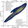Fig. 4.

SFR vs. $L'_{[CII]}$ $\rm L{\prime}_{[CII]}$ for the samples of Cormier et al. (2015) (green triangles), Olsen et al. (2017) (orange triangles), Bothwell et al. (2017) (black squares), and Glazer et al. (2024) and references therein (red symbols and teal stars). The red solid line represents the best fit for the listed sample based on a Levenberg–Marquardt algorithm, and the thick black dashed line represents the Bayesian fitting. The gray, black, and blue dashed lines represent different best-fitting relations presented by Herrera-Camus et al. (2015), Pineda et al. (2014), and Sutter et al. (2019), respectively. In addition, we plot with solid black, blue, and green lines the De Looze et al. (2014) Dwarf Galaxy Survey (DGS), and the normal and high star formation efficiency relations by Herrera-Camus et al. (2018) (HC+ 2018), respectively. The relation given in Bisbas et al. (2022) is presented as a dashed magenta line. Finally, the relation that best fits the simulated data presented by Olsen et al. (2017) is included in the figure with a dash-dotted yellow line.

Figure 4 further includes literature best-fitting relations (De Looze et al. 2014; Pineda et al. 2014; Herrera-Camus et al. 2015, 2018; Olsen et al. 2017; Sutter et al. 2019; Bisbas et al. 2022). Herrera-Camus et al. (2015) reported in the Herschel KINGFISH sample of 46 nearby galaxies, investigating the correlation of [C II] surface brightness and luminosity with the SFR of the corresponding sources. They followed an ordinary least squares (OLS) linear bisector method to best fit their data. This relation is presented with a dashed gray line. Pineda et al. (2014) investigated the relation between [C II] and SFR in the Galactic plane, by comparing their results with the Large Magellanic Cloud (LMC), galaxies studies in De Looze et al. (2011), and for individual PDRs. This relation is depicted with a black dashed line. The blue dashed line corresponds to the relation derived by Sutter et al. (2019), who presented a sample of Herschel KINGFISH and Beyond the Peak programs data for 31 nearby sources that had both [C II] and [N II] 205 μm spectral maps. The relation investigating the applicability of [C II] fine-structure line as a SFR tracer presented in De Looze et al. (2014) is included in the best-fitting relations with a solid black line. Both normal and high star formation efficiency (SFE) relations presented in Herrera-Camus et al. (2018) using Herschel/PACS observations of the main far-infrared (FIR) fine-structure lines are also included, with solid blue and green lines, respectively. The relation that best fits the simulated galactic data (Olsen et al. 2017) produced with SÍGAME (SImulator of GAlaxy Millimeter/submillimeter Emission) is included with the dashed yellow line. This relation is derived by fitting the simulated multiphased ISM for 30 main-sequence galaxies at a redshift of z ∼ 6, with a rather small SFR (∼3–23 M_⊙ yr⁻¹). Those 30 simulated galaxies are not included in Fig. 4. Finally, the relation fitting the synthetic [C II] observations of smoothed particle hydrodynamics (SPH) simulations of a dwarf galaxy merger presented in Bisbas et al. (2022) is given with a dashed magenta line. We note that the aforementioned literature fittings were performed for SFR vs. L_[CII] in solar luminosity units (L_⊙). For this reason, a complementary x-axis denoting L_[CII] was added in Fig. 4.

The best-fitting relations from our models that correlate the sources presented in Fig. 4 are presented with a solid red and a thick black dashed line. A similar method was followed to the one previously used for SFR – L′_{[CI](1 − 0)} and SFR – L′_{CO(1 − 0)} (see Fig. 3), using the lmfit and linmix packages. The derived slope and intercept coefficients are presented in Table 3.

Table 3.

Slope, intercept and dispersion values for the SFR vs. $L'_{[CII]}$ $\rm L{\prime}_{[CII]}$ relation.

From the literature best-fit relations presented in Fig. 4, the one derived by De Looze et al. (2014) and the high SFE relation by Herrera-Camus et al. (2018) have similar slopes with both our data and our derived relations (red solid and black dashed line). The De Looze et al. (2014) relation has a ∼13% difference in slope with the lmfit relation and a ∼15% difference in slope with the linmix relation. The slope of the high SFE relation by Herrera-Camus et al. (2018) differs from the lmfit and linmix relations by ∼35% and ∼36%, respectively. The normal SFE relation of Herrera-Camus et al. (2018) also presents merit, following a similar slope toward high $L'_{[CII]}$ $\rm L{\prime}_{[CII]}$ . This relation deviates to smaller SFRs toward the lower left part of Fig. 4. Although a number of the aforementioned relations (Herrera-Camus et al. 2015; Sutter et al. 2019) appear to give good results (less than ∼30% difference with our models) toward the high SFR and high $L'_{[CII]}$ $\rm L{\prime}_{[CII]}$ end of Fig. 4, they present higher deviation at the low SFR and low $L'_{[CII]}$ $\rm L{\prime}_{[CII]}$ end. The Pineda et al. (2014) relation has the largest deviation for both high and low SFR, suggesting that it is not a good approximation for the sample used here (although it follows a prominent slope for the low SFR and low $L'_{[CII]}$ $\rm L{\prime}_{[CII]}$ end of Fig. 4, it fails to approximate the higher-end part).

The new observations presented in Glazer et al. (2024) are also included in Fig. 4. Of these three sources, only one (MACS0454-1251) had a 4σ detection of [C II], while the remaining two sources (RXJ1347-018 and MACS2129-1412) exhibit only upper limits. Glazer et al. (2024) also discuss how low metallicity could shift galaxies below certain SFR– $L'_{[CII]}$ $\rm L{\prime}_{[CII]}$ relations, as observed for the two upper limit galaxies presented in the corresponding work (and for a large majority of the upper limits utilized). This effect can also be observed for a large majority of z > 6 sources that are included in Fig. 4 (teal stars, corresponding to galaxies with 6 < z < 7). Curti et al. (2024) addressed this effect and suggested that lower mass sources at redshifts z > 6 exhibit subsolar metallicities, effectively destroying star-forming sites (Vallini et al. 2015; Ferrara et al. 2019). Our models also agree with the finding of Glazer et al. (2024) regarding MACS2129-1412, concluding that this source is within 1σ scatter from the De Looze et al. (2014) SFR– $L'_{[CII]}$ $\rm L{\prime}_{[CII]}$ relation. Considering our modeling, both MACS0454-1251 and the upper limit for RXJ1347-018 ( $L_{[CII]} = 0.043 \times 10^{8} L_{⊙}$ $\rm L_{[CII]} = 0.043 \times 10^{8}\,L_{\odot}$ ) are within ∼3σ scatter from our two linear regression models. Following the one diverging source (MACS2129-1412), a large majority of the 6 < z < 7 sources (teal stars) lie well below or above our models and additionally from the De Looze et al. (2014) relation, suggesting that the [C II] deficit could play a more significant role for these sources (Vallini et al. 2015; Bisbas et al. 2022). However, the majority of the sources are upper limits on either SFR and/or $L'_{[CII]}$ $\rm L{\prime}_{[CII]}$ . Even though our derived relations agree with previously reported values, their use of mostly upper limits as an input makes them unreliable for this sample.

4. Discussion

4.1. Total molecular masses and abundance ratios

A value for the C/H₂ (χ_C) abundance ratio of χ_C = 3 × 10⁻⁵ (Papadopoulos & Greve 2004; Bothwell et al. 2017; Montoya Arroyave et al. 2023) was used to compute the total molecular gas mass via the [C I] line. This value of the abundance ratio is the average of the minimums recorded in the Orion A and B clouds (∼10⁻⁵, Ikeda et al. 2002) and in the starburst environment of M82 nucleus (5 × 10⁻⁵, White et al. 1994). The recent study of Jiao et al. (2021) examined a sample of six nearby galaxies and suggested that the commonly adopted value for χ_C is well within the statistical variance of the sources examined in their corresponding work. Although Jiao et al. (2021) (and references therein) investigated only a small number of nearby sources, their derived value (C/H₂ = 2.3 × 10⁻⁵) agrees well with the value commonly adopted in the literature (i.e., 3 × 10⁻⁵). It will be useful, however, to explore how different values of this ratio affect the results.

A commonly used technique to benchmark two different tracers in estimating the total molecular gas mass is to keep one of the two fixed while changes are performed in the other one. Following this, by keeping α_CO fixed at 0.8 M_⊙(K km s⁻¹ pc²)⁻¹ we vary the C/H₂ ratio (or α_CI, see Eq. (5)) and re-calculate the H₂ gas masses traced by [C I]. As a large number of sources in our sample have relatively enhanced $L_{CO (1 - 0)}'$ $\rm L_{CO(1-0)}{\prime}$ , our choice of α_CO = 0.8 is a fair assumption. The opposite approach using a different α_CO will be discussed below. We find a good match of the masses if we increase the C/H₂ ratio by a factor of 1.6, so that C/H₂ = 5 × 10⁻⁵. This approach was also considered in Bothwell et al. (2017) finding a better agreement between the CO- and [C I]-traced H₂ gas masses by using an elevated C/H₂ ∼ 7 × 10⁻⁵. Castillo et al. (2025) followed a similar approach, deriving an abundance ratio of χ_C = 5.6 ± 2.0 × 10⁻⁵ and χ_C = 5.1 ± 1.8 × 10⁻⁵ when they separate their sample into two different redshift bins (z < 3.5, and z > 3.5). Evidently, an elevated C/H₂ ratio of 5 × 10⁻⁵ may be preferred for these types of galaxies, especially those with enhanced SFRs.

There are several reasons to expect elevated abundances of C in the ISM of these galaxies. High SFR environments would suggest high CR and a more turbulent environment (Papadopoulos 2010). CRs can penetrate deep into a cloud (Strong et al. 2007; Padovani et al. 2009; Grenier et al. 2015), making it C-rich via reactions caused by the presence of high abundances of He⁺ and H₃⁺, ions that are produced from the CR interaction (Bialy & Sternberg 2015; Bisbas et al. 2015, 2017b; Gaches et al. 2022). In addition, the astrochemical models of Bisbas et al. (2023) showed that the molecular mass content in column-density distributions similar to a star-forming ISM, is C-rich across a large span of CR ionization rates and metallicities, and even C-dominant in environments of a low FUV intensity. It is noted here, however, that the more recent PDR and radiative transfer models representing an α-enhanced low-metallicity star-forming cloud of Bisbas et al. (2024), show that low C/O ratios can severely suppress the [C I] emission while boosting the low-J CO one, leaving the H₂ abundance in the cloud unaffected. This suggests that a potential α-enhanced environment may have a significant effect in some of the targets presented here. It can affect the [C I] emission and subsequently the [C I] computed total molecular mass, without affecting the total SFR of the corresponding sources (see Michiyama et al. 2020, as an example of a [C I]-dark galaxy).

Instead of modifying the atomic carbon abundance, there are also arguments for a higher α_CO value than used here. Using a large heterogeneous sample (407 sources) of dusty star-forming galaxies, Dunne et al. (2022) found an α_CO = 4.0 ± 0.1 M_⊙(K km s⁻¹ pc²)⁻¹ (including helium) and a C/H₂ abundance ratio of 1.6 × 10⁻⁵. Since their sample is selected to have sources with FIR/sub-mm/mm wavelength it can be safely assumed that they have high- or comparable metallicities with the Milky Way, highlighting that metallicity can severely affect both the α_CO conversion factor and the C/H₂ abundance ratio values (Jiao et al. 2021; Bisbas et al. 2023, 2024, 2025). While these authors support those near-universal values for both α_CO and χ_C factors, many high-resolution studies of gas kinematics in SMGs cannot easily support this high value for α_CO based on their derived stellar and dynamical masses (Magdis et al. 2011; Riechers et al. 2020a; Birkin et al. 2021; Castillo et al. 2022; Amvrosiadis et al. 2025). Using χ_C = 5 × 10⁻⁵ (or α_CI = 3.94 M_⊙ (K km s⁻¹ pc²)⁻¹), and assuming α_CO = 0.8, yields consistent H₂ masses derived from both CO and [C I] across the sample. The resulting values imply that the majority of sources in our sample have solar or super-solar metallicities, as noted by Heintz & Watson (2020).

The α_CO conversion factor has been found to increase at low metallicity (Leroy et al. 2011; Genzel et al. 2012; Amorín et al. 2016; Shi et al. 2016) depending also on the density distribution (Schruba et al. 2017; Bisbas et al. 2021). In line with these findings are the recent works of Chiang et al. (2024) and Ramambason et al. (2024). In particular, Chiang et al. (2024) found α_CO = 4.2 M_⊙ (K km s⁻¹ pc²)⁻¹ using dust emission as a tracer of the gas surface density. Ramambason et al. (2024) performed representative modeling of the ISM using the Bayesian code MULTIGRIS in combination with low-metallicity dwarf galaxies observations and found that CO may not be a reliable H₂ gas tracer in low metallicity environments. The [C II] fine-structure line can be used as an alternative tracer in such cases (Zanella et al. 2018), and including the ISM environments of high CR ionization rates, as the α_CII conversion factor has been found to not strongly dependent on metallicity (Cormier et al. 2015; Madden et al. 2020; Bisbas et al. 2021; Hunter et al. 2024). In this regard, observations in the [C II] emission line are recently of popular interest, since it can be detected by ALMA in the high-z Universe.

Adopting an α_CO = 4.0 M_⊙ (K km s⁻¹ pc²)⁻¹, as suggested by Dunne et al. (2022), we find that the resulting total molecular masses require a C/H₂ abundance ratio of 1.2 × 10⁻⁵ to remain consistent. We calculate an α_CI ∼ 17 M_⊙(K km s⁻¹ pc²)⁻¹, a value similar to the one derived in Dunne et al. (2022). Despite this change in α_CO and C/H₂ abundance ratio, the resulting [C I]-based and CO-based total molecular masses fit derived in Fig. 2 still exhibits a super-linear behavior with a slope of ∼1.10, consistent with our previous analysis.

4.2. Comparison of L′_{CO(1 − 0)}-L_IR and L′_{[CI](1 − 0)}-L_IR with the literature.

Taking into account the assumptions and corrections that have been implemented to compute the total SFR and also the L′_{CO(1 − 0)} and L′_{[CI](1 − 0)} of the sources, we derived a close-to-linear correlation with SFR (see Sect. 3.5). We remind the reader that the SFR was computed for the majority of the sample using 8–1000 μm integrated total-infrared luminosity observations that were acquired using detailed SED integration (Valentino et al. 2020; Dunne et al. 2022; Berta et al. 2023). The sources presented in Harrington et al. (2021) had 40–120 μm integrated FIR observations, and therefore an extrapolation similar to the one presented in Stacey et al. (2021) was used to convert from L_FIR to L_IR (see Sect. 3.4). We also stress that possible IMF normalizations were taken into account for our computations. We provide a reminder of these assumptions as they are crucial in making meaningful and consistent comparisons of a large dataset such as the one used in this work.

Using a sample of 885 sources, we have shown that both [C I](1–0) and CO(1–0) luminosities correlate with the total SFR, over approximately 6 and 5 orders of magnitude, respectively (see Table 2). With a span in redshift covering 0 < z < 6.5, empirical relations with a slope of b = 1.06 ± 0.02 using the lmfit model (b = 1.16 ± 0.03 using the linmix model) was derived for the SFR– $L'_{[CI] (1 - 0)}$ $\rm L{\prime}_{\mathrm{[CI](1-0)}}$ relation. Similar coefficients were derived for the SFR–L′_{CO(1 − 0)} transition. A slope of b = 1.24 ± 0.02 was derived using the lmfit model (b = 1.17 ± 0.02 using the linmix model). As the final relations partially depend on upper limits that were taken into account for the fitting, a 20% error based on the corresponding original value was assumed; 10% following the Galametz et al. (2013) calibrations and an additional conservative 10% due to e.g., flux calibration errors, supernovae remnants that could potentially contribute to L_IR, and mergers (Hopkins et al. 2010). Although similar correlations have been discussed in previous works (Valentino et al. 2018, 2020; Montoya Arroyave et al. 2023), they were biased mostly toward the number and type of the adopted sources. Considering the potential bias of those previous work, their derived relations give similar trends, albeit with different slope values.

Based on a sample of 36 galaxies, Montoya Arroyave et al. (2023) provide a correlation between SFR and L′_{[CI](1 − 0)} or L′_{CO(1 − 0)} when no LIRGs contribution is taken into account, for a SFR range of ∼ 17 − 1183 M_⊙ yr⁻¹. We note that those correlations correspond to SFRs computed using a different method from the one utilized here. In particular, the authors calculated/taken literature values of SFR that use the expression presented in Sturm et al. (2011) and in Spoon et al. (2013) (namely $SFR = (1 - α_{AGN}) \times 10^{- 10} L_{IR}$ $\mathrm{SFR} = (1- \rm \alpha _{AGN}) \times 10^{-10} \rm L_{IR}$ , where α_AGN is the AGN contribution factor) accounting also for the AGN contribution. By using the richer sample of galaxies presented here, we find that this correlation (with slightly different slope values) can be used for a wider range of SFRs. This, in turn, implies that a meaningful correlation between SFR and L′_{[CI](1 − 0)} or L′_{CO(1 − 0)} can be derived with a wide span of values in redshift and L_IR.

Although the SFR–L′_{CO(1 − 0)} relation has been extensively studied in the literature (Gao & Solomon 2004a; Bayet et al. 2009; Juneau et al. 2009; Greve et al. 2014), there is a lack of similar works examining the SFR vs. L′_{[CI](1 − 0)} correlation. In addition, although extensive samples have been reported using CO(1–0) or [C I](1–0) observations to investigate the molecular content and/or the SFR (Leroy et al. 2005; Lisenfeld et al. 2011; Cicone et al. 2017; Valentino et al. 2018, 2020; Harrington et al. 2021; Dunne et al. 2021, 2022; Berta et al. 2023; Castillo et al. 2023), to our knowledge no comprehensive study combining both these tracers to such a wide redshift span has been previously made. Our study compares total molecular mass content and the SFR using both tracers from the same sources, thus minimize possible redshift biases. However, we have to address that the majority of the sources were selected using IR- and FIR-bright Herschel data, resulting in a large number of (U)LIRGs, starbursts, or low-metallicity dwarf galaxies. This can introduce a bias toward only the IR- and FIR-bright sources across our redshift range, especially for redshifts z > 4, as also explained in Sect. 3.5.

Bothwell et al. (2017), Valentino et al. (2020) and Montoya Arroyave et al. (2023) suggested that [C I] can give reliable results of the total molecular mass content of galaxies, and can be thus used as an alternative molecular gas tracer for local and extragalactic sources (Papadopoulos et al. 2004; Lo et al. 2014; Zhang et al. 2014b). Only recently and for a limited number of sources, Bothwell et al. (2017) and Montoya Arroyave et al. (2023) compared $M {(H_{2})}^{[C I]}$ $\mathrm M(H_2)^{[CI]}$ and $M {(H_{2})}^{CO}$ $\mathrm M(H_2)^{CO}$ and found a larger molecular content when using [C I](1–0). Figure 2 illustrates the larger sample selection used in this work and, as can be seen, agrees with their results. This supports the hypothesis that [C I](1–0) could trace larger quantities of cold molecular gas in local and high-z galaxies, compared to CO(1–0).

The discrepancy in $M {(H_{2})}^{[C I]}$ $\mathrm M(H_2)^{[CI]}$ and $M {(H_{2})}^{CO}$ $\mathrm M(H_2)^{CO}$ can also be explained by the ‘CO-dark’ gas (van Dishoeck 1990, 1992). The term ‘CO-dark’ refers to molecular regions that due to the lower self-shielding ability of CO compared to H₂, can remain H₂-rich but be CO-poor (Lada & Blitz 1988). This ‘CO-dark’ gas can be manifested as either due to the lack of CO molecules, existing in translucent or diffuse clouds in molecular regions due to the weaker CO emission (Seifried et al. 2020), or due to the low sensitivity limit of telescopes to detect the CO(1–0) rotational transition (Langer et al. 2014). A weaker CO emission can be compensated by raising the value of the α_CO conversion factor. However, since there is no information on the column density of CO, N(CO), we are unable to correct for the ‘CO-dark’ discrepancy using the α_CO.

Furthermore, the cosmic microwave background radiation (CMB) can have a severe impact on the computed total molecular mass using the CO(1–0) transition (Da Cunha et al. 2013; Zhang et al. 2016) for z > 4. This stems from the fact that the CMB increases in temperature, and therefore it becomes brighter at higher-z. Low-J CO lines, because of their low frequency, would be decreased after its radiation transfer with the CMB, showing much less contrast than their intrinsic line emission. This is especially severe for molecular gas with kinetic temperature below 20 K, while for warm gas with T_kin ∼ 50 K, this effect would decrease the CO line luminosity within 50% (Zhang et al. 2016). [C I] lines are much less affected by this CMB effect and therefore would be more robust for the high redshift Universe. The CMB effect increases both α_CO and α_CI, subsequently decreasing the corresponding tracer emission. This reduction in emission was explored in Castillo et al. (2025), which proposed a non-negligible decrease in both [C I](1–0) and CO(1–0) emission. However, this decrease appears to have a counteracting effect on the measured luminosity ratio, as reported by Castillo et al. (2025). Literature values considering high-z SMGs and ULIRGs, report log (L′_{[CI](1 − 0)}/ $L'_{CO (1 - 0)}$ $\rm L{\prime}_{\mathrm{CO(1-0)}}$ ) =−0.71 ± 0.12, while Valentino et al. (2018) report a value of log (L′_{[CI](1 − 0)}/ $L'_{CO (1 - 0)}$ $\rm L{\prime}_{\mathrm{CO(1-0)}}$ ) =−0.69 ± 0.16. Both literature ratios and our calculated one (see Sect. 3.5) are in close agreement. Furthermore, Jarugula et al. (2021) and Harrington et al. (2021) have measured high kinetic temperatures (T_dust ∼ 45 K, T_kin/T_dust ≈ 2.5) for a selection of strongly lensed sources with z > 4. This could explain the relatively minor effect of CMB in our high-z sample (slopes < 0.1, see Sect. 3.5, and Fig. 3).

4.3. [CII] as a SFR tracer

Numerous studies explore the ability of [C II] in tracing the SFR of galaxies (De Looze et al. 2014; Pineda et al. 2014; Cormier et al. 2015; Olsen et al. 2017; Herrera-Camus et al. 2018; Sutter et al. 2019; Glazer et al. 2024). Here, we further extend the aforementioned studies by adding the SPT sources (Bothwell et al. 2017), and the more recent observations reported in Glazer et al. (2024), the majority of the latter being only upper limits. The [C II] sample utilized in this work is a rather small collection of low SFR galaxies (Cormier et al. 2015), intermediate to high SFR sources (Olsen et al. 2017; Glazer et al. 2024) and high SFR sources (Bothwell et al. 2017). Our derived SFR– $L'_{[CII]}$ $\rm L{\prime}_{[CII]}$ correlation (slopes of b = 0.74 ± 0.02 and b = 0.73 ± 0.02, for the lmfit and linmix model, respectively) agrees well (see Sect. 3.6) with the previously reported ones (De Looze et al. 2014; Herrera-Camus et al. 2018), suggesting the tight correlation of [C II] with SFR (Lagache et al. 2018). Figure 4 shows this correlation.

De Looze et al. (2014) follow a similar approach to investigate the applicability of [C II] line as a SFR tracer. Our slope agrees to within ∼6% with their result, although our dispersion is somehow larger (∼0.64 dex) than the De Looze et al. (2014) one (∼0.42 dex) due to the smaller sample of galaxies we use.

4.4. Dependence on the initial mass function for z > 8

With the advent of JWST, further observations of high-redshift sources (z > 8) will become available in the future. It is, thus, important to consider changes in the IMF as a function of redshift to correct for the stellar mass and SFRs (e.g., Steinhardt et al. 2023; Hennebelle & Grudić 2024). These new templates take into account the vastly different high-z Universe, bringing in agreement previously derived results (Boylan-Kolchin 2023) with the ΛCDM cosmology. As Sneppen et al. (2022) have shown in the COSMOS project, while a change in the IMF has negligible effects for z < 4 galaxies, their physical parameters depend on the IMF shape for z > 8 and suffer if a Galactic IMF is used.

Steinhardt et al. (2023) have also discussed this problem by analyzing recent JWST data of z > 8 galaxies. They conclude that as the highest-z galaxies are found as dropouts with the NIRCam photometry lacking narrow band detections to constrain the Balmer break, the only method to constrain the best-fit redshift would be based on the equivalent width of that partial detection. However, a change in the UV slope will change the equivalent width and subsequently make the best-fit for the redshift sensitive to IMF changes. Considering that, should further sources with z > 8 be added in the aforementioned sample, it is recommended to pay significant attention to potentially different IMF slopes. Therefore a switch from the Salpeter IMF used in this work to a more appropriate one for very high z sources (e.g., Chabrier) might be needed.

5. Conclusions

The SFR–L′_{[CI](1 − 0)}, SFR–L′_{CO(1 − 0)}, and SFR– $L'_{[CII]}$ $\rm L{\prime}_{[CII]}$ relations were explored in this work using a data sample of 885 galaxies spanning a redshift of 0 < z < 6.5, found in the literature (see Appendix B for more details of the sample). Using two simple regression models (lmfit and linmix) following two different statistical methods (Levenberg-Marquardt and Bayesian reasoning), we derived a superlinear correlation for SFR–L′_{[CI](1 − 0)} and SFR–L′_{CO(1 − 0)}, with the latter having a steeper slope. The two models have negligible differences in the sample span without hinting at any over- or underfitting. Considering the small dispersion numbers for both approaches, it is clear that the linear regression models are not biased toward any redshift data, even though the sample has a larger collection of low- to mid-z sources. The main findings of this work are summarized as follows:

A systematic difference in the molecular mass content is found if [C I](1–0) is used as an alternative tracer to CO(1–0). In particular, we derive larger amounts of cold molecular gas using [C I] than CO. This difference in mass could potentially hint toward a CO-dark H₂-rich gas in our overall sample. It could also hint toward underestimating either the α_CI or the α_CO factor assumed here. By keeping the α_CO factor constant and using a smaller value of α_CI = 3.9 M_⊙(K km s⁻¹ pc²)⁻¹ we can bring the two masses in agreement. This strengthens the hypothesis that [C I] can be used as a reliable tracer of the bulk of H₂ gas in galaxies. By adopting a value of α_CO = 4.0 M_⊙(K km s⁻¹ pc²)⁻¹ we would deduce a conversion factor of α_CI ∼ 17 M_⊙(K km s⁻¹ pc²)⁻¹. Both of these factors are directly related. Independent of this fundamental uncertainty, we observe a slightly superlinear trend in the derived fit.
The lmfit model that utilizes a Levenberg–Marquardt algorithm to solve the least squares problem gives a superlinear slope with β = 1.06 ± 0.02 (β = 1.24 ± 0.02) for the SFR–L′_{[CI](1 − 0)} (SFR–L′_{CO(1 − 0)}) relation. Similar results are derived using the linmix Bayesian reasoning regression model. A superlinear correlation with a slope of β = 1.16 ± 0.03 (β = 1.17 ± 0.02) was derived for the SFR–L′_{[CI](1 − 0)} (SFR–L′_{CO(1 − 0)}) relation. Finally, using a small sample to explore the SFR– $L'_{[CII]}$ $\rm L{\prime}_{[CII]}$ relation we derived a correlation with slope β = 0.74 ± 0.02 (β = 0.73 ± 0.02) by using the lmfit (linmix) model.
The Pearson coefficients of 0.91 for the SFR–L′_{[CI](1 − 0)}, 0.92 for the SFR–L′_{CO(1 − 0)}, and 0.92 for the SFR–L′_[CII] relations suggest a tight correlation for all three tracers. Despite the large coefficient for the $L'_{[CII]}$ $\rm L{\prime}_{[CII]}$ the majority of the data are upper limits, suggesting caution for this high value. Comparing [C I] and CO coefficients, both give equally good results, with the latter having an insignificantly higher correlation value.
The derived slopes suggest that SFR scales superlinearly with L′_{[CI](1 − 0)} (L′_{CO(1 − 0)}). The use of CO and CI as SFR tracers overcomes biases that are known to exist when using [C II] as a tracer, making CO and [C I] more robust.

Overall, our analysis supports that [C I] and CO can be used as a reliable SFR tracers for a wide range of redshifts. The small dispersion, in combination with the high Pearson coefficients, results in relations that can be used across redshift to compute the SFR using [C I] or CO (see Table 2). New observations of low- and high-z sources would significantly impact the derived relations, as it would help better understand how the presented relations behave in low- and high-SFR environments. Additional sources with low and high values of L′_{[CI](1 − 0)} or L′_{CO(1 − 0)} would help strengthen our findings by pushing the derived relations to the [C I] or CO luminosity limit.

Data availability

All data used in this work are available at the CDS via https://cdsarc.cds.unistra.fr/viz-bin/cat/J/A+A/701/A288

¹

The [C I] notation denotes the line’s emission, whereas the C notation denotes the actual species and/or its abundance. [C I] only means it is a forbidden line. It has no meaning of abundance.

²

To use a different magnification factor μ, utilize the relation f_μ = μ/μ_t, where μ_t is the corresponding magnification factor of each source adopted in this work.

³

Astropy Collaboration (2013, 2018, 2022).

⁴

https://github.com/jmeyers314/linmix

Acknowledgments

We thank the anonymous referee for their useful suggestions and prompt comments which improved the quality of this manuscript. Part of this work was supported by the German Deutsche Forschungsgemeinschaft, DFG project number Ts 17/2–1. T.T. gratefully acknowledges the Collaborative Research Center 1601 (SFB 1601 subproject A6) funded by the Deutsche Forschungsgemeinschaft (DFG, German Research Foundation) – 500700252. T.T. also thanks Dominik A. Riechers for all the helpful conversations and insights. We acknowledge the support of the National Natural Science Foundation of China (NSFC) under grants No. 12041305, 12173016. We acknowledge the Program for Innovative Talents, Entrepreneur in Jiangsu. We acknowledge the science research grants from the China Manned Space Project with NOs.CMS-CSST-2021-A08 and CMS-CSST-2021-A07. We acknowledge support from the Leading Innovation and Entrepreneurship Team of Zhejiang Province of China (Grant No. 2023R01008).

References

Accurso, G., Saintonge, A., Bisbas, T., & Viti, S. 2017, MNRAS, 464, 3315 [NASA ADS] [CrossRef] [Google Scholar]
Alaghband-Zadeh, S., Chapman, S. C., Swinbank, A. M., et al. 2013, MNRAS, 435, 1493 [Google Scholar]
Alatalo, K., Davis, T. A., Bureau, M., et al. 2013, MNRAS, 432, 1796 [NASA ADS] [CrossRef] [Google Scholar]
Alatalo, K., Lisenfeld, U., Lanz, L., et al. 2016, ApJ, 827, 106 [CrossRef] [Google Scholar]
Albrecht, M., Krügel, E., & Chini, R. 2007, A&A, 462, 575 [NASA ADS] [CrossRef] [EDP Sciences] [Google Scholar]
Amodeo, S., Mei, S., Stanford, S. A., et al. 2018, ApJ, 853, 36 [NASA ADS] [CrossRef] [Google Scholar]
Amorín, R., Muñoz-Tuñón, C., Aguerri, J. A. L., & Planesas, P. 2016, A&A, 588, A23 [NASA ADS] [CrossRef] [EDP Sciences] [Google Scholar]
Amvrosiadis, A., Wardlow, J., Birkin, J., et al. 2025, MNRAS, 536, 3757 [Google Scholar]
Andreani, P., Retana-Montenegro, E., Zhang, Z.-Y., et al. 2018, A&A, 615, A142 [NASA ADS] [CrossRef] [EDP Sciences] [Google Scholar]
Ao, Y., Weiß, A., Downes, D., et al. 2008, A&A, 491, 747 [NASA ADS] [CrossRef] [EDP Sciences] [Google Scholar]
Aravena, M., Hodge, J. A., Wagg, J., et al. 2014, MNRAS, 442, 558 [Google Scholar]
Aravena, M., Spilker, J. S., Bethermin, M., et al. 2016, MNRAS, 457, 4406 [Google Scholar]
Astropy Collaboration (Robitaille, T. P., et al.) 2013, A&A, 558, A33 [NASA ADS] [CrossRef] [EDP Sciences] [Google Scholar]
Astropy Collaboration (Price-Whelan, A. M., et al.) 2018, AJ, 156, 123 [Google Scholar]
Astropy Collaboration (Price-Whelan, A. M., et al.) 2022, ApJ, 935, 167 [NASA ADS] [CrossRef] [Google Scholar]
Baan, W. A., Henkel, C., Loenen, A., Baudry, A., & Wiklind, T. 2008, A&A, 477, 747 [NASA ADS] [CrossRef] [EDP Sciences] [Google Scholar]
Bakx, T. J., Eales, S., Negrello, M., et al. 2018, MNRAS, 473, 1751 [NASA ADS] [CrossRef] [Google Scholar]
Bakx, T. J., Tamura, Y., Hashimoto, T., et al. 2020, MNRAS, 493, 4294 [NASA ADS] [CrossRef] [Google Scholar]
Bartelmann, M. 2010, Classical Quantum Gravity, 27, 233001 [NASA ADS] [CrossRef] [Google Scholar]
Bayet, E., Gerin, M., Phillips, T. G., & Contursi, A. 2009, MNRAS, 399, 264 [CrossRef] [Google Scholar]
Berman, D. A., Yun, M. S., Harrington, K., et al. 2022, MNRAS, 515, 3911 [Google Scholar]
Berta, S., Lutz, D., Santini, P., et al. 2013, A&A, 551, A100 [NASA ADS] [CrossRef] [EDP Sciences] [Google Scholar]
Berta, S., Young, A., Cox, P., et al. 2021, A&A, 646, A122 [CrossRef] [EDP Sciences] [Google Scholar]
Berta, S., Stanley, F., Ismail, D., et al. 2023, A&A, 678, A28 [Google Scholar]
Béthermin, M., Greve, T., De Breuck, C., et al. 2018, A&A, 620, A115 [NASA ADS] [CrossRef] [EDP Sciences] [Google Scholar]
Bialy, S., & Sternberg, A. 2015, MNRAS, 450, 4424 [NASA ADS] [CrossRef] [Google Scholar]
Birkin, J. E., Weiss, A., Wardlow, J., et al. 2021, MNRAS, 501, 3926 [CrossRef] [Google Scholar]
Bisbas, T. G., Papadopoulos, P. P., & Viti, S. 2015, ApJ, 803, 37 [NASA ADS] [CrossRef] [Google Scholar]
Bisbas, T. G., Tanaka, K. E., Tan, J. C., Wu, B., & Nakamura, F. 2017a, ApJ, 850, 23 [NASA ADS] [CrossRef] [Google Scholar]
Bisbas, T. G., van Dishoeck, E. F., Papadopoulos, P. P., et al. 2017b, ApJ, 839, 90 [Google Scholar]
Bisbas, T. G., Tan, J. C., & Tanaka, K. E. 2021, MNRAS, 502, 2701 [CrossRef] [Google Scholar]
Bisbas, T. G., Walch, S., Naab, T., et al. 2022, ApJ, 934, 115 [NASA ADS] [CrossRef] [Google Scholar]
Bisbas, T. G., van Dishoeck, E. F., Hu, C.-Y., & Schruba, A. 2023, MNRAS, 519, 729 [Google Scholar]
Bisbas, T. G., Zhang, Z.-Y., Gjergo, E., et al. 2024, MNRAS, 527, 8886 [Google Scholar]
Bisbas, T. G., Zhang, Z.-Y., Kyrmanidou, M.-C., et al. 2025, A&A, 697, A115 [NASA ADS] [CrossRef] [EDP Sciences] [Google Scholar]
Blain, A. W. 1999, MNRAS, 304, 669 [Google Scholar]
Blandford, R. D., & Narayan, R. 1992, ARA&A, 30, 311 [NASA ADS] [CrossRef] [Google Scholar]
Bolatto, A. D., Wolfire, M., & Leroy, A. K. 2013, ARA&A, 51, 207 [CrossRef] [Google Scholar]
Bolatto, A. D., Wong, T., Utomo, D., et al. 2017, ApJ, 846, 159 [Google Scholar]
Boogaard, L. A., van der Werf, P., Weiss, A., et al. 2020, ApJ, 902, 109 [NASA ADS] [CrossRef] [Google Scholar]
Borys, C., Blain, A., Dey, A., et al. 2006, ApJ, 636, 134 [Google Scholar]
Boss, A. P. 2001, ApJ, 551, L167 [Google Scholar]
Bothwell, M., Smail, I., Chapman, S., et al. 2013, MNRAS, 429, 3047 [Google Scholar]
Bothwell, M. S., Aguirre, J. E., Aravena, M., et al. 2017, MNRAS, 466, 2825 [Google Scholar]
Bourne, N., Dunlop, J., Simpson, J., et al. 2019, MNRAS, 482, 3135 [Google Scholar]
Bowler, R., Bourne, N., Dunlop, J., McLure, R., & McLeod, D. 2018, MNRAS, 481, 1631 [Google Scholar]
Boylan-Kolchin, M. 2023, New Astron., 7, 731 [Google Scholar]
Bradač, M., Garcia-Appadoo, D., Huang, K.-H., et al. 2017, ApJ, 836, L2 [Google Scholar]
Brauher, J. R., Dale, D. A., & Helou, G. 2008, ApJS, 178, 280 [NASA ADS] [CrossRef] [Google Scholar]
Burgarella, D., Bogdanoska, J., Nanni, A., et al. 2022, A&A, 664, A73 [NASA ADS] [CrossRef] [EDP Sciences] [Google Scholar]
Bussmann, R., Pérez-Fournon, I., Amber, S., et al. 2013, ApJ, 779, 25 [NASA ADS] [CrossRef] [Google Scholar]
Bussmann, R., Riechers, D., Fialkov, A., et al. 2015, ApJ, 812, 43 [Google Scholar]
Calzetti, D., Kennicutt, R., Engelbracht, C., et al. 2007, ApJ, 666, 870 [NASA ADS] [CrossRef] [Google Scholar]
Cañameras, R., Nesvadba, N., Guery, D., et al. 2015, A&A, 581, A105 [CrossRef] [EDP Sciences] [Google Scholar]
Cañameras, R., Nesvadba, N., Kneissl, R., et al. 2017a, A&A, 600, L3 [NASA ADS] [CrossRef] [EDP Sciences] [Google Scholar]
Cañameras, R., Nesvadba, N., Kneissl, R., et al. 2017b, A&A, 604, A117 [Google Scholar]
Cañameras, R., Yang, C., Nesvadba, N., et al. 2018a, A&A, 620, A61 [NASA ADS] [CrossRef] [EDP Sciences] [Google Scholar]
Cañameras, R., Nesvadba, N., Limousin, M., et al. 2018b, A&A, 620, A60 [NASA ADS] [CrossRef] [EDP Sciences] [Google Scholar]
Cao, Y., Wong, T., Xue, R., et al. 2017, ApJ, 847, 33 [NASA ADS] [CrossRef] [Google Scholar]
Capak, P. L., Carilli, C., Jones, G., et al. 2015, Nature, 522, 455 [NASA ADS] [CrossRef] [Google Scholar]
Carilli, C., Daddi, E., Riechers, D., et al. 2010, ApJ, 714, 1407 [NASA ADS] [CrossRef] [Google Scholar]
Carilli, C., Hodge, J., Walter, F., et al. 2011, ApJ, 739, L33 [NASA ADS] [CrossRef] [Google Scholar]
Carniani, S., Maiolino, R., Amorin, R., et al. 2018, MNRAS, 478, 1170 [NASA ADS] [CrossRef] [Google Scholar]
Carniani, S., Ferrara, A., Maiolino, R., et al. 2020, MNRAS, 499, 5136 [NASA ADS] [CrossRef] [Google Scholar]
Casey, C., Chapman, S., Daddi, E., et al. 2009, MNRAS, 400, 670 [Google Scholar]
Casey, C. M., Narayanan, D., & Cooray, A. 2014, Phys. Rep., 541, 45 [Google Scholar]
Casoli, F., Dickey, J., Kazes, I., et al. 1996, A&AS, 116, 193 [NASA ADS] [CrossRef] [EDP Sciences] [Google Scholar]
Castillo, M. F., Rybak, M., Hodge, J., et al. 2022, ApJ, 930, 35 [NASA ADS] [CrossRef] [Google Scholar]
Castillo, M. F., Hodge, J., Rybak, M., et al. 2023, ApJ, 945, 128 [NASA ADS] [CrossRef] [Google Scholar]
Castillo, M. F., Rybak, M., Hodge, J. A., et al. 2025, ApJ, 987, 158 [Google Scholar]
Chapman, S. C., Blain, A., Smail, I., & Ivison, R. 2005, ApJ, 622, 772 [NASA ADS] [CrossRef] [Google Scholar]
Chapman, S., Ivison, R., Roseboom, I., et al. 2010, MNRAS, 409, L13 [Google Scholar]
Chary, R., & Elbaz, D. 2001, ApJ, 556, 562 [Google Scholar]
Chen, C.-C., Liao, C.-L., Smail, I., et al. 2022, ApJ, 929, 159 [NASA ADS] [CrossRef] [Google Scholar]
Chiang, I. D., Sandstrom, K. M., Chastenet, J., et al. 2024, ApJ, 964, 18 [NASA ADS] [CrossRef] [Google Scholar]
Chu, J. K., Sanders, D., Larson, K., et al. 2017, ApJS, 229, 25 [Google Scholar]
Chung, A., Narayanan, G., Yun, M. S., Heyer, M., & Erickson, N. R. 2009, AJ, 138, 858 [NASA ADS] [CrossRef] [Google Scholar]
Cicone, C., Bothwell, M., Wagg, J., et al. 2017, A&A, 604, A53 [NASA ADS] [CrossRef] [EDP Sciences] [Google Scholar]
Ciesla, L., Béthermin, M., Daddi, E., et al. 2020, A&A, 635, A27 [NASA ADS] [CrossRef] [EDP Sciences] [Google Scholar]
Clark, C. J., Verstocken, S., Bianchi, S., et al. 2018, A&A, 609, A37 [NASA ADS] [CrossRef] [EDP Sciences] [Google Scholar]
Clark, P. C., Glover, S. C., Ragan, S. E., & Duarte-Cabral, A. 2019, MNRAS, 486, 4622 [CrossRef] [Google Scholar]
Cooray, A., Calanog, J., Wardlow, J. L., et al. 2014, ApJ, 790, 40 [NASA ADS] [CrossRef] [Google Scholar]
Coppin, K., Chapin, E. L., Mortier, A. M., et al. 2006, MNRAS, 372, 1621 [Google Scholar]
Cormier, D., Madden, S., Lebouteiller, V., et al. 2015, A&A, 578, A53 [CrossRef] [EDP Sciences] [Google Scholar]
Cortzen, I., Magdis, G. E., Valentino, F., et al. 2020, A&A, 634, L14 [EDP Sciences] [Google Scholar]
Cox, P., Omont, A., Djorgovski, S., et al. 2002, A&A, 387, 406 [NASA ADS] [CrossRef] [EDP Sciences] [Google Scholar]
Cox, P., Krips, M., Neri, R., et al. 2011, ApJ, 740, 63 [NASA ADS] [CrossRef] [Google Scholar]
Cox, P., Neri, R., Berta, S., et al. 2023, A&A, 678, A26 [Google Scholar]
Curran, S., Aalto, S., & Booth, R. 2000, A&AS, 141, 193 [NASA ADS] [CrossRef] [EDP Sciences] [Google Scholar]
Curti, M., Maiolino, R., Curtis-Lake, E., et al. 2024, A&A, 684, A75 [NASA ADS] [CrossRef] [EDP Sciences] [Google Scholar]
Da Cunha, E., Groves, B., Walter, F., et al. 2013, ApJ, 766, 13 [NASA ADS] [CrossRef] [Google Scholar]
da Cunha, E., Walter, F., Smail, I., et al. 2015, ApJ, 806, 110 [NASA ADS] [CrossRef] [Google Scholar]
Daddi, E., Dickinson, M., Morrison, G., et al. 2007, ApJ, 670, 156 [NASA ADS] [CrossRef] [Google Scholar]
Daddi, E., Dannerbauer, H., Stern, D., et al. 2009a, ApJ, 694, 1517 [Google Scholar]
Daddi, E., Dannerbauer, H., Krips, M., et al. 2009b, ApJ, 695, L176 [NASA ADS] [CrossRef] [Google Scholar]
Dale, D. A., Helou, G., Contursi, A., Silbermann, N. A., & Kolhatkar, S. 2001, ApJ, 549, 215 [Google Scholar]
Danielson, A., Swinbank, A., Smail, I., et al. 2011, MNRAS, 410, 1687 [Google Scholar]
Dannerbauer, H., Harrington, K., Díaz-Sánchez, A., et al. 2019, AJ, 158, 34 [Google Scholar]
De Looze, I., Baes, M., Bendo, G. J., Cortese, L., & Fritz, J. 2011, MNRAS, 416, 2712 [Google Scholar]
De Looze, I., Cormier, D., Lebouteiller, V., et al. 2014, A&A, 568, A62 [NASA ADS] [CrossRef] [EDP Sciences] [Google Scholar]
Deane, R., Heywood, I., Rawlings, S., & Marshall, P. 2013, MNRAS, 434, 23 [Google Scholar]
Díaz-Sánchez, A., Iglesias-Groth, S., Rebolo, R., & Dannerbauer, H. 2017, ApJ, 843, L22 [Google Scholar]
Díaz-Santos, T., Armus, L., Charmandaris, V., et al. 2017, ApJ, 846, 32 [Google Scholar]
Dobbs, C. L., Krumholz, M. R., Ballesteros-Paredes, J., et al. 2014, Protostars and Planets VI, 1312, 3 [Google Scholar]
Downes, D., & Solomon, P. 1998, ApJ, 507, 615 [NASA ADS] [CrossRef] [Google Scholar]
Downes, D., & Solomon, P. 2003, ApJ, 582, 37 [NASA ADS] [CrossRef] [Google Scholar]
Downes, D., Solomon, P., & Radford, S. 1995, ApJ, 453, L65 [Google Scholar]
Downes, D., Neri, R., Wiklind, T., Wilner, D., & Shaver, P. 1999, ApJ, 513, L1 [NASA ADS] [CrossRef] [Google Scholar]
Draine, B. T. 2010, Physics of the Interstellar and Intergalactic Medium (Princeton University Press), 19 [Google Scholar]
Draine, B., & Li, A. 2007, ApJ, 657, 810 [NASA ADS] [CrossRef] [Google Scholar]
Drew, P. M., Casey, C. M., Cooray, A., & Whitaker, K. E. 2020, ApJ, 892, 104 [Google Scholar]
Dunne, L., & Eales, S. A. 2001, MNRAS, 327, 697 [Google Scholar]
Dunne, L., Eales, S., Edmunds, M., et al. 2000, MNRAS, 315, 115 [Google Scholar]
Dunne, L., Maddox, S., Vlahakis, C., & Gomez, H. 2021, MNRAS, 501, 2573 [NASA ADS] [CrossRef] [Google Scholar]
Dunne, L., Maddox, S., Papadopoulos, P., Ivison, R., & Gomez, H. 2022, MNRAS, 517, 962 [NASA ADS] [CrossRef] [Google Scholar]
Dye, S., Furlanetto, C., Swinbank, A., et al. 2015, MNRAS, 452, 2258 [NASA ADS] [CrossRef] [Google Scholar]
Elbaz, D., Dickinson, M., Hwang, H. S., et al. 2011, A&A, 533, A119 [NASA ADS] [CrossRef] [EDP Sciences] [Google Scholar]
Emonts, B., Feain, I., Röttgering, H., et al. 2013, MNRAS, 430, 3465 [NASA ADS] [CrossRef] [Google Scholar]
Engel, H., Tacconi, L., Davies, R., et al. 2010, ApJ, 724, 233 [NASA ADS] [CrossRef] [Google Scholar]
Enia, A., Negrello, M., Gurwell, M., et al. 2018, MNRAS, 475, 3467 [Google Scholar]
Falgarone, E., Zwaan, M., Godard, B., et al. 2017, Nature, 548, 430 [NASA ADS] [CrossRef] [Google Scholar]
Feldmann, R., Gnedin, N. Y., & Kravtsov, A. V. 2012, ApJ, 747, 124 [NASA ADS] [CrossRef] [Google Scholar]
Ferrara, A., Vallini, L., Pallottini, A., et al. 2019, MNRAS, 489, 1 [Google Scholar]
Ferrara, A., Sommovigo, L., Dayal, P., et al. 2022, MNRAS, 512, 58 [NASA ADS] [CrossRef] [Google Scholar]
Frayer, D., Ivison, R., Scoville, N., et al. 1999, ApJ, 514, L13 [Google Scholar]
Frayer, D., Harris, A., Baker, A., et al. 2010, ApJ, 726, L22 [Google Scholar]
Frayer, D. T., Maddalena, R. J., Ivison, R., et al. 2018, ApJ, 860, 87 [NASA ADS] [CrossRef] [Google Scholar]
Frye, B. L., Pascale, M., Qin, Y., et al. 2019, ApJ, 871, 51 [NASA ADS] [CrossRef] [Google Scholar]
Fujimoto, S., Oguri, M., Brammer, G., et al. 2021, ApJ, 911, 99 [Google Scholar]
Fujimoto, S., Ouchi, M., Nakajima, K., et al. 2024, ApJ, 964, 146 [NASA ADS] [CrossRef] [Google Scholar]
Gaches, B. A. L., Bisbas, T. G., & Bialy, S. 2022, A&A, 658, A151 [CrossRef] [EDP Sciences] [Google Scholar]
Galametz, M., Madden, S. C., Galliano, F., et al. 2011, A&A, 532, A56 [NASA ADS] [CrossRef] [EDP Sciences] [Google Scholar]
Galametz, M., Kennicutt, R., Calzetti, D., et al. 2013, MNRAS, 431, 1956 [NASA ADS] [CrossRef] [Google Scholar]
Gao, Y., & Solomon, P. M. 2004a, ApJ, 606, 271 [NASA ADS] [CrossRef] [Google Scholar]
Gao, Y., & Solomon, P. M. 2004b, ApJS, 152, 63 [Google Scholar]
García-Burillo, S., Usero, A., Alonso-Herrero, A., et al. 2012, A&A, 539, A8 [Google Scholar]
Gavin, H. P. 2019, Department of Civil and Environmental Engineering, Duke University, 19 [Google Scholar]
Geach, J., More, A., Verma, A., et al. 2015, MNRAS, 452, 502 [NASA ADS] [CrossRef] [Google Scholar]
Geach, J. E., Ivison, R. J., Dye, S., & Oteo, I. 2018, ApJ, 866, L12 [NASA ADS] [CrossRef] [Google Scholar]
Gelman, A. 2004, J. Am. Stat. Assoc., 99, 537 [Google Scholar]
Genzel, R., Baker, A. J., Tacconi, L. J., et al. 2003, ApJ, 584, 633 [NASA ADS] [CrossRef] [Google Scholar]
Genzel, R., Tacconi, L., Combes, F., et al. 2012, ApJ, 746, 69 [Google Scholar]
Gerin, M., & Phillips, T. G. 2000, ApJ, 537, 644 [NASA ADS] [CrossRef] [Google Scholar]
Glazer, K., Bradac, M., Sanders, R. L., et al. 2024, MNRAS, 531, 945 [NASA ADS] [CrossRef] [Google Scholar]
Glover, S. C., & Clark, P. C. 2016, MNRAS, 456, 3596 [NASA ADS] [CrossRef] [Google Scholar]
Gómez-Guijarro, C., Riechers, D., Pavesi, R., et al. 2019, ApJ, 872, 117 [CrossRef] [Google Scholar]
Gong, M., Ostriker, E. C., Kim, C.-G., & Kim, J.-G. 2020, ApJ, 903, 142 [CrossRef] [Google Scholar]
González-López, J., Riechers, D. A., Decarli, R., et al. 2014, ApJ, 784, 99 [Google Scholar]
Graciá-Carpio, J., Sturm, E., Hailey-Dunsheath, S., et al. 2011, ApJ, 728, L7 [Google Scholar]
Grenier, I. A., Black, J. H., & Strong, A. W. 2015, ARA&A, 53, 199 [Google Scholar]
Greve, T. R., Bertoldi, F., Smail, I., et al. 2005, MNRAS, 359, 1165 [NASA ADS] [CrossRef] [Google Scholar]
Greve, T., Leonidaki, I., Xilouris, E., et al. 2014, ApJ, 794, 142 [NASA ADS] [CrossRef] [Google Scholar]
Guilloteau, S., Omont, A., Cox, P., McMahon, R., & Petitjean, P. 1999, A&A, 349, 363 [NASA ADS] [Google Scholar]
Guszejnov, D., & Hopkins, P. F. 2016, MNRAS, 459, 9 [Google Scholar]
Hailey-Dunsheath, S., Sturm, E., Fischer, J., et al. 2012, ApJ, 755, 57 [NASA ADS] [CrossRef] [Google Scholar]
Hainline, L. J., Scoville, N., Yun, M. S., et al. 2004, ApJ, 609, 61 [Google Scholar]
Hainline, L. J., Blain, A., Greve, T., et al. 2006, ApJ, 650, 614 [Google Scholar]
Harikane, Y., Ouchi, M., Inoue, A. K., et al. 2020, ApJ, 896, 93 [Google Scholar]
Harrington, K. C., Yun, M. S., Cybulski, R., et al. 2016, MNRAS, 458, 4383 [NASA ADS] [CrossRef] [Google Scholar]
Harrington, K., Yun, M., Magnelli, B., et al. 2018, MNRAS, 474, 3866 [Google Scholar]
Harrington, K. C., Vishwas, A., Weiß, A., et al. 2019, MNRAS, 488, 1489 [NASA ADS] [CrossRef] [Google Scholar]
Harrington, K. C., Weiss, A., Yun, M. S., et al. 2021, ApJ, 908, 95 [NASA ADS] [CrossRef] [Google Scholar]
Harris, A., Baker, A., Zonak, S., et al. 2010, ApJ, 723, 1139 [NASA ADS] [CrossRef] [Google Scholar]
Hashimoto, T., Laporte, N., Mawatari, K., et al. 2018, Nature, 557, 392 [NASA ADS] [CrossRef] [Google Scholar]
Hashimoto, T., Inoue, A. K., Mawatari, K., et al. 2019, PASJ, 71, 71 [Google Scholar]
Heintz, K. E., & Watson, D. 2020, ApJ, 889, L7 [Google Scholar]
Heintz, K., Giménez-Arteaga, C., Fujimoto, S., et al. 2023, ApJ, 944, L30 [NASA ADS] [CrossRef] [Google Scholar]
Hennebelle, P., & Grudić, M. Y. 2024, ARA&A, 62, 63 [Google Scholar]
Herrera-Camus, R., Bolatto, A., Wolfire, M., et al. 2015, ApJ, 800, 1 [Google Scholar]
Herrera-Camus, R., Sturm, E., Graciá-Carpio, J., et al. 2018, ApJ, 861, 95 [Google Scholar]
Herrero-Illana, R., Privon, G., Evans, A. S., et al. 2019, A&A, 628, A71 [NASA ADS] [CrossRef] [EDP Sciences] [Google Scholar]
Hezaveh, Y. D., Marrone, D. P., & Holder, G. P. 2012, ApJ, 761, 20 [NASA ADS] [CrossRef] [Google Scholar]
Hill, R., Chapman, S. C., Scott, D., et al. 2018, MNRAS, 477, 2042 [Google Scholar]
Hodge, J., Riechers, D., Decarli, R., et al. 2014, ApJ, 798, L18 [NASA ADS] [CrossRef] [Google Scholar]
Hopkins, P. F., Younger, J. D., Hayward, C. C., Narayanan, D., & Hernquist, L. 2010, MNRAS, 402, 1693 [NASA ADS] [CrossRef] [Google Scholar]
Hughes, T., Ibar, E., Villanueva, V., et al. 2017, MNRAS, 468, L103 [NASA ADS] [CrossRef] [Google Scholar]
Hunt, L. K., De Looze, I., Boquien, M., et al. 2019, A&A, 621, A51 [NASA ADS] [CrossRef] [EDP Sciences] [Google Scholar]
Hunter, D. A., Elmegreen, B. G., & Madden, S. C. 2024, ARA&A, 62, 113 [NASA ADS] [CrossRef] [Google Scholar]
Huynh, M. T., Emonts, B., Kimball, A., et al. 2017, MNRAS, 467, 1222 [Google Scholar]
Iglesias-Groth, S., Díaz-Sánchez, A., Rebolo, R., & Dannerbauer, H. 2017, MNRAS, 467, 330 [Google Scholar]
Ikeda, M., Oka, T., Tatematsu, K., Sekimoto, Y., & Yamamoto, S. 2002, ApJS, 139, 467 [NASA ADS] [CrossRef] [Google Scholar]
Inoue, A. K., Tamura, Y., Matsuo, H., et al. 2016, Science, 352, 1559 [NASA ADS] [CrossRef] [Google Scholar]
Inutsuka, S.-I., Inoue, T., Iwasaki, K., & Hosokawa, T. 2015, A&A, 580, A49 [NASA ADS] [CrossRef] [EDP Sciences] [Google Scholar]
Iono, D., Wilson, C. D., Yun, M. S., et al. 2009, ApJ, 695, 1537 [NASA ADS] [CrossRef] [Google Scholar]
Iono, D., Hatsukade, B., Kohno, K., et al. 2012, PASJ, 64, L2 [NASA ADS] [Google Scholar]
Ismail, D., Beelen, A., Buat, V., et al. 2023, A&A, 678, A27 [Google Scholar]
Ivison, R., Swinbank, A., Swinyard, B., et al. 2010, A&A, 518, L35 [NASA ADS] [CrossRef] [EDP Sciences] [Google Scholar]
Ivison, R., Papadopoulos, P., Smail, I., et al. 2011, MNRAS, 412, 1913 [Google Scholar]
Ivison, R., Swinbank, A., Smail, I., et al. 2013, ApJ, 772, 137 [NASA ADS] [CrossRef] [Google Scholar]
Izumi, T., Nguyen, D. D., Imanishi, M., et al. 2020, ApJ, 898, 75 [NASA ADS] [CrossRef] [Google Scholar]
Jarugula, S., Vieira, J. D., Weiss, A., et al. 2021, ApJ, 921, 97 [NASA ADS] [CrossRef] [Google Scholar]
Jiao, Q., Zhao, Y., Zhu, M., et al. 2017, ApJ, 840, L18 [Google Scholar]
Jiao, Q., Zhao, Y., Lu, N., et al. 2019, ApJ, 880, 133 [Google Scholar]
Jiao, Q., Gao, Y., & Zhao, Y. 2021, MNRAS, 504, 2360 [NASA ADS] [CrossRef] [Google Scholar]
Jin, S., Daddi, E., Magdis, G., et al. 2019, ApJ, 887, 144 [Google Scholar]
Jo, J. U., Youn, S., Kim, S., et al. 2021, Ap&SS, 366, 18 [Google Scholar]
Juneau, S., Narayanan, D., Moustakas, J., et al. 2009, ApJ, 707, 1217 [NASA ADS] [CrossRef] [Google Scholar]
Kaasinen, M., Scoville, N., Walter, F., et al. 2019, ApJ, 880, 15 [NASA ADS] [CrossRef] [Google Scholar]
Kamenetzky, J., Rangwala, N., Glenn, J., Maloney, P., & Conley, A. 2016a, VizieR Online Data Catalog: J/ApJ/829/93 [Google Scholar]
Kamenetzky, J., Rangwala, N., Glenn, J., Maloney, P., & Conley, A. 2016b, ApJ, 829, 93 [NASA ADS] [CrossRef] [Google Scholar]
Kamieneski, P. S., Yun, M. S., Harrington, K. C., et al. 2024, ApJ, 961, 2 [NASA ADS] [CrossRef] [Google Scholar]
Kanekar, N., Wagg, J., Chary, R. R., & Carilli, C. L. 2013, ApJ, 771, L20 [NASA ADS] [CrossRef] [Google Scholar]
Katz, H., Kimm, T., Sijacki, D., & Haehnelt, M. G. 2017, MNRAS, 468, 4831 [Google Scholar]
Kelly, B. C. 2007, ApJ, 665, 1489 [Google Scholar]
Kennicutt, R. C. 1998a, ARA&A, 36, 189 [NASA ADS] [CrossRef] [Google Scholar]
Kennicutt, R. C. 1998b, ApJ, 498, 541 [NASA ADS] [CrossRef] [Google Scholar]
Kennicutt, R. C., & Evans, N. J. 2012, ARA&A, 50, 531 [NASA ADS] [CrossRef] [Google Scholar]
Khatri, R., & Gaspari, M. 2016, MNRAS, 463, 655 [Google Scholar]
Khusanova, Y., Bethermin, M., Le Fèvre, O., et al. 2021, A&A, 649, A152 [NASA ADS] [CrossRef] [EDP Sciences] [Google Scholar]
Kneib, J.-P., Neri, R., Smail, I., et al. 2005, A&A, 434, 819 [NASA ADS] [CrossRef] [EDP Sciences] [Google Scholar]
Knudsen, K. K., Richard, J., Kneib, J.-P., et al. 2016, MNRAS, 462, L6 [NASA ADS] [CrossRef] [Google Scholar]
Knudsen, K. K., Watson, D., Frayer, D., et al. 2017, MNRAS, 466, 138 [NASA ADS] [CrossRef] [Google Scholar]
Koda, J., Sawada, T., Wright, M. C., et al. 2011, ApJS, 193, 19 [NASA ADS] [CrossRef] [Google Scholar]
Kovacs, A., Chapman, S., Dowell, C., et al. 2006, ApJ, 650, 592 [CrossRef] [Google Scholar]
Kuno, N., Sato, N., Nakanishi, H., et al. 2007, PASJ, 59, 117 [NASA ADS] [Google Scholar]
Lada, E. A., & Blitz, L. 1988, ApJ, 326, L69 [Google Scholar]
Lagache, G., Cousin, M., & Chatzikos, M. 2018, A&A, 609, A130 [NASA ADS] [CrossRef] [EDP Sciences] [Google Scholar]
Lahén, N., Naab, T., & Kauffmann, G. 2022, MNRAS, 514, 4560 [CrossRef] [Google Scholar]
Langer, W. D., Velusamy, T., Pineda, J. L., Willacy, K., & Goldsmith, P. F. 2014, A&A, 561, A122 [NASA ADS] [CrossRef] [EDP Sciences] [Google Scholar]
Lapham, R. C., & Young, L. M. 2019, ApJ, 875, 3 [NASA ADS] [CrossRef] [Google Scholar]
Larson, R. B. 1973, ARA&A, 11, 219 [NASA ADS] [CrossRef] [Google Scholar]
Le Floc’h, E., Papovich, C., Dole, H., et al. 2005, ApJ, 632, 169 [Google Scholar]
Leroy, A., Bolatto, A., Simon, J., & Blitz, L. 2005, ApJ, 625, 763 [NASA ADS] [CrossRef] [Google Scholar]
Leroy, A. K., Bolatto, A., Gordon, K., et al. 2011, ApJ, 737, 12 [Google Scholar]
Lestrade, J.-F., Carilli, C. L., Thanjavur, K., et al. 2011, ApJ, 739, L30 [NASA ADS] [CrossRef] [Google Scholar]
Leung, T. D., Riechers, D. A., Baker, A. J., et al. 2019, ApJ, 871, 85 [NASA ADS] [CrossRef] [Google Scholar]
Liang, L., Feldmann, R., Murray, N., et al. 2023, MNRAS, 528, 499 [Google Scholar]
Liao, C.-L., Chen, C.-C., Wang, W.-H., et al. 2024, ApJ, 961, 226 [NASA ADS] [CrossRef] [Google Scholar]
Lisenfeld, U., Espada, D., Verdes-Montenegro, L., et al. 2011, A&A, 534, A102 [NASA ADS] [CrossRef] [EDP Sciences] [Google Scholar]
Liu, D., Gao, Y., Isaak, K., et al. 2015, ApJ, 810, L14 [NASA ADS] [CrossRef] [Google Scholar]
Lo, N., Cunningham, M., Jones, P., et al. 2014, ApJ, 797, L17 [NASA ADS] [CrossRef] [Google Scholar]
Lu, N., Zhao, Y., Díaz-Santos, T., et al. 2017, ApJS, 230, 1 [Google Scholar]
Luo, G., Zhang, Z.-Y., Bisbas, T. G., et al. 2023, ApJ, 942, 101 [NASA ADS] [CrossRef] [Google Scholar]
Madden, S., Rémy-Ruyer, A., Galametz, M., et al. 2013, PASP, 125, 600 [NASA ADS] [CrossRef] [Google Scholar]
Madden, S., Cormier, D., Hony, S., et al. 2020, A&A, 643, A141 [NASA ADS] [CrossRef] [EDP Sciences] [Google Scholar]
Magdis, G. E., Daddi, E., Elbaz, D., et al. 2011, ApJ, 740, L15 [NASA ADS] [CrossRef] [Google Scholar]
Magnelli, B., Elbaz, D., Chary, R., et al. 2009, A&A, 496, 57 [NASA ADS] [CrossRef] [EDP Sciences] [Google Scholar]
Magnelli, B., Elbaz, D., Chary, R., et al. 2011, A&A, 528, A35 [NASA ADS] [CrossRef] [EDP Sciences] [Google Scholar]
Magnelli, B., Lutz, D., Santini, P., et al. 2012, A&A, 539, A155 [NASA ADS] [CrossRef] [EDP Sciences] [Google Scholar]
Maiolino, R., Carniani, S., Fontana, A., et al. 2015, MNRAS, 452, 54 [NASA ADS] [CrossRef] [Google Scholar]
Matthee, J., Sobral, D., Boone, F., et al. 2017, ApJ, 851, 145 [NASA ADS] [CrossRef] [Google Scholar]
Matthee, J., Sobral, D., Boogaard, L. A., et al. 2019, ApJ, 881, 124 [NASA ADS] [CrossRef] [Google Scholar]
McKean, J., Berciano Alba, A., Volino, F., et al. 2011, MNRAS, 414, L11 [Google Scholar]
McKee, C. F., & Ostriker, E. C. 2007, ARA&A, 45, 565 [Google Scholar]
Messias, H., Dye, S., Nagar, N., et al. 2014, A&A, 568, A92 [NASA ADS] [CrossRef] [EDP Sciences] [Google Scholar]
Messias, H., Nagar, N., Zhang, Z.-Y., et al. 2019, MNRAS, 486, 2366 [Google Scholar]
Michiyama, T., Ueda, J., Tadaki, K.-I., et al. 2020, ApJ, 897, L19 [NASA ADS] [CrossRef] [Google Scholar]
Mirabel, I., Booth, R., Garay, G., Johansson, L., & Sanders, D. 1990, A&A, 236, 327 [Google Scholar]
Molyneux, S., Smit, R., Schaerer, D., et al. 2022, MNRAS, 512, 535 [Google Scholar]
Montoya Arroyave, I., Cicone, C., Makroleivaditi, E., et al. 2023, A&A, 673, A13 [NASA ADS] [CrossRef] [EDP Sciences] [Google Scholar]
Narayanan, D., & Krumholz, M. R. 2014, MNRAS, 442, 1411 [NASA ADS] [CrossRef] [Google Scholar]
Nayyeri, H., Keele, M., Cooray, A., et al. 2016, ApJ, 823, 17 [NASA ADS] [CrossRef] [Google Scholar]
Negrello, M., Hopwood, R., Dye, S., et al. 2014, MNRAS, 440, 1999 [NASA ADS] [CrossRef] [Google Scholar]
Negrello, M., Amber, S., Amvrosiadis, A., et al. 2017, MNRAS, 465, 3558 [NASA ADS] [CrossRef] [Google Scholar]
Neri, R., Genzel, R., Ivison, R., et al. 2003, ApJ, 597, L113 [Google Scholar]
Neri, R., Cox, P., Omont, A., et al. 2020, A&A, 635, A7 [NASA ADS] [CrossRef] [EDP Sciences] [Google Scholar]
Nesvadba, N., Cañameras, R., Kneissl, R., et al. 2019, A&A, 624, A23 [NASA ADS] [CrossRef] [EDP Sciences] [Google Scholar]
Offner, S. S., Bisbas, T. G., Bell, T. A., & Viti, S. 2014, MNRAS, 440, L81 [NASA ADS] [CrossRef] [Google Scholar]
Olsen, K., Greve, T. R., Narayanan, D., et al. 2017, ApJ, 846, 105 [Google Scholar]
Ossenkopf, V., Rollig, M., Cubick, M., & Stutzki, J. 2007, Molecules in Space and Laboratory, 95 [Google Scholar]
Ota, K., Walter, F., Ohta, K., et al. 2014, ApJ, 792, 34 [NASA ADS] [CrossRef] [Google Scholar]
Oteo, I., Zhang, Z., Yang, C., et al. 2017, ApJ, 850, 170 [NASA ADS] [CrossRef] [Google Scholar]
Oteo, I., Ivison, R., Dunne, L., et al. 2018, ApJ, 856, 72 [Google Scholar]
Ouchi, M., Ellis, R., Ono, Y., et al. 2013, ApJ, 778, 102 [NASA ADS] [CrossRef] [Google Scholar]
Padovani, M., Galli, D., & Glassgold, A. E. 2009, A&A, 501, 619 [NASA ADS] [CrossRef] [EDP Sciences] [Google Scholar]
Papadopoulos, P. P. 2010, ApJ, 720, 226 [NASA ADS] [CrossRef] [Google Scholar]
Papadopoulos, P. P., & Greve, T. R. 2004, ApJ, 615, L29 [Google Scholar]
Papadopoulos, P. P., Thi, W.-F., & Viti, S. 2004, MNRAS, 351, 147 [Google Scholar]
Papadopoulos, P. P., van der Werf, P. P., Xilouris, E., et al. 2012, MNRAS, 426, 2601 [NASA ADS] [CrossRef] [Google Scholar]
Papadopoulos, P. P., Bisbas, T. G., & Zhang, Z.-Y. 2018, MNRAS, 478, 1716 [NASA ADS] [CrossRef] [Google Scholar]
Papadopoulos, P., Dunne, L., & Maddox, S. 2022, MNRAS, 510, 725 [Google Scholar]
Pappalardo, C., Bianchi, S., Corbelli, E., et al. 2012, A&A, 545, A75 [NASA ADS] [CrossRef] [EDP Sciences] [Google Scholar]
Pavesi, R., Riechers, D. A., Sharon, C. E., et al. 2018a, ApJ, 861, 43 [Google Scholar]
Pavesi, R., Sharon, C. E., Riechers, D. A., et al. 2018b, ApJ, 864, 49 [Google Scholar]
Pentericci, L., Carniani, S., Castellano, M., et al. 2016, ApJ, 829, L11 [NASA ADS] [CrossRef] [Google Scholar]
Pereira-Santaella, M., Spinoglio, L., Busquet, G., et al. 2013, ApJ, 768, 55 [Google Scholar]
Pérez-Beaupuits, J., Stutzki, J., Ossenkopf, V., et al. 2015a, A&A, 575, A9 [NASA ADS] [CrossRef] [EDP Sciences] [Google Scholar]
Pérez-Beaupuits, J. P., Güsten, R., Spaans, M., et al. 2015b, A&A, 583, A107 [NASA ADS] [CrossRef] [EDP Sciences] [Google Scholar]
Perna, M., Sargent, M., Brusa, M., et al. 2018, A&A, 619, A90 [NASA ADS] [CrossRef] [EDP Sciences] [Google Scholar]
Pilbratt, G., Riedinger, J., Passvogel, T., et al. 2010, A&A, 518, L1 [NASA ADS] [CrossRef] [EDP Sciences] [Google Scholar]
Pineda, J., Langer, W., & Goldsmith, P. 2014, A&A, 570, A121 [NASA ADS] [CrossRef] [EDP Sciences] [Google Scholar]
Planck Collaboration XVI. 2014, A&A, 571, A16 [NASA ADS] [CrossRef] [EDP Sciences] [Google Scholar]
Popping, G., Decarli, R., Man, A. W., et al. 2017, A&A, 602, A11 [NASA ADS] [CrossRef] [EDP Sciences] [Google Scholar]
Ramambason, L., Lebouteiller, V., Madden, S., et al. 2024, A&A, 681, A14 [NASA ADS] [CrossRef] [EDP Sciences] [Google Scholar]
Ramos Padilla, A. F., Wang, L., Ploeckinger, S., van der Tak, F. F. S., & Trager, S. C. 2021, A&A, 645, A133 [NASA ADS] [CrossRef] [EDP Sciences] [Google Scholar]
Riechers, D. A., Carilli, C. L., Maddalena, R. J., et al. 2011a, ApJ, 739, L32 [CrossRef] [Google Scholar]
Riechers, D. A., Carilli, L. C., Walter, F., et al. 2011b, ApJ, 733, L11 [Google Scholar]
Riechers, D. A., Hodge, J., Walter, F., Carilli, C. L., & Bertoldi, F. 2011c, ApJ, 739, L31 [Google Scholar]
Riechers, D. A., Bradford, C., Clements, D., et al. 2013, Nature, 496, 329 [CrossRef] [Google Scholar]
Riechers, D. A., Hodge, J. A., Pavesi, R., et al. 2020a, ApJ, 895, 81 [Google Scholar]
Riechers, D. A., Boogaard, L. A., Decarli, R., et al. 2020b, ApJ, 896, L21 [NASA ADS] [CrossRef] [Google Scholar]
Rivera, J., Baker, A. J., Gallardo, P. A., et al. 2019, ApJ, 879, 95 [NASA ADS] [CrossRef] [Google Scholar]
Rosenberg, M., Van Der Werf, P., Aalto, S., et al. 2015, ApJ, 801, 72 [Google Scholar]
Salpeter, E. E. 1955, ApJ, 121, 161 [Google Scholar]
Sandstrom, K. M., Leroy, A., Walter, F., et al. 2013, ApJ, 777, 5 [NASA ADS] [CrossRef] [Google Scholar]
Sargent, M. T., Daddi, E., Béthermin, M., et al. 2014, ApJ, 793, 19 [NASA ADS] [CrossRef] [Google Scholar]
Sargsyan, L., Lebouteiller, V., Weedman, D., et al. 2012, ApJ, 755, 171 [Google Scholar]
Schaerer, D., Boone, F., Zamojski, M., et al. 2015, A&A, 574, A19 [NASA ADS] [CrossRef] [EDP Sciences] [Google Scholar]
Schmidt, M. 1959, ApJ, 129, 243 [NASA ADS] [CrossRef] [Google Scholar]
Schouws, S., Bouwens, R., Smit, R., et al. 2023, ApJ, 954, 103 [NASA ADS] [CrossRef] [Google Scholar]
Schruba, A., Leroy, A. K., Walter, F., et al. 2012, AJ, 143, 138 [NASA ADS] [CrossRef] [Google Scholar]
Schruba, A., Leroy, A. K., Kruijssen, J. D., et al. 2017, ApJ, 835, 278 [NASA ADS] [CrossRef] [Google Scholar]
Scoville, N., Sheth, K., Aussel, H., et al. 2016, ApJ, 820, 83 [Google Scholar]
Seifried, D., Haid, S., Walch, S., Borchert, E. M. A., & Bisbas, T. G. 2020, MNRAS, 492, 1465 [NASA ADS] [CrossRef] [Google Scholar]
Serjeant, S. 2012, MNRAS, 424, 2429 [NASA ADS] [CrossRef] [Google Scholar]
Serjeant, S., Geach, J., Dunlop, J., et al. 2017, MNRAS, 465, 1789 [NASA ADS] [CrossRef] [Google Scholar]
Sharon, C. E., Baker, A. J., Harris, A. I., & Thomson, A. P. 2013, ApJ, 765, 6 [NASA ADS] [CrossRef] [Google Scholar]
Sharon, C. E., Riechers, D. A., Hodge, J., et al. 2016, ApJ, 827, 18 [Google Scholar]
Sheth, K., Blain, A. W., Kneib, J.-P., et al. 2004, ApJ, 614, L5 [Google Scholar]
Shi, Y., Wang, J., Zhang, Z.-Y., et al. 2016, Nat. Commun., 7, 13789 [NASA ADS] [CrossRef] [Google Scholar]
Simpson, J., Smail, I., Swinbank, A., et al. 2015, ApJ, 807, 128 [Google Scholar]
Simpson, J., Smail, I., Swinbank, A., et al. 2019, ApJ, 880, 43 [NASA ADS] [CrossRef] [Google Scholar]
Simpson, J., Smail, I., Dudzevičiūtė, U., et al. 2020, MNRAS, 495, 3409 [NASA ADS] [CrossRef] [Google Scholar]
Smit, R., Bouwens, R. J., Carniani, S., et al. 2018, Nature, 553, 178 [Google Scholar]
Sneppen, A., Steinhardt, C. L., Hensley, H., et al. 2022, ApJ, 931, 57 [NASA ADS] [CrossRef] [Google Scholar]
Solomon, P. M., & Vanden Bout, P. A. 2005, ARA&A, 43, 677 [NASA ADS] [CrossRef] [Google Scholar]
Solomon, P. M., Downes, D., Radford, S. J. E., & Barrett, J. W. 1997, ApJ, 478, 144 [NASA ADS] [CrossRef] [Google Scholar]
Sommovigo, L., Ferrara, A., Pallottini, A., et al. 2022, MNRAS, 513, 3122 [NASA ADS] [CrossRef] [Google Scholar]
Sorai, K., Kuno, N., Muraoka, K., et al. 2019, PASJ, 71, S14 [Google Scholar]
Spilker, J., Marrone, D. P., Aravena, M., et al. 2016, ApJ, 826, 112 [NASA ADS] [CrossRef] [Google Scholar]
Spoon, H. W., Farrah, D., Lebouteiller, V., et al. 2013, ApJ, 775, 127 [NASA ADS] [CrossRef] [Google Scholar]
Stacey, G., Hailey-Dunsheath, S., Ferkinhoff, C., et al. 2010, ApJ, 724, 957 [NASA ADS] [CrossRef] [Google Scholar]
Stacey, H., McKean, J., Powell, D., et al. 2021, MNRAS, 500, 3667 [Google Scholar]
Stach, S. M., Smail, I., Swinbank, A., et al. 2018, ApJ, 860, 161 [Google Scholar]
Steinhardt, C. L., Kokorev, V., Rusakov, V., Garcia, E., & Sneppen, A. 2023, ApJ, 951, L40 [NASA ADS] [CrossRef] [Google Scholar]
Stevens, J. A., Amure, M., & Gear, W. K. 2005, MNRAS, 357, 361 [Google Scholar]
Strong, A. W., Moskalenko, I. V., & Ptuskin, V. S. 2007, Annu. Rev. Nucl. Part. Sci., 57, 285 [NASA ADS] [CrossRef] [Google Scholar]
Sturm, E., Verma, A., Graciá-Carpio, J., et al. 2010, A&A, 518, L36 [NASA ADS] [CrossRef] [EDP Sciences] [Google Scholar]
Sturm, E., González-Alfonso, E., Veilleux, S., et al. 2011, ApJ, 733, L16 [NASA ADS] [CrossRef] [Google Scholar]
Su, T., Marriage, T. A., Asboth, V., et al. 2017, MNRAS, 464, 968 [Google Scholar]
Sutter, J., Dale, D. A., Croxall, K. V., et al. 2019, ApJ, 886, 60 [NASA ADS] [CrossRef] [Google Scholar]
Swinbank, A., Simpson, J., Smail, I., et al. 2014, MNRAS, 438, 1267 [Google Scholar]
Tacconi, L. J., Neri, R., Chapman, S., et al. 2006, ApJ, 640, 228 [NASA ADS] [CrossRef] [Google Scholar]
Talia, M., Pozzi, F., Vallini, L., et al. 2018, MNRAS, 476, 3956 [NASA ADS] [CrossRef] [Google Scholar]
Tan, Q., Daddi, E., Magdis, G., et al. 2014, A&A, 569, A98 [NASA ADS] [CrossRef] [EDP Sciences] [Google Scholar]
Teng, Y.-H., Sandstrom, K. M., Sun, J., et al. 2022, ApJ, 925, 72 [NASA ADS] [CrossRef] [Google Scholar]
Thomas, H., Dunne, L., Green, D., et al. 2004, MNRAS, 348, 1197 [Google Scholar]
Thomson, A., Ivison, R., Smail, I., et al. 2012, MNRAS, 425, 2203 [NASA ADS] [CrossRef] [Google Scholar]
Tinney, C., Scoville, N., Sanders, D., & Soifer, B. 1990, ApJ, 362, 473 [Google Scholar]
Tinsley, B. M. 1968, ApJ, 151, 547 [Google Scholar]
Tinsley, B. M. 1972, A&A, 20, 383 [NASA ADS] [Google Scholar]
Ueda, J., Iono, D., Yun, M. S., et al. 2014, ApJS, 214, 1 [Google Scholar]
Valentino, F., Magdis, G. E., Daddi, E., et al. 2018, ApJ, 869, 27 [Google Scholar]
Valentino, F., Magdis, G. E., Daddi, E., et al. 2020, ApJ, 890, 24 [Google Scholar]
Valentino, F., Brammer, G., Fujimoto, S., et al. 2022, ApJ, 929, L9 [NASA ADS] [CrossRef] [Google Scholar]
Vallini, L., Gallerani, S., Ferrara, A., Pallottini, A., & Yue, B. 2015, ApJ, 813, 36 [NASA ADS] [CrossRef] [Google Scholar]
van Dishoeck, E. F. 1990, in The Evolution of the Interstellar Medium, ed. L. Blitz, ASP Conf. Ser., 12, 207 [Google Scholar]
van Dishoeck, E. F. 1992, in Astrochemistry of Cosmic Phenomena, ed. P. D. Singh, 150, 143 [Google Scholar]
Veilleux, S., Meléndez, M., Sturm, E., et al. 2013, ApJ, 776, 27 [Google Scholar]
Velusamy, T., & Langer, W. 2014, A&A, 572, A45 [NASA ADS] [CrossRef] [EDP Sciences] [Google Scholar]
Villanueva, V., Ibar, E., Hughes, T., et al. 2017, MNRAS, 470, 3775 [NASA ADS] [CrossRef] [Google Scholar]
Walter, F., Weiss, A., Downes, D., Decarli, R., & Henkel, C. 2011, ApJ, 730, 18 [NASA ADS] [CrossRef] [Google Scholar]
Walter, F., Decarli, R., Carilli, C., et al. 2012, Nature, 486, 233 [Google Scholar]
Wang, T., Elbaz, D., Daddi, E., et al. 2018, ApJ, 867, L29 [NASA ADS] [CrossRef] [Google Scholar]
Wang, T., Schreiber, C., Elbaz, D., et al. 2019, Nature, 572, 211 [Google Scholar]
Watson, D., Christensen, L., Knudsen, K. K., et al. 2015, Nature, 519, 327 [Google Scholar]
Weiß, A., Henkel, C., Downes, D., & Walter, F. 2003, A&A, 409, L41 [NASA ADS] [CrossRef] [EDP Sciences] [Google Scholar]
Weiß, A., Downes, D., Henkel, C., & Walter, F. 2005, A&A, 429, L25 [NASA ADS] [CrossRef] [EDP Sciences] [Google Scholar]
Weiß, A., De Breuck, C., Marrone, D., et al. 2013, ApJ, 767, 88 [CrossRef] [Google Scholar]
White, G. J., Ellison, B., Claude, S., Dent, W. R. F., & Matheson, D. N. 1994, A&A, 284, L23 [NASA ADS] [Google Scholar]
Willott, C. J., Carilli, C. L., Wagg, J., & Wang, R. 2015, ApJ, 807, 180 [NASA ADS] [CrossRef] [Google Scholar]
Wilson, C. D., Petitpas, G. R., Iono, D., et al. 2008, ApJS, 178, 189 [Google Scholar]
Wong, T., Xue, R., Bolatto, A. D., et al. 2013, ApJ, 777, L4 [NASA ADS] [CrossRef] [Google Scholar]
Wong, K. C., Ishida, T., Tamura, Y., et al. 2017, ApJ, 843, L35 [Google Scholar]
Wong, Y. H. V., Wang, P., Hashimoto, T., et al. 2022, ApJ, 929, 161 [NASA ADS] [CrossRef] [Google Scholar]
Wu, J., Evans, N. J., II, Gao, Y., et al. 2005, ApJ, 635, L173 [NASA ADS] [CrossRef] [Google Scholar]
Wu, J., Bout, P. A. V., Evans, N. J., & Dunham, M. M. 2009, ApJ, 707, 988 [NASA ADS] [CrossRef] [Google Scholar]
Wu, B., Tan, J. C., Nakamura, F., et al. 2017, ApJ, 835, 137 [NASA ADS] [CrossRef] [Google Scholar]
Yamashita, T., Komugi, S., Matsuhara, H., et al. 2017, ApJ, 844, 96 [Google Scholar]
Yang, C., Omont, A., Beelen, A., et al. 2017, A&A, 608, A144 [NASA ADS] [CrossRef] [EDP Sciences] [Google Scholar]
Yang, C., Gavazzi, R., Beelen, A., et al. 2019, A&A, 624, A138 [NASA ADS] [CrossRef] [EDP Sciences] [Google Scholar]
Yao, L., Seaquist, E., Kuno, N., & Dunne, L. 2003, ApJ, 588, 771 [NASA ADS] [CrossRef] [Google Scholar]
Young, J. S., Xie, S., Tacconi, L., et al. 1995, ApJS, 98, 219 [NASA ADS] [CrossRef] [Google Scholar]
Young, L. M., Bureau, M., & Cappellari, M. 2008, ApJ, 676, 317 [NASA ADS] [CrossRef] [Google Scholar]
Zanella, A., Daddi, E., Magdis, G., et al. 2018, MNRAS, 481, 1976 [Google Scholar]
Zhang, Z.-Y., Gao, Y., Henkel, C., et al. 2014a, ApJ, 784, L31 [NASA ADS] [CrossRef] [Google Scholar]
Zhang, Z.-Y., Henkel, C., Gao, Y., et al. 2014b, A&A, 568, A122 [NASA ADS] [CrossRef] [EDP Sciences] [Google Scholar]
Zhang, Z.-Y., Papadopoulos, P. P., Ivison, R., et al. 2016, R. Soc. Open Sci., 3, 160025 [NASA ADS] [CrossRef] [Google Scholar]
Zhang, Z.-Y., Romano, D., Ivison, R., Papadopoulos, P. P., & Matteucci, F. 2018, Nature, 558, 260 [NASA ADS] [CrossRef] [Google Scholar]
Zhou, J., Zhang, Z.-Y., Gao, Y., et al. 2022, ApJ, 936, 58 [NASA ADS] [CrossRef] [Google Scholar]
Zhu, M., Seaquist, E., Davoust, E., Frayer, D. T., & Bushouse, H. A. 1999, AJ, 118, 145 [Google Scholar]

Appendix A: SFR against $L'_{line}$ $\mathrm L{\prime}_{line}$ with redshift dependence

Figure A.1 presents the relations between SFR vs. $L'_{[CI] (1 - 0)}$ $\rm L\prime_{[CI](1-0)}$ or $L'_{CO (1 - 0)}$ $\rm L\prime_{CO(1-0)}$ , color-coded now by redshift. We have performed a separation of the sample with respect to redshift, at z = 2, and fit the two samples independently (sample with z > 2, and sample with z < 2). We derive four relations (for each panel of Fig. A.1) for each tracer (see Table A.1 for the derived slopes and intercepts). Both plots clearly show the need for a large dynamic range in redshift, to retrieve the correct global slope, for both species. The clear redshift separation in Fig. A.1 states that samples chosen based on a specific redshift range will always have a shallower slope than the global. Quantities with stronger selection biases are consistent with this trend toward shallower slopes. A better retrieval of the true correlation can be achieved by reducing potential selection biases by choosing a combination of samples with significantly different z.

Table A.1.

Slope and intercept values for the SFR vs. $L'_{line}$ $\rm L\prime_{line}$ relations.

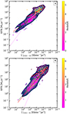Fig. A.1.

SFR vs. $L'_{line}$ $\rm L\prime_{line}$ relations color-coded with respect to redshift.

Appendix B: Total sample

Table B.1 presents our total sample. The individual numbers of sources with [C I](1-0), CO(1-0), CO(2-1) and [C II] are listed along with the total number of sources taken from each sample.

Table B.1.

Used sample of sources.

All Tables

Table 1.

Slope and intercept values for the $M {(H_{2})}^{[C I]}$ $\mathrm M(H_2)^{[CI]}$ vs. $M {(H_{2})}^{CO}$ $\mathrm M(H_2)^{CO}$ relation.

In the text

Table 2.

Slope, intercept, and dispersion values for the SFR (and L_IR in parentheses) vs. $L'_{[CI] ((1 - 0)}$ $\rm L{\prime}_{[CI]((1-0)}$ and $L'_{CO ((1 - 0)}$ $\rm L{\prime}_{CO((1-0)}$ relations.

In the text

Table 3.

Slope, intercept and dispersion values for the SFR vs. $L'_{[CII]}$ $\rm L{\prime}_{[CII]}$ relation.

In the text

Table A.1.

Slope and intercept values for the SFR vs. $L'_{line}$ $\rm L\prime_{line}$ relations.

In the text

Table B.1.

Used sample of sources.

In the text

All Figures

	Fig. 1. Redshift distribution for our sample.
In the text

Fig. 2.

$M {(H_{2})}^{[C I]}$ $\mathrm M(H_2)^{[CI]}$ vs. $M {(H_{2})}^{CO}$ $\mathrm M(H_2)^{CO}$ plot. The best fit using the lmfit package (red dashed line) and the linmix package (thick black solid line) are presented in the figure. The 1-to-1 line is presented as a dashed black line. Finally, the relation derived in Montoya Arroyave et al. (2023) ( $log M {(H_{2})}^{[CI]} = (1.21 \pm 2.42) + (0.91 \pm 0.25) log M {(H_{2})}^{CO}$ $\rm \log M(H_2)^{[CI]} = (1.21 \pm 2.42) + (0.91 \pm 0.25)\,\rm \log M(H_2)^{CO}$ ) is included as a dotted magenta line.

In the text

Fig. 3.

L_IR vs. L′_{[CI](1 − 0)} (panel a), L′_{CO(1 − 0)} (panel b) luminosities, L′_{[CI](1 − 0)}/L′_{CO(1 − 0)} ratio against redshift (panel c), and L′_{[CI](1 − 0)}/L′_{CO(1 − 0)} ratio against L_IR (panel d). The secondary y-axis represents the SFR and the secondary x-axis the total molecular masses computed using the corresponding tracer. We include the best fit using the Levenberg–Marquardt algorithm of the lmfit package (red dashed line), and the Bayesian approach to linear regression using the linmix package (solid black line). In panel (b) we include the relations presented in Sargent et al. (2014) for main-sequence galaxies (thick black dashed line), and starburst galaxies (dash-dotted line). In panels (a) and (b), the relations derived in Montoya Arroyave et al. (2023) for CO(1–0) and [C I](1–0) line detections are presented (magenta dashed lines). Panels (c) and (d) include the lmfit and linmix method fits, with solid red and dashed black lines, respectively. In panel (d), the black dash-dotted line presents the mean L′_{[CI](1 − 0)}/L′_{CO(1 − 0)} value and the scatter (gray shaded area) derived by Gerin & Phillips (2000).

In the text

Fig. 4.

SFR vs. $L'_{[CII]}$ $\rm L{\prime}_{[CII]}$ for the samples of Cormier et al. (2015) (green triangles), Olsen et al. (2017) (orange triangles), Bothwell et al. (2017) (black squares), and Glazer et al. (2024) and references therein (red symbols and teal stars). The red solid line represents the best fit for the listed sample based on a Levenberg–Marquardt algorithm, and the thick black dashed line represents the Bayesian fitting. The gray, black, and blue dashed lines represent different best-fitting relations presented by Herrera-Camus et al. (2015), Pineda et al. (2014), and Sutter et al. (2019), respectively. In addition, we plot with solid black, blue, and green lines the De Looze et al. (2014) Dwarf Galaxy Survey (DGS), and the normal and high star formation efficiency relations by Herrera-Camus et al. (2018) (HC+ 2018), respectively. The relation given in Bisbas et al. (2022) is presented as a dashed magenta line. Finally, the relation that best fits the simulated data presented by Olsen et al. (2017) is included in the figure with a dash-dotted yellow line.

In the text

	Fig. A.1. SFR vs. $L'_{line}$ $\rm L\prime_{line}$ relations color-coded with respect to redshift.
In the text

Current usage metrics show cumulative count of Article Views (full-text article views including HTML views, PDF and ePub downloads, according to the available data) and Abstracts Views on Vision4Press platform.

Data correspond to usage on the plateform after 2015. The current usage metrics is available 48-96 hours after online publication and is updated daily on week days.

Initial download of the metrics may take a while.

[1] Accurso, G., Saintonge, A., Bisbas, T., & Viti, S. 2017, MNRAS, 464, 3315 [NASA ADS] [CrossRef] [Google Scholar]

[2] Alaghband-Zadeh, S., Chapman, S. C., Swinbank, A. M., et al. 2013, MNRAS, 435, 1493 [Google Scholar]

[3] Alatalo, K., Davis, T. A., Bureau, M., et al. 2013, MNRAS, 432, 1796 [NASA ADS] [CrossRef] [Google Scholar]

[4] Alatalo, K., Lisenfeld, U., Lanz, L., et al. 2016, ApJ, 827, 106 [CrossRef] [Google Scholar]

[5] Albrecht, M., Krügel, E., & Chini, R. 2007, A&A, 462, 575 [NASA ADS] [CrossRef] [EDP Sciences] [Google Scholar]

[6] Amodeo, S., Mei, S., Stanford, S. A., et al. 2018, ApJ, 853, 36 [NASA ADS] [CrossRef] [Google Scholar]

[7] Amorín, R., Muñoz-Tuñón, C., Aguerri, J. A. L., & Planesas, P. 2016, A&A, 588, A23 [NASA ADS] [CrossRef] [EDP Sciences] [Google Scholar]

[8] Amvrosiadis, A., Wardlow, J., Birkin, J., et al. 2025, MNRAS, 536, 3757 [Google Scholar]

[9] Andreani, P., Retana-Montenegro, E., Zhang, Z.-Y., et al. 2018, A&A, 615, A142 [NASA ADS] [CrossRef] [EDP Sciences] [Google Scholar]

[10] Ao, Y., Weiß, A., Downes, D., et al. 2008, A&A, 491, 747 [NASA ADS] [CrossRef] [EDP Sciences] [Google Scholar]

[11] Aravena, M., Hodge, J. A., Wagg, J., et al. 2014, MNRAS, 442, 558 [Google Scholar]

[12] Aravena, M., Spilker, J. S., Bethermin, M., et al. 2016, MNRAS, 457, 4406 [Google Scholar]

[13] Astropy Collaboration (Robitaille, T. P., et al.) 2013, A&A, 558, A33 [NASA ADS] [CrossRef] [EDP Sciences] [Google Scholar]

[14] Astropy Collaboration (Price-Whelan, A. M., et al.) 2018, AJ, 156, 123 [Google Scholar]

[15] Astropy Collaboration (Price-Whelan, A. M., et al.) 2022, ApJ, 935, 167 [NASA ADS] [CrossRef] [Google Scholar]

[16] Baan, W. A., Henkel, C., Loenen, A., Baudry, A., & Wiklind, T. 2008, A&A, 477, 747 [NASA ADS] [CrossRef] [EDP Sciences] [Google Scholar]

[17] Bakx, T. J., Eales, S., Negrello, M., et al. 2018, MNRAS, 473, 1751 [NASA ADS] [CrossRef] [Google Scholar]

[18] Bakx, T. J., Tamura, Y., Hashimoto, T., et al. 2020, MNRAS, 493, 4294 [NASA ADS] [CrossRef] [Google Scholar]

[19] Bartelmann, M. 2010, Classical Quantum Gravity, 27, 233001 [NASA ADS] [CrossRef] [Google Scholar]

[20] Bayet, E., Gerin, M., Phillips, T. G., & Contursi, A. 2009, MNRAS, 399, 264 [CrossRef] [Google Scholar]

[21] Berman, D. A., Yun, M. S., Harrington, K., et al. 2022, MNRAS, 515, 3911 [Google Scholar]

[22] Berta, S., Lutz, D., Santini, P., et al. 2013, A&A, 551, A100 [NASA ADS] [CrossRef] [EDP Sciences] [Google Scholar]

[23] Berta, S., Young, A., Cox, P., et al. 2021, A&A, 646, A122 [CrossRef] [EDP Sciences] [Google Scholar]

[24] Berta, S., Stanley, F., Ismail, D., et al. 2023, A&A, 678, A28 [Google Scholar]

[25] Béthermin, M., Greve, T., De Breuck, C., et al. 2018, A&A, 620, A115 [NASA ADS] [CrossRef] [EDP Sciences] [Google Scholar]

[26] Bialy, S., & Sternberg, A. 2015, MNRAS, 450, 4424 [NASA ADS] [CrossRef] [Google Scholar]

[27] Birkin, J. E., Weiss, A., Wardlow, J., et al. 2021, MNRAS, 501, 3926 [CrossRef] [Google Scholar]

[28] Bisbas, T. G., Papadopoulos, P. P., & Viti, S. 2015, ApJ, 803, 37 [NASA ADS] [CrossRef] [Google Scholar]

[29] Bisbas, T. G., Tanaka, K. E., Tan, J. C., Wu, B., & Nakamura, F. 2017a, ApJ, 850, 23 [NASA ADS] [CrossRef] [Google Scholar]

[30] Bisbas, T. G., van Dishoeck, E. F., Papadopoulos, P. P., et al. 2017b, ApJ, 839, 90 [Google Scholar]

[31] Bisbas, T. G., Tan, J. C., & Tanaka, K. E. 2021, MNRAS, 502, 2701 [CrossRef] [Google Scholar]

[32] Bisbas, T. G., Walch, S., Naab, T., et al. 2022, ApJ, 934, 115 [NASA ADS] [CrossRef] [Google Scholar]

[33] Bisbas, T. G., van Dishoeck, E. F., Hu, C.-Y., & Schruba, A. 2023, MNRAS, 519, 729 [Google Scholar]

[34] Bisbas, T. G., Zhang, Z.-Y., Gjergo, E., et al. 2024, MNRAS, 527, 8886 [Google Scholar]

[35] Bisbas, T. G., Zhang, Z.-Y., Kyrmanidou, M.-C., et al. 2025, A&A, 697, A115 [NASA ADS] [CrossRef] [EDP Sciences] [Google Scholar]

[36] Blain, A. W. 1999, MNRAS, 304, 669 [Google Scholar]

[37] Blandford, R. D., & Narayan, R. 1992, ARA&A, 30, 311 [NASA ADS] [CrossRef] [Google Scholar]

[38] Bolatto, A. D., Wolfire, M., & Leroy, A. K. 2013, ARA&A, 51, 207 [CrossRef] [Google Scholar]

[39] Bolatto, A. D., Wong, T., Utomo, D., et al. 2017, ApJ, 846, 159 [Google Scholar]

[40] Boogaard, L. A., van der Werf, P., Weiss, A., et al. 2020, ApJ, 902, 109 [NASA ADS] [CrossRef] [Google Scholar]

[41] Borys, C., Blain, A., Dey, A., et al. 2006, ApJ, 636, 134 [Google Scholar]

[42] Boss, A. P. 2001, ApJ, 551, L167 [Google Scholar]

[43] Bothwell, M., Smail, I., Chapman, S., et al. 2013, MNRAS, 429, 3047 [Google Scholar]

[44] Bothwell, M. S., Aguirre, J. E., Aravena, M., et al. 2017, MNRAS, 466, 2825 [Google Scholar]

[45] Bourne, N., Dunlop, J., Simpson, J., et al. 2019, MNRAS, 482, 3135 [Google Scholar]

[46] Bowler, R., Bourne, N., Dunlop, J., McLure, R., & McLeod, D. 2018, MNRAS, 481, 1631 [Google Scholar]

[47] Boylan-Kolchin, M. 2023, New Astron., 7, 731 [Google Scholar]

[48] Bradač, M., Garcia-Appadoo, D., Huang, K.-H., et al. 2017, ApJ, 836, L2 [Google Scholar]

[49] Brauher, J. R., Dale, D. A., & Helou, G. 2008, ApJS, 178, 280 [NASA ADS] [CrossRef] [Google Scholar]

[50] Burgarella, D., Bogdanoska, J., Nanni, A., et al. 2022, A&A, 664, A73 [NASA ADS] [CrossRef] [EDP Sciences] [Google Scholar]

[51] Bussmann, R., Pérez-Fournon, I., Amber, S., et al. 2013, ApJ, 779, 25 [NASA ADS] [CrossRef] [Google Scholar]

[52] Bussmann, R., Riechers, D., Fialkov, A., et al. 2015, ApJ, 812, 43 [Google Scholar]

[53] Calzetti, D., Kennicutt, R., Engelbracht, C., et al. 2007, ApJ, 666, 870 [NASA ADS] [CrossRef] [Google Scholar]

[54] Cañameras, R., Nesvadba, N., Guery, D., et al. 2015, A&A, 581, A105 [CrossRef] [EDP Sciences] [Google Scholar]

[55] Cañameras, R., Nesvadba, N., Kneissl, R., et al. 2017a, A&A, 600, L3 [NASA ADS] [CrossRef] [EDP Sciences] [Google Scholar]

[56] Cañameras, R., Nesvadba, N., Kneissl, R., et al. 2017b, A&A, 604, A117 [Google Scholar]

[57] Cañameras, R., Yang, C., Nesvadba, N., et al. 2018a, A&A, 620, A61 [NASA ADS] [CrossRef] [EDP Sciences] [Google Scholar]

[58] Cañameras, R., Nesvadba, N., Limousin, M., et al. 2018b, A&A, 620, A60 [NASA ADS] [CrossRef] [EDP Sciences] [Google Scholar]

[59] Cao, Y., Wong, T., Xue, R., et al. 2017, ApJ, 847, 33 [NASA ADS] [CrossRef] [Google Scholar]

[60] Capak, P. L., Carilli, C., Jones, G., et al. 2015, Nature, 522, 455 [NASA ADS] [CrossRef] [Google Scholar]

[61] Carilli, C., Daddi, E., Riechers, D., et al. 2010, ApJ, 714, 1407 [NASA ADS] [CrossRef] [Google Scholar]

[62] Carilli, C., Hodge, J., Walter, F., et al. 2011, ApJ, 739, L33 [NASA ADS] [CrossRef] [Google Scholar]

[63] Carniani, S., Maiolino, R., Amorin, R., et al. 2018, MNRAS, 478, 1170 [NASA ADS] [CrossRef] [Google Scholar]

[64] Carniani, S., Ferrara, A., Maiolino, R., et al. 2020, MNRAS, 499, 5136 [NASA ADS] [CrossRef] [Google Scholar]

[65] Casey, C., Chapman, S., Daddi, E., et al. 2009, MNRAS, 400, 670 [Google Scholar]

[66] Casey, C. M., Narayanan, D., & Cooray, A. 2014, Phys. Rep., 541, 45 [Google Scholar]

[67] Casoli, F., Dickey, J., Kazes, I., et al. 1996, A&AS, 116, 193 [NASA ADS] [CrossRef] [EDP Sciences] [Google Scholar]

[68] Castillo, M. F., Rybak, M., Hodge, J., et al. 2022, ApJ, 930, 35 [NASA ADS] [CrossRef] [Google Scholar]

[69] Castillo, M. F., Hodge, J., Rybak, M., et al. 2023, ApJ, 945, 128 [NASA ADS] [CrossRef] [Google Scholar]

[70] Castillo, M. F., Rybak, M., Hodge, J. A., et al. 2025, ApJ, 987, 158 [Google Scholar]

[71] Chapman, S. C., Blain, A., Smail, I., & Ivison, R. 2005, ApJ, 622, 772 [NASA ADS] [CrossRef] [Google Scholar]

[72] Chapman, S., Ivison, R., Roseboom, I., et al. 2010, MNRAS, 409, L13 [Google Scholar]

[73] Chary, R., & Elbaz, D. 2001, ApJ, 556, 562 [Google Scholar]

[74] Chen, C.-C., Liao, C.-L., Smail, I., et al. 2022, ApJ, 929, 159 [NASA ADS] [CrossRef] [Google Scholar]

[75] Chiang, I. D., Sandstrom, K. M., Chastenet, J., et al. 2024, ApJ, 964, 18 [NASA ADS] [CrossRef] [Google Scholar]

[76] Chu, J. K., Sanders, D., Larson, K., et al. 2017, ApJS, 229, 25 [Google Scholar]

[77] Chung, A., Narayanan, G., Yun, M. S., Heyer, M., & Erickson, N. R. 2009, AJ, 138, 858 [NASA ADS] [CrossRef] [Google Scholar]

[78] Cicone, C., Bothwell, M., Wagg, J., et al. 2017, A&A, 604, A53 [NASA ADS] [CrossRef] [EDP Sciences] [Google Scholar]

[79] Ciesla, L., Béthermin, M., Daddi, E., et al. 2020, A&A, 635, A27 [NASA ADS] [CrossRef] [EDP Sciences] [Google Scholar]

[80] Clark, C. J., Verstocken, S., Bianchi, S., et al. 2018, A&A, 609, A37 [NASA ADS] [CrossRef] [EDP Sciences] [Google Scholar]

[81] Clark, P. C., Glover, S. C., Ragan, S. E., & Duarte-Cabral, A. 2019, MNRAS, 486, 4622 [CrossRef] [Google Scholar]

[82] Cooray, A., Calanog, J., Wardlow, J. L., et al. 2014, ApJ, 790, 40 [NASA ADS] [CrossRef] [Google Scholar]

[83] Coppin, K., Chapin, E. L., Mortier, A. M., et al. 2006, MNRAS, 372, 1621 [Google Scholar]

[84] Cormier, D., Madden, S., Lebouteiller, V., et al. 2015, A&A, 578, A53 [CrossRef] [EDP Sciences] [Google Scholar]

[85] Cortzen, I., Magdis, G. E., Valentino, F., et al. 2020, A&A, 634, L14 [EDP Sciences] [Google Scholar]

[86] Cox, P., Omont, A., Djorgovski, S., et al. 2002, A&A, 387, 406 [NASA ADS] [CrossRef] [EDP Sciences] [Google Scholar]

[87] Cox, P., Krips, M., Neri, R., et al. 2011, ApJ, 740, 63 [NASA ADS] [CrossRef] [Google Scholar]

[88] Cox, P., Neri, R., Berta, S., et al. 2023, A&A, 678, A26 [Google Scholar]

[89] Curran, S., Aalto, S., & Booth, R. 2000, A&AS, 141, 193 [NASA ADS] [CrossRef] [EDP Sciences] [Google Scholar]

[90] Curti, M., Maiolino, R., Curtis-Lake, E., et al. 2024, A&A, 684, A75 [NASA ADS] [CrossRef] [EDP Sciences] [Google Scholar]

[91] Da Cunha, E., Groves, B., Walter, F., et al. 2013, ApJ, 766, 13 [NASA ADS] [CrossRef] [Google Scholar]

[92] da Cunha, E., Walter, F., Smail, I., et al. 2015, ApJ, 806, 110 [NASA ADS] [CrossRef] [Google Scholar]

[93] Daddi, E., Dickinson, M., Morrison, G., et al. 2007, ApJ, 670, 156 [NASA ADS] [CrossRef] [Google Scholar]

[94] Daddi, E., Dannerbauer, H., Stern, D., et al. 2009a, ApJ, 694, 1517 [Google Scholar]

[95] Daddi, E., Dannerbauer, H., Krips, M., et al. 2009b, ApJ, 695, L176 [NASA ADS] [CrossRef] [Google Scholar]

[96] Dale, D. A., Helou, G., Contursi, A., Silbermann, N. A., & Kolhatkar, S. 2001, ApJ, 549, 215 [Google Scholar]

[97] Danielson, A., Swinbank, A., Smail, I., et al. 2011, MNRAS, 410, 1687 [Google Scholar]

[98] Dannerbauer, H., Harrington, K., Díaz-Sánchez, A., et al. 2019, AJ, 158, 34 [Google Scholar]

[99] De Looze, I., Baes, M., Bendo, G. J., Cortese, L., & Fritz, J. 2011, MNRAS, 416, 2712 [Google Scholar]

[100] De Looze, I., Cormier, D., Lebouteiller, V., et al. 2014, A&A, 568, A62 [NASA ADS] [CrossRef] [EDP Sciences] [Google Scholar]

[101] Deane, R., Heywood, I., Rawlings, S., & Marshall, P. 2013, MNRAS, 434, 23 [Google Scholar]

[102] Díaz-Sánchez, A., Iglesias-Groth, S., Rebolo, R., & Dannerbauer, H. 2017, ApJ, 843, L22 [Google Scholar]

[103] Díaz-Santos, T., Armus, L., Charmandaris, V., et al. 2017, ApJ, 846, 32 [Google Scholar]

[104] Dobbs, C. L., Krumholz, M. R., Ballesteros-Paredes, J., et al. 2014, Protostars and Planets VI, 1312, 3 [Google Scholar]

[105] Downes, D., & Solomon, P. 1998, ApJ, 507, 615 [NASA ADS] [CrossRef] [Google Scholar]

[106] Downes, D., & Solomon, P. 2003, ApJ, 582, 37 [NASA ADS] [CrossRef] [Google Scholar]

[107] Downes, D., Solomon, P., & Radford, S. 1995, ApJ, 453, L65 [Google Scholar]

[108] Downes, D., Neri, R., Wiklind, T., Wilner, D., & Shaver, P. 1999, ApJ, 513, L1 [NASA ADS] [CrossRef] [Google Scholar]

[109] Draine, B. T. 2010, Physics of the Interstellar and Intergalactic Medium (Princeton University Press), 19 [Google Scholar]

[110] Draine, B., & Li, A. 2007, ApJ, 657, 810 [NASA ADS] [CrossRef] [Google Scholar]

[111] Drew, P. M., Casey, C. M., Cooray, A., & Whitaker, K. E. 2020, ApJ, 892, 104 [Google Scholar]

[112] Dunne, L., & Eales, S. A. 2001, MNRAS, 327, 697 [Google Scholar]

[113] Dunne, L., Eales, S., Edmunds, M., et al. 2000, MNRAS, 315, 115 [Google Scholar]

[114] Dunne, L., Maddox, S., Vlahakis, C., & Gomez, H. 2021, MNRAS, 501, 2573 [NASA ADS] [CrossRef] [Google Scholar]

[115] Dunne, L., Maddox, S., Papadopoulos, P., Ivison, R., & Gomez, H. 2022, MNRAS, 517, 962 [NASA ADS] [CrossRef] [Google Scholar]

[116] Dye, S., Furlanetto, C., Swinbank, A., et al. 2015, MNRAS, 452, 2258 [NASA ADS] [CrossRef] [Google Scholar]

[117] Elbaz, D., Dickinson, M., Hwang, H. S., et al. 2011, A&A, 533, A119 [NASA ADS] [CrossRef] [EDP Sciences] [Google Scholar]

[118] Emonts, B., Feain, I., Röttgering, H., et al. 2013, MNRAS, 430, 3465 [NASA ADS] [CrossRef] [Google Scholar]

[119] Engel, H., Tacconi, L., Davies, R., et al. 2010, ApJ, 724, 233 [NASA ADS] [CrossRef] [Google Scholar]

[120] Enia, A., Negrello, M., Gurwell, M., et al. 2018, MNRAS, 475, 3467 [Google Scholar]

[121] Falgarone, E., Zwaan, M., Godard, B., et al. 2017, Nature, 548, 430 [NASA ADS] [CrossRef] [Google Scholar]

[122] Feldmann, R., Gnedin, N. Y., & Kravtsov, A. V. 2012, ApJ, 747, 124 [NASA ADS] [CrossRef] [Google Scholar]

[123] Ferrara, A., Vallini, L., Pallottini, A., et al. 2019, MNRAS, 489, 1 [Google Scholar]

[124] Ferrara, A., Sommovigo, L., Dayal, P., et al. 2022, MNRAS, 512, 58 [NASA ADS] [CrossRef] [Google Scholar]

[125] Frayer, D., Ivison, R., Scoville, N., et al. 1999, ApJ, 514, L13 [Google Scholar]

[126] Frayer, D., Harris, A., Baker, A., et al. 2010, ApJ, 726, L22 [Google Scholar]

[127] Frayer, D. T., Maddalena, R. J., Ivison, R., et al. 2018, ApJ, 860, 87 [NASA ADS] [CrossRef] [Google Scholar]

[128] Frye, B. L., Pascale, M., Qin, Y., et al. 2019, ApJ, 871, 51 [NASA ADS] [CrossRef] [Google Scholar]

[129] Fujimoto, S., Oguri, M., Brammer, G., et al. 2021, ApJ, 911, 99 [Google Scholar]

[130] Fujimoto, S., Ouchi, M., Nakajima, K., et al. 2024, ApJ, 964, 146 [NASA ADS] [CrossRef] [Google Scholar]

[131] Gaches, B. A. L., Bisbas, T. G., & Bialy, S. 2022, A&A, 658, A151 [CrossRef] [EDP Sciences] [Google Scholar]

[132] Galametz, M., Madden, S. C., Galliano, F., et al. 2011, A&A, 532, A56 [NASA ADS] [CrossRef] [EDP Sciences] [Google Scholar]

[133] Galametz, M., Kennicutt, R., Calzetti, D., et al. 2013, MNRAS, 431, 1956 [NASA ADS] [CrossRef] [Google Scholar]

[134] Gao, Y., & Solomon, P. M. 2004a, ApJ, 606, 271 [NASA ADS] [CrossRef] [Google Scholar]

[135] Gao, Y., & Solomon, P. M. 2004b, ApJS, 152, 63 [Google Scholar]

[136] García-Burillo, S., Usero, A., Alonso-Herrero, A., et al. 2012, A&A, 539, A8 [Google Scholar]

[137] Gavin, H. P. 2019, Department of Civil and Environmental Engineering, Duke University, 19 [Google Scholar]

[138] Geach, J., More, A., Verma, A., et al. 2015, MNRAS, 452, 502 [NASA ADS] [CrossRef] [Google Scholar]

[139] Geach, J. E., Ivison, R. J., Dye, S., & Oteo, I. 2018, ApJ, 866, L12 [NASA ADS] [CrossRef] [Google Scholar]

[140] Gelman, A. 2004, J. Am. Stat. Assoc., 99, 537 [Google Scholar]

[141] Genzel, R., Baker, A. J., Tacconi, L. J., et al. 2003, ApJ, 584, 633 [NASA ADS] [CrossRef] [Google Scholar]

[142] Genzel, R., Tacconi, L., Combes, F., et al. 2012, ApJ, 746, 69 [Google Scholar]

[143] Gerin, M., & Phillips, T. G. 2000, ApJ, 537, 644 [NASA ADS] [CrossRef] [Google Scholar]

[144] Glazer, K., Bradac, M., Sanders, R. L., et al. 2024, MNRAS, 531, 945 [NASA ADS] [CrossRef] [Google Scholar]

[145] Glover, S. C., & Clark, P. C. 2016, MNRAS, 456, 3596 [NASA ADS] [CrossRef] [Google Scholar]

[146] Gómez-Guijarro, C., Riechers, D., Pavesi, R., et al. 2019, ApJ, 872, 117 [CrossRef] [Google Scholar]

[147] Gong, M., Ostriker, E. C., Kim, C.-G., & Kim, J.-G. 2020, ApJ, 903, 142 [CrossRef] [Google Scholar]

[148] González-López, J., Riechers, D. A., Decarli, R., et al. 2014, ApJ, 784, 99 [Google Scholar]

[149] Graciá-Carpio, J., Sturm, E., Hailey-Dunsheath, S., et al. 2011, ApJ, 728, L7 [Google Scholar]

[150] Grenier, I. A., Black, J. H., & Strong, A. W. 2015, ARA&A, 53, 199 [Google Scholar]

[151] Greve, T. R., Bertoldi, F., Smail, I., et al. 2005, MNRAS, 359, 1165 [NASA ADS] [CrossRef] [Google Scholar]

[152] Greve, T., Leonidaki, I., Xilouris, E., et al. 2014, ApJ, 794, 142 [NASA ADS] [CrossRef] [Google Scholar]

[153] Guilloteau, S., Omont, A., Cox, P., McMahon, R., & Petitjean, P. 1999, A&A, 349, 363 [NASA ADS] [Google Scholar]

[154] Guszejnov, D., & Hopkins, P. F. 2016, MNRAS, 459, 9 [Google Scholar]

[155] Hailey-Dunsheath, S., Sturm, E., Fischer, J., et al. 2012, ApJ, 755, 57 [NASA ADS] [CrossRef] [Google Scholar]

[156] Hainline, L. J., Scoville, N., Yun, M. S., et al. 2004, ApJ, 609, 61 [Google Scholar]

[157] Hainline, L. J., Blain, A., Greve, T., et al. 2006, ApJ, 650, 614 [Google Scholar]

[158] Harikane, Y., Ouchi, M., Inoue, A. K., et al. 2020, ApJ, 896, 93 [Google Scholar]

[159] Harrington, K. C., Yun, M. S., Cybulski, R., et al. 2016, MNRAS, 458, 4383 [NASA ADS] [CrossRef] [Google Scholar]

[160] Harrington, K., Yun, M., Magnelli, B., et al. 2018, MNRAS, 474, 3866 [Google Scholar]

[161] Harrington, K. C., Vishwas, A., Weiß, A., et al. 2019, MNRAS, 488, 1489 [NASA ADS] [CrossRef] [Google Scholar]

[162] Harrington, K. C., Weiss, A., Yun, M. S., et al. 2021, ApJ, 908, 95 [NASA ADS] [CrossRef] [Google Scholar]

[163] Harris, A., Baker, A., Zonak, S., et al. 2010, ApJ, 723, 1139 [NASA ADS] [CrossRef] [Google Scholar]

[164] Hashimoto, T., Laporte, N., Mawatari, K., et al. 2018, Nature, 557, 392 [NASA ADS] [CrossRef] [Google Scholar]

[165] Hashimoto, T., Inoue, A. K., Mawatari, K., et al. 2019, PASJ, 71, 71 [Google Scholar]

[166] Heintz, K. E., & Watson, D. 2020, ApJ, 889, L7 [Google Scholar]

[167] Heintz, K., Giménez-Arteaga, C., Fujimoto, S., et al. 2023, ApJ, 944, L30 [NASA ADS] [CrossRef] [Google Scholar]

[168] Hennebelle, P., & Grudić, M. Y. 2024, ARA&A, 62, 63 [Google Scholar]

[169] Herrera-Camus, R., Bolatto, A., Wolfire, M., et al. 2015, ApJ, 800, 1 [Google Scholar]

[170] Herrera-Camus, R., Sturm, E., Graciá-Carpio, J., et al. 2018, ApJ, 861, 95 [Google Scholar]

[171] Herrero-Illana, R., Privon, G., Evans, A. S., et al. 2019, A&A, 628, A71 [NASA ADS] [CrossRef] [EDP Sciences] [Google Scholar]

[172] Hezaveh, Y. D., Marrone, D. P., & Holder, G. P. 2012, ApJ, 761, 20 [NASA ADS] [CrossRef] [Google Scholar]

[173] Hill, R., Chapman, S. C., Scott, D., et al. 2018, MNRAS, 477, 2042 [Google Scholar]

[174] Hodge, J., Riechers, D., Decarli, R., et al. 2014, ApJ, 798, L18 [NASA ADS] [CrossRef] [Google Scholar]

[175] Hopkins, P. F., Younger, J. D., Hayward, C. C., Narayanan, D., & Hernquist, L. 2010, MNRAS, 402, 1693 [NASA ADS] [CrossRef] [Google Scholar]

[176] Hughes, T., Ibar, E., Villanueva, V., et al. 2017, MNRAS, 468, L103 [NASA ADS] [CrossRef] [Google Scholar]

[177] Hunt, L. K., De Looze, I., Boquien, M., et al. 2019, A&A, 621, A51 [NASA ADS] [CrossRef] [EDP Sciences] [Google Scholar]

[178] Hunter, D. A., Elmegreen, B. G., & Madden, S. C. 2024, ARA&A, 62, 113 [NASA ADS] [CrossRef] [Google Scholar]

[179] Huynh, M. T., Emonts, B., Kimball, A., et al. 2017, MNRAS, 467, 1222 [Google Scholar]

[180] Iglesias-Groth, S., Díaz-Sánchez, A., Rebolo, R., & Dannerbauer, H. 2017, MNRAS, 467, 330 [Google Scholar]

[181] Ikeda, M., Oka, T., Tatematsu, K., Sekimoto, Y., & Yamamoto, S. 2002, ApJS, 139, 467 [NASA ADS] [CrossRef] [Google Scholar]

[182] Inoue, A. K., Tamura, Y., Matsuo, H., et al. 2016, Science, 352, 1559 [NASA ADS] [CrossRef] [Google Scholar]

[183] Inutsuka, S.-I., Inoue, T., Iwasaki, K., & Hosokawa, T. 2015, A&A, 580, A49 [NASA ADS] [CrossRef] [EDP Sciences] [Google Scholar]

[184] Iono, D., Wilson, C. D., Yun, M. S., et al. 2009, ApJ, 695, 1537 [NASA ADS] [CrossRef] [Google Scholar]

[185] Iono, D., Hatsukade, B., Kohno, K., et al. 2012, PASJ, 64, L2 [NASA ADS] [Google Scholar]

[186] Ismail, D., Beelen, A., Buat, V., et al. 2023, A&A, 678, A27 [Google Scholar]

[187] Ivison, R., Swinbank, A., Swinyard, B., et al. 2010, A&A, 518, L35 [NASA ADS] [CrossRef] [EDP Sciences] [Google Scholar]

[188] Ivison, R., Papadopoulos, P., Smail, I., et al. 2011, MNRAS, 412, 1913 [Google Scholar]

[189] Ivison, R., Swinbank, A., Smail, I., et al. 2013, ApJ, 772, 137 [NASA ADS] [CrossRef] [Google Scholar]

[190] Izumi, T., Nguyen, D. D., Imanishi, M., et al. 2020, ApJ, 898, 75 [NASA ADS] [CrossRef] [Google Scholar]

[191] Jarugula, S., Vieira, J. D., Weiss, A., et al. 2021, ApJ, 921, 97 [NASA ADS] [CrossRef] [Google Scholar]

[192] Jiao, Q., Zhao, Y., Zhu, M., et al. 2017, ApJ, 840, L18 [Google Scholar]

[193] Jiao, Q., Zhao, Y., Lu, N., et al. 2019, ApJ, 880, 133 [Google Scholar]

[194] Jiao, Q., Gao, Y., & Zhao, Y. 2021, MNRAS, 504, 2360 [NASA ADS] [CrossRef] [Google Scholar]

[195] Jin, S., Daddi, E., Magdis, G., et al. 2019, ApJ, 887, 144 [Google Scholar]

[196] Jo, J. U., Youn, S., Kim, S., et al. 2021, Ap&SS, 366, 18 [Google Scholar]

[197] Juneau, S., Narayanan, D., Moustakas, J., et al. 2009, ApJ, 707, 1217 [NASA ADS] [CrossRef] [Google Scholar]

[198] Kaasinen, M., Scoville, N., Walter, F., et al. 2019, ApJ, 880, 15 [NASA ADS] [CrossRef] [Google Scholar]

[199] Kamenetzky, J., Rangwala, N., Glenn, J., Maloney, P., & Conley, A. 2016a, VizieR Online Data Catalog: J/ApJ/829/93 [Google Scholar]

[200] Kamenetzky, J., Rangwala, N., Glenn, J., Maloney, P., & Conley, A. 2016b, ApJ, 829, 93 [NASA ADS] [CrossRef] [Google Scholar]

[201] Kamieneski, P. S., Yun, M. S., Harrington, K. C., et al. 2024, ApJ, 961, 2 [NASA ADS] [CrossRef] [Google Scholar]

[202] Kanekar, N., Wagg, J., Chary, R. R., & Carilli, C. L. 2013, ApJ, 771, L20 [NASA ADS] [CrossRef] [Google Scholar]

[203] Katz, H., Kimm, T., Sijacki, D., & Haehnelt, M. G. 2017, MNRAS, 468, 4831 [Google Scholar]

[204] Kelly, B. C. 2007, ApJ, 665, 1489 [Google Scholar]

[205] Kennicutt, R. C. 1998a, ARA&A, 36, 189 [NASA ADS] [CrossRef] [Google Scholar]

[206] Kennicutt, R. C. 1998b, ApJ, 498, 541 [NASA ADS] [CrossRef] [Google Scholar]

[207] Kennicutt, R. C., & Evans, N. J. 2012, ARA&A, 50, 531 [NASA ADS] [CrossRef] [Google Scholar]

[208] Khatri, R., & Gaspari, M. 2016, MNRAS, 463, 655 [Google Scholar]

[209] Khusanova, Y., Bethermin, M., Le Fèvre, O., et al. 2021, A&A, 649, A152 [NASA ADS] [CrossRef] [EDP Sciences] [Google Scholar]

[210] Kneib, J.-P., Neri, R., Smail, I., et al. 2005, A&A, 434, 819 [NASA ADS] [CrossRef] [EDP Sciences] [Google Scholar]

[211] Knudsen, K. K., Richard, J., Kneib, J.-P., et al. 2016, MNRAS, 462, L6 [NASA ADS] [CrossRef] [Google Scholar]

[212] Knudsen, K. K., Watson, D., Frayer, D., et al. 2017, MNRAS, 466, 138 [NASA ADS] [CrossRef] [Google Scholar]

[213] Koda, J., Sawada, T., Wright, M. C., et al. 2011, ApJS, 193, 19 [NASA ADS] [CrossRef] [Google Scholar]

[214] Kovacs, A., Chapman, S., Dowell, C., et al. 2006, ApJ, 650, 592 [CrossRef] [Google Scholar]

[215] Kuno, N., Sato, N., Nakanishi, H., et al. 2007, PASJ, 59, 117 [NASA ADS] [Google Scholar]

[216] Lada, E. A., & Blitz, L. 1988, ApJ, 326, L69 [Google Scholar]

[217] Lagache, G., Cousin, M., & Chatzikos, M. 2018, A&A, 609, A130 [NASA ADS] [CrossRef] [EDP Sciences] [Google Scholar]

[218] Lahén, N., Naab, T., & Kauffmann, G. 2022, MNRAS, 514, 4560 [CrossRef] [Google Scholar]

[219] Langer, W. D., Velusamy, T., Pineda, J. L., Willacy, K., & Goldsmith, P. F. 2014, A&A, 561, A122 [NASA ADS] [CrossRef] [EDP Sciences] [Google Scholar]

[220] Lapham, R. C., & Young, L. M. 2019, ApJ, 875, 3 [NASA ADS] [CrossRef] [Google Scholar]

[221] Larson, R. B. 1973, ARA&A, 11, 219 [NASA ADS] [CrossRef] [Google Scholar]

[222] Le Floc’h, E., Papovich, C., Dole, H., et al. 2005, ApJ, 632, 169 [Google Scholar]

[223] Leroy, A., Bolatto, A., Simon, J., & Blitz, L. 2005, ApJ, 625, 763 [NASA ADS] [CrossRef] [Google Scholar]

[224] Leroy, A. K., Bolatto, A., Gordon, K., et al. 2011, ApJ, 737, 12 [Google Scholar]

[225] Lestrade, J.-F., Carilli, C. L., Thanjavur, K., et al. 2011, ApJ, 739, L30 [NASA ADS] [CrossRef] [Google Scholar]

[226] Leung, T. D., Riechers, D. A., Baker, A. J., et al. 2019, ApJ, 871, 85 [NASA ADS] [CrossRef] [Google Scholar]

[227] Liang, L., Feldmann, R., Murray, N., et al. 2023, MNRAS, 528, 499 [Google Scholar]

[228] Liao, C.-L., Chen, C.-C., Wang, W.-H., et al. 2024, ApJ, 961, 226 [NASA ADS] [CrossRef] [Google Scholar]

[229] Lisenfeld, U., Espada, D., Verdes-Montenegro, L., et al. 2011, A&A, 534, A102 [NASA ADS] [CrossRef] [EDP Sciences] [Google Scholar]

[230] Liu, D., Gao, Y., Isaak, K., et al. 2015, ApJ, 810, L14 [NASA ADS] [CrossRef] [Google Scholar]

[231] Lo, N., Cunningham, M., Jones, P., et al. 2014, ApJ, 797, L17 [NASA ADS] [CrossRef] [Google Scholar]

[232] Lu, N., Zhao, Y., Díaz-Santos, T., et al. 2017, ApJS, 230, 1 [Google Scholar]

[233] Luo, G., Zhang, Z.-Y., Bisbas, T. G., et al. 2023, ApJ, 942, 101 [NASA ADS] [CrossRef] [Google Scholar]

[234] Madden, S., Rémy-Ruyer, A., Galametz, M., et al. 2013, PASP, 125, 600 [NASA ADS] [CrossRef] [Google Scholar]

[235] Madden, S., Cormier, D., Hony, S., et al. 2020, A&A, 643, A141 [NASA ADS] [CrossRef] [EDP Sciences] [Google Scholar]

[236] Magdis, G. E., Daddi, E., Elbaz, D., et al. 2011, ApJ, 740, L15 [NASA ADS] [CrossRef] [Google Scholar]

[237] Magnelli, B., Elbaz, D., Chary, R., et al. 2009, A&A, 496, 57 [NASA ADS] [CrossRef] [EDP Sciences] [Google Scholar]

[238] Magnelli, B., Elbaz, D., Chary, R., et al. 2011, A&A, 528, A35 [NASA ADS] [CrossRef] [EDP Sciences] [Google Scholar]

[239] Magnelli, B., Lutz, D., Santini, P., et al. 2012, A&A, 539, A155 [NASA ADS] [CrossRef] [EDP Sciences] [Google Scholar]

[240] Maiolino, R., Carniani, S., Fontana, A., et al. 2015, MNRAS, 452, 54 [NASA ADS] [CrossRef] [Google Scholar]

[241] Matthee, J., Sobral, D., Boone, F., et al. 2017, ApJ, 851, 145 [NASA ADS] [CrossRef] [Google Scholar]

[242] Matthee, J., Sobral, D., Boogaard, L. A., et al. 2019, ApJ, 881, 124 [NASA ADS] [CrossRef] [Google Scholar]

[243] McKean, J., Berciano Alba, A., Volino, F., et al. 2011, MNRAS, 414, L11 [Google Scholar]

[244] McKee, C. F., & Ostriker, E. C. 2007, ARA&A, 45, 565 [Google Scholar]

[245] Messias, H., Dye, S., Nagar, N., et al. 2014, A&A, 568, A92 [NASA ADS] [CrossRef] [EDP Sciences] [Google Scholar]

[246] Messias, H., Nagar, N., Zhang, Z.-Y., et al. 2019, MNRAS, 486, 2366 [Google Scholar]

[247] Michiyama, T., Ueda, J., Tadaki, K.-I., et al. 2020, ApJ, 897, L19 [NASA ADS] [CrossRef] [Google Scholar]

[248] Mirabel, I., Booth, R., Garay, G., Johansson, L., & Sanders, D. 1990, A&A, 236, 327 [Google Scholar]

[249] Molyneux, S., Smit, R., Schaerer, D., et al. 2022, MNRAS, 512, 535 [Google Scholar]

[250] Montoya Arroyave, I., Cicone, C., Makroleivaditi, E., et al. 2023, A&A, 673, A13 [NASA ADS] [CrossRef] [EDP Sciences] [Google Scholar]

[251] Narayanan, D., & Krumholz, M. R. 2014, MNRAS, 442, 1411 [NASA ADS] [CrossRef] [Google Scholar]

[252] Nayyeri, H., Keele, M., Cooray, A., et al. 2016, ApJ, 823, 17 [NASA ADS] [CrossRef] [Google Scholar]

[253] Negrello, M., Hopwood, R., Dye, S., et al. 2014, MNRAS, 440, 1999 [NASA ADS] [CrossRef] [Google Scholar]

[254] Negrello, M., Amber, S., Amvrosiadis, A., et al. 2017, MNRAS, 465, 3558 [NASA ADS] [CrossRef] [Google Scholar]

[255] Neri, R., Genzel, R., Ivison, R., et al. 2003, ApJ, 597, L113 [Google Scholar]

[256] Neri, R., Cox, P., Omont, A., et al. 2020, A&A, 635, A7 [NASA ADS] [CrossRef] [EDP Sciences] [Google Scholar]

[257] Nesvadba, N., Cañameras, R., Kneissl, R., et al. 2019, A&A, 624, A23 [NASA ADS] [CrossRef] [EDP Sciences] [Google Scholar]

[258] Offner, S. S., Bisbas, T. G., Bell, T. A., & Viti, S. 2014, MNRAS, 440, L81 [NASA ADS] [CrossRef] [Google Scholar]

[259] Olsen, K., Greve, T. R., Narayanan, D., et al. 2017, ApJ, 846, 105 [Google Scholar]

[260] Ossenkopf, V., Rollig, M., Cubick, M., & Stutzki, J. 2007, Molecules in Space and Laboratory, 95 [Google Scholar]

[261] Ota, K., Walter, F., Ohta, K., et al. 2014, ApJ, 792, 34 [NASA ADS] [CrossRef] [Google Scholar]

[262] Oteo, I., Zhang, Z., Yang, C., et al. 2017, ApJ, 850, 170 [NASA ADS] [CrossRef] [Google Scholar]

[263] Oteo, I., Ivison, R., Dunne, L., et al. 2018, ApJ, 856, 72 [Google Scholar]

[264] Ouchi, M., Ellis, R., Ono, Y., et al. 2013, ApJ, 778, 102 [NASA ADS] [CrossRef] [Google Scholar]

[265] Padovani, M., Galli, D., & Glassgold, A. E. 2009, A&A, 501, 619 [NASA ADS] [CrossRef] [EDP Sciences] [Google Scholar]

[266] Papadopoulos, P. P. 2010, ApJ, 720, 226 [NASA ADS] [CrossRef] [Google Scholar]

[267] Papadopoulos, P. P., & Greve, T. R. 2004, ApJ, 615, L29 [Google Scholar]

[268] Papadopoulos, P. P., Thi, W.-F., & Viti, S. 2004, MNRAS, 351, 147 [Google Scholar]

[269] Papadopoulos, P. P., van der Werf, P. P., Xilouris, E., et al. 2012, MNRAS, 426, 2601 [NASA ADS] [CrossRef] [Google Scholar]

[270] Papadopoulos, P. P., Bisbas, T. G., & Zhang, Z.-Y. 2018, MNRAS, 478, 1716 [NASA ADS] [CrossRef] [Google Scholar]

[271] Papadopoulos, P., Dunne, L., & Maddox, S. 2022, MNRAS, 510, 725 [Google Scholar]

[272] Pappalardo, C., Bianchi, S., Corbelli, E., et al. 2012, A&A, 545, A75 [NASA ADS] [CrossRef] [EDP Sciences] [Google Scholar]

[273] Pavesi, R., Riechers, D. A., Sharon, C. E., et al. 2018a, ApJ, 861, 43 [Google Scholar]

[274] Pavesi, R., Sharon, C. E., Riechers, D. A., et al. 2018b, ApJ, 864, 49 [Google Scholar]

[275] Pentericci, L., Carniani, S., Castellano, M., et al. 2016, ApJ, 829, L11 [NASA ADS] [CrossRef] [Google Scholar]

[276] Pereira-Santaella, M., Spinoglio, L., Busquet, G., et al. 2013, ApJ, 768, 55 [Google Scholar]

[277] Pérez-Beaupuits, J., Stutzki, J., Ossenkopf, V., et al. 2015a, A&A, 575, A9 [NASA ADS] [CrossRef] [EDP Sciences] [Google Scholar]

[278] Pérez-Beaupuits, J. P., Güsten, R., Spaans, M., et al. 2015b, A&A, 583, A107 [NASA ADS] [CrossRef] [EDP Sciences] [Google Scholar]

[279] Perna, M., Sargent, M., Brusa, M., et al. 2018, A&A, 619, A90 [NASA ADS] [CrossRef] [EDP Sciences] [Google Scholar]

[280] Pilbratt, G., Riedinger, J., Passvogel, T., et al. 2010, A&A, 518, L1 [NASA ADS] [CrossRef] [EDP Sciences] [Google Scholar]

[281] Pineda, J., Langer, W., & Goldsmith, P. 2014, A&A, 570, A121 [NASA ADS] [CrossRef] [EDP Sciences] [Google Scholar]

[282] Planck Collaboration XVI. 2014, A&A, 571, A16 [NASA ADS] [CrossRef] [EDP Sciences] [Google Scholar]

[283] Popping, G., Decarli, R., Man, A. W., et al. 2017, A&A, 602, A11 [NASA ADS] [CrossRef] [EDP Sciences] [Google Scholar]

[284] Ramambason, L., Lebouteiller, V., Madden, S., et al. 2024, A&A, 681, A14 [NASA ADS] [CrossRef] [EDP Sciences] [Google Scholar]

[285] Ramos Padilla, A. F., Wang, L., Ploeckinger, S., van der Tak, F. F. S., & Trager, S. C. 2021, A&A, 645, A133 [NASA ADS] [CrossRef] [EDP Sciences] [Google Scholar]

[286] Riechers, D. A., Carilli, C. L., Maddalena, R. J., et al. 2011a, ApJ, 739, L32 [CrossRef] [Google Scholar]

[287] Riechers, D. A., Carilli, L. C., Walter, F., et al. 2011b, ApJ, 733, L11 [Google Scholar]

[288] Riechers, D. A., Hodge, J., Walter, F., Carilli, C. L., & Bertoldi, F. 2011c, ApJ, 739, L31 [Google Scholar]

[289] Riechers, D. A., Bradford, C., Clements, D., et al. 2013, Nature, 496, 329 [CrossRef] [Google Scholar]

[290] Riechers, D. A., Hodge, J. A., Pavesi, R., et al. 2020a, ApJ, 895, 81 [Google Scholar]

[291] Riechers, D. A., Boogaard, L. A., Decarli, R., et al. 2020b, ApJ, 896, L21 [NASA ADS] [CrossRef] [Google Scholar]

[292] Rivera, J., Baker, A. J., Gallardo, P. A., et al. 2019, ApJ, 879, 95 [NASA ADS] [CrossRef] [Google Scholar]

[293] Rosenberg, M., Van Der Werf, P., Aalto, S., et al. 2015, ApJ, 801, 72 [Google Scholar]

[294] Salpeter, E. E. 1955, ApJ, 121, 161 [Google Scholar]

[295] Sandstrom, K. M., Leroy, A., Walter, F., et al. 2013, ApJ, 777, 5 [NASA ADS] [CrossRef] [Google Scholar]

[296] Sargent, M. T., Daddi, E., Béthermin, M., et al. 2014, ApJ, 793, 19 [NASA ADS] [CrossRef] [Google Scholar]

[297] Sargsyan, L., Lebouteiller, V., Weedman, D., et al. 2012, ApJ, 755, 171 [Google Scholar]

[298] Schaerer, D., Boone, F., Zamojski, M., et al. 2015, A&A, 574, A19 [NASA ADS] [CrossRef] [EDP Sciences] [Google Scholar]

[299] Schmidt, M. 1959, ApJ, 129, 243 [NASA ADS] [CrossRef] [Google Scholar]

[300] Schouws, S., Bouwens, R., Smit, R., et al. 2023, ApJ, 954, 103 [NASA ADS] [CrossRef] [Google Scholar]

[301] Schruba, A., Leroy, A. K., Walter, F., et al. 2012, AJ, 143, 138 [NASA ADS] [CrossRef] [Google Scholar]

[302] Schruba, A., Leroy, A. K., Kruijssen, J. D., et al. 2017, ApJ, 835, 278 [NASA ADS] [CrossRef] [Google Scholar]

[303] Scoville, N., Sheth, K., Aussel, H., et al. 2016, ApJ, 820, 83 [Google Scholar]

[304] Seifried, D., Haid, S., Walch, S., Borchert, E. M. A., & Bisbas, T. G. 2020, MNRAS, 492, 1465 [NASA ADS] [CrossRef] [Google Scholar]

[305] Serjeant, S. 2012, MNRAS, 424, 2429 [NASA ADS] [CrossRef] [Google Scholar]

[306] Serjeant, S., Geach, J., Dunlop, J., et al. 2017, MNRAS, 465, 1789 [NASA ADS] [CrossRef] [Google Scholar]

[307] Sharon, C. E., Baker, A. J., Harris, A. I., & Thomson, A. P. 2013, ApJ, 765, 6 [NASA ADS] [CrossRef] [Google Scholar]

[308] Sharon, C. E., Riechers, D. A., Hodge, J., et al. 2016, ApJ, 827, 18 [Google Scholar]

[309] Sheth, K., Blain, A. W., Kneib, J.-P., et al. 2004, ApJ, 614, L5 [Google Scholar]

[310] Shi, Y., Wang, J., Zhang, Z.-Y., et al. 2016, Nat. Commun., 7, 13789 [NASA ADS] [CrossRef] [Google Scholar]

[311] Simpson, J., Smail, I., Swinbank, A., et al. 2015, ApJ, 807, 128 [Google Scholar]

[312] Simpson, J., Smail, I., Swinbank, A., et al. 2019, ApJ, 880, 43 [NASA ADS] [CrossRef] [Google Scholar]

[313] Simpson, J., Smail, I., Dudzevičiūtė, U., et al. 2020, MNRAS, 495, 3409 [NASA ADS] [CrossRef] [Google Scholar]

[314] Smit, R., Bouwens, R. J., Carniani, S., et al. 2018, Nature, 553, 178 [Google Scholar]

[315] Sneppen, A., Steinhardt, C. L., Hensley, H., et al. 2022, ApJ, 931, 57 [NASA ADS] [CrossRef] [Google Scholar]

[316] Solomon, P. M., & Vanden Bout, P. A. 2005, ARA&A, 43, 677 [NASA ADS] [CrossRef] [Google Scholar]

[317] Solomon, P. M., Downes, D., Radford, S. J. E., & Barrett, J. W. 1997, ApJ, 478, 144 [NASA ADS] [CrossRef] [Google Scholar]

[318] Sommovigo, L., Ferrara, A., Pallottini, A., et al. 2022, MNRAS, 513, 3122 [NASA ADS] [CrossRef] [Google Scholar]

[319] Sorai, K., Kuno, N., Muraoka, K., et al. 2019, PASJ, 71, S14 [Google Scholar]

[320] Spilker, J., Marrone, D. P., Aravena, M., et al. 2016, ApJ, 826, 112 [NASA ADS] [CrossRef] [Google Scholar]

[321] Spoon, H. W., Farrah, D., Lebouteiller, V., et al. 2013, ApJ, 775, 127 [NASA ADS] [CrossRef] [Google Scholar]

[322] Stacey, G., Hailey-Dunsheath, S., Ferkinhoff, C., et al. 2010, ApJ, 724, 957 [NASA ADS] [CrossRef] [Google Scholar]

[323] Stacey, H., McKean, J., Powell, D., et al. 2021, MNRAS, 500, 3667 [Google Scholar]

[324] Stach, S. M., Smail, I., Swinbank, A., et al. 2018, ApJ, 860, 161 [Google Scholar]

[325] Steinhardt, C. L., Kokorev, V., Rusakov, V., Garcia, E., & Sneppen, A. 2023, ApJ, 951, L40 [NASA ADS] [CrossRef] [Google Scholar]

[326] Stevens, J. A., Amure, M., & Gear, W. K. 2005, MNRAS, 357, 361 [Google Scholar]

[327] Strong, A. W., Moskalenko, I. V., & Ptuskin, V. S. 2007, Annu. Rev. Nucl. Part. Sci., 57, 285 [NASA ADS] [CrossRef] [Google Scholar]

[328] Sturm, E., Verma, A., Graciá-Carpio, J., et al. 2010, A&A, 518, L36 [NASA ADS] [CrossRef] [EDP Sciences] [Google Scholar]

[329] Sturm, E., González-Alfonso, E., Veilleux, S., et al. 2011, ApJ, 733, L16 [NASA ADS] [CrossRef] [Google Scholar]

[330] Su, T., Marriage, T. A., Asboth, V., et al. 2017, MNRAS, 464, 968 [Google Scholar]

[331] Sutter, J., Dale, D. A., Croxall, K. V., et al. 2019, ApJ, 886, 60 [NASA ADS] [CrossRef] [Google Scholar]

[332] Swinbank, A., Simpson, J., Smail, I., et al. 2014, MNRAS, 438, 1267 [Google Scholar]

[333] Tacconi, L. J., Neri, R., Chapman, S., et al. 2006, ApJ, 640, 228 [NASA ADS] [CrossRef] [Google Scholar]

[334] Talia, M., Pozzi, F., Vallini, L., et al. 2018, MNRAS, 476, 3956 [NASA ADS] [CrossRef] [Google Scholar]

[335] Tan, Q., Daddi, E., Magdis, G., et al. 2014, A&A, 569, A98 [NASA ADS] [CrossRef] [EDP Sciences] [Google Scholar]

[336] Teng, Y.-H., Sandstrom, K. M., Sun, J., et al. 2022, ApJ, 925, 72 [NASA ADS] [CrossRef] [Google Scholar]

[337] Thomas, H., Dunne, L., Green, D., et al. 2004, MNRAS, 348, 1197 [Google Scholar]

[338] Thomson, A., Ivison, R., Smail, I., et al. 2012, MNRAS, 425, 2203 [NASA ADS] [CrossRef] [Google Scholar]

[339] Tinney, C., Scoville, N., Sanders, D., & Soifer, B. 1990, ApJ, 362, 473 [Google Scholar]

[340] Tinsley, B. M. 1968, ApJ, 151, 547 [Google Scholar]

[341] Tinsley, B. M. 1972, A&A, 20, 383 [NASA ADS] [Google Scholar]

[342] Ueda, J., Iono, D., Yun, M. S., et al. 2014, ApJS, 214, 1 [Google Scholar]

[343] Valentino, F., Magdis, G. E., Daddi, E., et al. 2018, ApJ, 869, 27 [Google Scholar]

[344] Valentino, F., Magdis, G. E., Daddi, E., et al. 2020, ApJ, 890, 24 [Google Scholar]

[345] Valentino, F., Brammer, G., Fujimoto, S., et al. 2022, ApJ, 929, L9 [NASA ADS] [CrossRef] [Google Scholar]

[346] Vallini, L., Gallerani, S., Ferrara, A., Pallottini, A., & Yue, B. 2015, ApJ, 813, 36 [NASA ADS] [CrossRef] [Google Scholar]

[347] van Dishoeck, E. F. 1990, in The Evolution of the Interstellar Medium, ed. L. Blitz, ASP Conf. Ser., 12, 207 [Google Scholar]

[348] van Dishoeck, E. F. 1992, in Astrochemistry of Cosmic Phenomena, ed. P. D. Singh, 150, 143 [Google Scholar]

[349] Veilleux, S., Meléndez, M., Sturm, E., et al. 2013, ApJ, 776, 27 [Google Scholar]

[350] Velusamy, T., & Langer, W. 2014, A&A, 572, A45 [NASA ADS] [CrossRef] [EDP Sciences] [Google Scholar]

[351] Villanueva, V., Ibar, E., Hughes, T., et al. 2017, MNRAS, 470, 3775 [NASA ADS] [CrossRef] [Google Scholar]

[352] Walter, F., Weiss, A., Downes, D., Decarli, R., & Henkel, C. 2011, ApJ, 730, 18 [NASA ADS] [CrossRef] [Google Scholar]

[353] Walter, F., Decarli, R., Carilli, C., et al. 2012, Nature, 486, 233 [Google Scholar]

[354] Wang, T., Elbaz, D., Daddi, E., et al. 2018, ApJ, 867, L29 [NASA ADS] [CrossRef] [Google Scholar]

[355] Wang, T., Schreiber, C., Elbaz, D., et al. 2019, Nature, 572, 211 [Google Scholar]

[356] Watson, D., Christensen, L., Knudsen, K. K., et al. 2015, Nature, 519, 327 [Google Scholar]

[357] Weiß, A., Henkel, C., Downes, D., & Walter, F. 2003, A&A, 409, L41 [NASA ADS] [CrossRef] [EDP Sciences] [Google Scholar]

[358] Weiß, A., Downes, D., Henkel, C., & Walter, F. 2005, A&A, 429, L25 [NASA ADS] [CrossRef] [EDP Sciences] [Google Scholar]

[359] Weiß, A., De Breuck, C., Marrone, D., et al. 2013, ApJ, 767, 88 [CrossRef] [Google Scholar]

[360] White, G. J., Ellison, B., Claude, S., Dent, W. R. F., & Matheson, D. N. 1994, A&A, 284, L23 [NASA ADS] [Google Scholar]

[361] Willott, C. J., Carilli, C. L., Wagg, J., & Wang, R. 2015, ApJ, 807, 180 [NASA ADS] [CrossRef] [Google Scholar]

[362] Wilson, C. D., Petitpas, G. R., Iono, D., et al. 2008, ApJS, 178, 189 [Google Scholar]

[363] Wong, T., Xue, R., Bolatto, A. D., et al. 2013, ApJ, 777, L4 [NASA ADS] [CrossRef] [Google Scholar]

[364] Wong, K. C., Ishida, T., Tamura, Y., et al. 2017, ApJ, 843, L35 [Google Scholar]

[365] Wong, Y. H. V., Wang, P., Hashimoto, T., et al. 2022, ApJ, 929, 161 [NASA ADS] [CrossRef] [Google Scholar]

[366] Wu, J., Evans, N. J., II, Gao, Y., et al. 2005, ApJ, 635, L173 [NASA ADS] [CrossRef] [Google Scholar]

[367] Wu, J., Bout, P. A. V., Evans, N. J., & Dunham, M. M. 2009, ApJ, 707, 988 [NASA ADS] [CrossRef] [Google Scholar]

[368] Wu, B., Tan, J. C., Nakamura, F., et al. 2017, ApJ, 835, 137 [NASA ADS] [CrossRef] [Google Scholar]

[369] Yamashita, T., Komugi, S., Matsuhara, H., et al. 2017, ApJ, 844, 96 [Google Scholar]

[370] Yang, C., Omont, A., Beelen, A., et al. 2017, A&A, 608, A144 [NASA ADS] [CrossRef] [EDP Sciences] [Google Scholar]

[371] Yang, C., Gavazzi, R., Beelen, A., et al. 2019, A&A, 624, A138 [NASA ADS] [CrossRef] [EDP Sciences] [Google Scholar]

[372] Yao, L., Seaquist, E., Kuno, N., & Dunne, L. 2003, ApJ, 588, 771 [NASA ADS] [CrossRef] [Google Scholar]

[373] Young, J. S., Xie, S., Tacconi, L., et al. 1995, ApJS, 98, 219 [NASA ADS] [CrossRef] [Google Scholar]

[374] Young, L. M., Bureau, M., & Cappellari, M. 2008, ApJ, 676, 317 [NASA ADS] [CrossRef] [Google Scholar]

[375] Zanella, A., Daddi, E., Magdis, G., et al. 2018, MNRAS, 481, 1976 [Google Scholar]

[376] Zhang, Z.-Y., Gao, Y., Henkel, C., et al. 2014a, ApJ, 784, L31 [NASA ADS] [CrossRef] [Google Scholar]

[377] Zhang, Z.-Y., Henkel, C., Gao, Y., et al. 2014b, A&A, 568, A122 [NASA ADS] [CrossRef] [EDP Sciences] [Google Scholar]

[378] Zhang, Z.-Y., Papadopoulos, P. P., Ivison, R., et al. 2016, R. Soc. Open Sci., 3, 160025 [NASA ADS] [CrossRef] [Google Scholar]

[379] Zhang, Z.-Y., Romano, D., Ivison, R., Papadopoulos, P. P., & Matteucci, F. 2018, Nature, 558, 260 [NASA ADS] [CrossRef] [Google Scholar]

[380] Zhou, J., Zhang, Z.-Y., Gao, Y., et al. 2022, ApJ, 936, 58 [NASA ADS] [CrossRef] [Google Scholar]

[381] Zhu, M., Seaquist, E., Davoust, E., Frayer, D. T., & Bushouse, H. A. 1999, AJ, 118, 145 [Google Scholar]

Tight correlation of star formation with [CI] and CO lines across cosmic time

1. Introduction

2. Sample selection

3. Results and analysis

3.1. Magnification corrections

3.2. Regression models

3.3. Calculation of line luminosities

3.4. Total molecular mass and SFR computations

3.5. L′[CI] and L′CO correlation with total-IR luminosity and SFR

3.6. SFR vs. L′[CII] relation

4. Discussion

4.1. Total molecular masses and abundance ratios

4.2. Comparison of L′CO(1 − 0)-LIR and L′[CI](1 − 0)-LIR with the literature.

4.3. [CII] as a SFR tracer

4.4. Dependence on the initial mass function for z > 8

5. Conclusions

Data availability

Acknowledgments

References

Appendix A: SFR against L ′ line with redshift dependence

Appendix B: Total sample

All Tables

All Figures

3.5. L′_[CI] and L′_CO correlation with total-IR luminosity and SFR

3.6. SFR vs. L′_[CII] relation

4.2. Comparison of L′_{CO(1 − 0)}-L_IR and L′_{[CI](1 − 0)}-L_IR with the literature.

Appendix A: SFR against $L'_{line}$ $\mathrm L{\prime}_{line}$ with redshift dependence