| Issue |
A&A
Volume 701, September 2025
|
|
|---|---|---|
| Article Number | A48 | |
| Number of page(s) | 10 | |
| Section | Extragalactic astronomy | |
| DOI | https://doi.org/10.1051/0004-6361/202452993 | |
| Published online | 02 September 2025 | |
NGC 6860, Mrk 915, and MCG -01-24-012
I. Spatial anticorrelation between cold molecular and ionized gas distributions in Seyfert galaxies
1
Zentrum für Astronomie der Universität Heidelberg, Astronomisches Rechen-Institut, Mönchhofstr 12-14, D-69120 Heidelberg, Germany
2
Departamento de Astronomia, Universidade Federal do Rio Grande do Sul, IF, CP 15051, 91501-970 Porto Alegre, RS, Brazil
3
Astronomy Department, Universidad de Concepción, Barrio Universitario s/n, Concepción 4030000, Chile
4
Observatorio Astronómico Nacional (OAN-IGN)-Observatorio de Madrid, Alfonso XII, 3, 28014 Madrid, Spain
5
Departamento de Física, CCNE, Universidade Federal de Santa Maria, 97105-900 Santa Maria, RS, Brazil
6
Centro de Astrobiología (CAB), CSIC-INTA, Ctra. de Ajalvir km 4, Torrejón de Ardoz, 28850 Madrid, Spain
7
Finnish Centre for Astronomy with ESO, University of Turku, 20014 Turku, Finland
⋆ Corresponding author.
Received:
14
November
2024
Accepted:
25
July
2025
Abstract
We present a study of the cold molecular versus ionized gas distribution in three nearby Seyfert galaxies: NGC 6860, Mrk 915, and MCG -01-24-012. To constrain the cold molecular flux distribution at ∼0.5−0.8″ (∼150−400 pc) scales, we used data from the CO(2−1) emission line, obtained with the Atacama Large Millimeter/submillimeter Array (ALMA). For the ionized gas, we used Hubble Space Telescope (HST) narrowband images, centered on the [O III]λλ4959,5007 emission lines. Within the inner kiloparsec of the three galaxies, we observe gaps in the CO emission in regions co-spatial with the [O III] flux distribution, similarly to what has recently been observed in other active galaxies. Of our original sample of 13 nearby active galactic nucleus (AGN) sources, 12 objects present the same trend. This indicates that CO molecules might be partially dissociated by AGN radiation or that there is a deficit of cold molecular gas on nuclear scales driven by ionized gas outflows and/or jets. If so, this represents a form of AGN feedback that is not captured when only outflow kinematic properties, such as mass outflow rates, are considered. We also discuss how part of the molecular gas might still be present in hotter H2 phases, as has already been observed in other objects.
Key words: ISM: jets and outflows / galaxies: active / galaxies: individual: NGC 6860 / galaxies: individual: Mrk 915 / galaxies: individual: MCG -01-24-012 / galaxies: Seyfert
© The Authors 2025
 Open Access article, published by EDP Sciences, under the terms of the Creative Commons Attribution License (https://creativecommons.org/licenses/by/4.0), which permits unrestricted use, distribution, and reproduction in any medium, provided the original work is properly cited.
This article is published in open access under the Subscribe to Open model. This email address is being protected from spambots. You need JavaScript enabled to view it. to support open access publication.
1. Introduction
Evaluating the impact of active galactic nuclei (AGNs) on the interstellar medium (ISM) is crucial to understand their role in the evolution of galaxies. This interaction happens through the coupling of the energy released by AGN via radiation, winds, and jets, as a product of the matter accreted to the central black hole (Heckman & Best 2014). However, to better gauge the AGN impact on the gas, we need to consider that different gas phases are present in the ISM, with all of them potentially being affected by the AGN to some degree (Cicone et al. 2018). In this work, we focus on two of them: the ionized and the cold molecular phase.
The [O III]λλ4959,5007 emission lines doublet (hereafter, [O III]) has been widely used to gauge the AGN feedback on the ionized gas. The disturbed content manifests itself as large line widths (reaching values > 103 km s−1) or broad emission line components (e.g., Riffel et al. 2024; Sun et al. 2017; Karouzos et al. 2016; Fischer et al. 2013; Liu et al. 2013). These forbidden lines require a high-energy photon source – such as an AGN or young and massive stars – and is an indicator of low-density gas tracer (Wylezalek & Zakamska 2016), with average gas temperatures and densities in AGN hosts of Tgas ∼ 104 K (e.g., Revalski et al. 2021; Riffel et al. 2021) and ngas ∼ 103 cm−3 (e.g., Davies et al. 2020; Revalski et al. 2022). For some AGN sources, narrowband imaging observations show [O III] emission with bipolar morphologies (elongated in opposite and aligned directions) in regions photo-ionized by the AGN (e.g., Storchi-Bergmann et al. 1992, 2018; Schmitt et al. 2003; Wilson et al. 1993; Rodríguez-Ardila et al. 2017). This morphology is thought to result from the AGN ionization axis being more aligned with the plane of the sky, plus the dust in the galaxy disk and the torus blocking the light along the line of sight (Storchi-Bergmann et al. 2018). Later long-slit and integral field observations revealed the presence of outflows in these bipolar regions, with kinematically disturbed gas being detected up to an extent that is ∼20−50% (on average) of the extent of the total photoionized region (e.g., Dall’Agnol de Oliveira et al. 2021; Fischer et al. 2018).
New stars are formed from the collapse of dense molecular clouds with Tgas < 100 K and ngas > 103 cm−3 (Saintonge & Catinella 2022; Bolatto et al. 2013). These dense clouds are a subset of the total cold molecular gas content – dominated by H2 molecules – that condensed from the atomic gas present in the galaxies’ disks (Schinnerer & Leroy 2024). To trace the total cold molecular mass and its spatial distribution, we can use emission lines from CO molecules, such as the CO(2−1) transition (230.538 GHz rest frequency). In the last decade, these CO lines have been successfully used to identify AGN-driven disturbances – from jets and/or winds – in the molecular phase (e.g., Dall’Agnol de Oliveira et al. 2023; Ramos Almeida et al. 2022; García-Bernete et al. 2021; Slater et al. 2019; Finlez et al. 2018).
By comparing the flux distribution of both gas phases, we can look for signs of how each gas phase interacts with the released AGN energy. For this, we need to resolve the gas on scales of 100 pc (∼0.5″, for nearby sources). This can be achieved with observations of the CO lines taken with the Atacama Large Millimeter/submillimeter Array (ALMA) observatory, and Hubble Space Telescope (HST) narrowband imaging for the [O III] lines. We have gathered such data for three nearby Seyfert galaxies: NGC 6860, Mrk 915, and MCG -01-24-012. The study is divided into two parts.
In this paper, we investigate the relationship between the cold molecular and ionized gas flux distributions. The modeling of the CO kinematics will be done in a companion paper Dall’Agnol de Oliveira et al. (2025, hereafter Paper II). In Sect. 2, we describe the sample, while the observations and reduction of the ALMA data are discussed in Sect. 3, with some details added in Appendices A and B. The analysis and results are detailed in Sects. 4 and 5, leaving the discussions and conclusions to Sects. 6 and 7.
2. Sample
The three nearby Seyfert galaxies studied in this paper – NGC 6860, Mrk 915, and MCG -01-24-012 – are part of an ALMA set of proposals (2012.1.00474.S, 2015.1.00086.S, 2018.1.00211.S) that aimed to analyze in detail the cold molecular gas in 13 local active galaxies, and that we call the “original sample”. These objects were selected for having signs of disturbance in the ionized phase, including collimated outflows and/or the presence of nuclear spirals associated with inflows. The other ten galaxies from this project have been studied in group (Ramakrishnan et al. 2019) or individual studies by different authors (Finlez et al. 2018; Slater et al. 2019; Salvestrini et al. 2020; Dall’Agnol de Oliveira et al. 2021; Rosario et al. 2019; Feruglio et al. 2020; Shimizu et al. 2019). Here, we complete the analysis by studying the three remaining sources together and comparing the results with the other objects from the sample. They are presented in the color-composite images in Fig. 1, generated from archival DECam (Dark Energy Camera) images obtained from DESI (Dark Energy Spectroscopic Instrument) Legacy Imaging Surveys (see Appendix A).
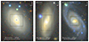 |
Fig. 1. Color-composite images of NGC 6860, Mrk 915, and MCG -01-24-012, generated with g − r − i − z filters from the archival Dark Energy Camera images. North is up and east is left, as in all other figures in the paper. The rectangles correspond to the FoV of the maps in Fig. 2. The central gray rectangle in the left image masks an artifact present in the i- and z-band images of NGC 6860. In Appendix A, we describe how these figures were generated. |
Table 1 shows some basic properties of the sample. The redshifts (z) correspond to the galaxies’ systemic velocities (vsys) and were obtained from kinematic 2D disk models fit to data in the regions dominated by rotation (Paper II). These redshifts were used to obtain the luminosity distances (DL) and the angular scales, by assuming a H0 = 70 km s−1, ΩM = 0.3, and ΩΛ = 0.7 cosmology.
Basic properties of the sample.
These Seyfert galaxies, with 0.014 < z < 0.025, have total AGN luminosities of 1043.6 ≲ LAGN ≲ 1044.8 erg s−1 and supermassive black hole masses of 107.1 ≲ MBH ≲ 108.4 M⊙, and their galaxy hosts have total stellar masses of 109.6 ≲ M* ≲ 1010.3 M⊙ (all references on Table 1). They are classified as Seyfert type 1.5, 1.9, or 2, according to the strength of the broad line region (BRL) component of the Hβ line (Osterbrock 1977).
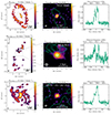 |
Fig. 2. Overview of the final reduced ALMA data, showing one object per row. Left: CO(2−1) moment M0, corresponding to the integrated flux. Center: ALMA millimeter continuum flux density near the CO spectral region, with M0 outline here with a bluish-green contour. Right: CO(2−1) spectral profile, integrated over the whole FoV (only spaxels not masked on the M0 map), showing the flux density vs. rest velocity (or observed frequency, in the top). The coordinates are relative to the galactic nucleus (black cross marks), assumed to be located at the ALMA millimeter continuum peak (see Table 1). The gray ellipses represent the ALMA beam resolution of the observation. |
3. Observations
3.1. ALMA
The three galaxies were observed with ALMA in Cycle 6 (ID: 2018.1.00211.S, PI: Ramakrishnan, V.). One of the spectral windows (SPWs) was centered on the CO(2−1) emission line. In addition, three other SPWs were centered on the nearby continuum. These were used to image the nuclear continuum and to subtract the underlying continuum from the line profiles. The total observing times on source for NGC 6860, Mrk 915, and MCG -01-24-012 were 33.9, 16.2, and 29.9 min, respectively. Table 2 shows other relevant information about the observations.
Information about ALMA observations, data reduction, and the total molecular mass.
We used the pipeline scripts provided by ALMA archive to reprocess the archival data using the CASA software (CASA Team 2022). Using this script, we performed typical reduction steps, including cross-calibration, flagging, and bandpass calibration. For the imaging, we used the tclean CASA’s task with the Briggs weighting scheme (Briggs 1995), which is controlled by the “robustness” parameter: a value of −2 is close to the uniform weighting, where the angular resolution is maximized at the expense of the sensitivity, with the opposite being true for a value of 2 (natural weighting).
For NGC 6860 and MCG01-24-012, we used a robustness parameter of 0 and 0.5, respectively. To improve the signal-to-noise ratio (S/N) of the Mrk 915, we used a robustness value of 2 to recover of the CO emission of Mrk 915 over a larger region inside the field of view (FoV). With the same goal, we also applied a Gaussian “uv taper” of 0.5″ to partially fill holes in the uv space. As was expected, this weighting scheme resulted in a poorer angular resolution in Mrk 915 compared to the other two objects, as is shown by the full width at half maximum (FWHM) of the beam in the table. The final spatial resolution is ∼0.5−0.8″ (∼150−400 pc), from the mean FWHMbeam. The angular samplings (spaxel sizes) of the cubes are 0.076″, 0.16″, and 0.087″ for NGC 6860, Mrk 915, and MCG -01-24-012, respectively.
To increase the S/N, the data cubes of the three objects were binned in pairs of two channels, with the resulting data cube having a channel width of Δv ∼ 10.2 km s−1. Table 2 also shows the corresponding σrms noise per channel at the center of the FoV. It corresponds to the standard deviation of the flux density in line-free regions prior to the primary beam correction (sensitivity over the FoV, a product from the data reduction). Throughout the paper, we used a 2D version σrms(x, y) = σrms/PB(x, y), where PB(x, y) is the primary beam map, which better replicates the increase in the noise toward the image edges.
An overall picture of the resulting reduced data is presented in Fig. 2. The maps of total CO(2−1) flux and the millimeter continuum flux density are shown in the left and middle columns, while the integrated CO(2−1) profile is shown in the right column. The continuum maps display an overall point-like spatial distribution, with only Mrk 915 showing a small elongation to the northwest.
The right ascensions (RAs) and declinations (DECs) in Table 1 correspond to the spatial coordinates of the peak of the ALMA 1.3 mm (230 GHz) continuum (middle column of Fig. 2, and marked as a cross in the other maps). We use this peak as the location of the AGN based on the correlation between 1 mm luminosity (L1 mm) with the 2−10 keV X-ray luminosity (L2 − 10 keV) and the black hole mass (MBH) in a plane (Ruffa et al. 2024). Comparing only with the X-ray continuum, there is a tighter correlation with L1 mm and L14 − 150 keV than L2 − 10 keV (Kawamuro et al. 2022). Nonetheless, the precise origin of the 1 mm emission is still uncertain and possibly not unique (Salvestrini et al. 2020; Kawamuro et al. 2023; Shablovinskaya et al. 2024), with some of the proposed explanations for the nuclear emission being small-scale jets and advection-dominated accretion flows (Ruffa et al. 2024). At the ALMA and HST spatial resolutions used here, the positions are expected to be coincident.
3.2. Archival data
For the ionized gas distribution, we used HST FR533N narrowband images (ID: 8598, Schmitt et al. 2003), which cover the [O III]λλ4959,5007 emission line region. To isolate the emission from the [O III] lines, F547M continuum images (from the same observation proposal) were subtracted from the narrowband [O III] ones. As is described in the Appendix B, the continuum image was multiplied by a constant factor (Kc) before being subtracted from the narrowband [O III] image. This factor was obtained interactively, by selecting the larger Kc value that does not introduce negative regions (“depressions”) in the subtracted image. However, we note that the F547M filter has a passband that partially covers the [O III] line profiles, which may induce over-subtraction of the line in some regions, particularly for NGC 6860 (see the Appendix B). The sky background of the resulting continuum-subtracted [O III] images was subtracted, after fitting a 2D plane in regions dominated by noise.
A visual inspection of the HST images indicated that they were spatially misaligned relative to the remaining images. Therefore, we modified their CRPIX/CRVAL header key values, such that the HST continuum peak matched the ALMA millimeter continuum peak. The CRPIX/CRVAL values for HST [O III] images were set equal to those of their respective F547M continuum images, which were aligned before. Comparing the resulting position of stars in the field in the HST and DECam images, we expect a maximum error in astrometry of∼0.1″.
All HST images were collected from the Mikulski Archive for Space Telescopes (MAST), selecting pipeline drizzled products. The reprocessing discussed above was applied to these images. The DECam images are from Data Release 10 (DR10) of the DESI Legacy Imaging Surveys.
For MCG -01-24-012 and Mrk 915, we also collected Very Large Array (VLA) archival 8.46 GHz (3.54 cm) radio images (Schmitt et al. 2001, proposal ID: AA226). The VLA images were downloaded from the NASA Extragalactic Database, without further modifications.
4. Analysis
4.1. Structure maps
To highlight morphological stellar features in the host galaxies, we constructed structure maps using images of the sources, as is shown in Fig. 3. With such a technique, structures with scales on the order of the point spread function (∼500 pc) are enhanced (Pogge & Martini 2002).
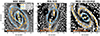 |
Fig. 3. Structure maps, with dashed lines and curves highlighting spiral arms (in orange), stellar rings (sky-blue), and bars (yellow). The lines were drawn by visual inspection of the top structure maps, obtained for the archival DECam i-band images, where structures with spatial scales of ∼500 pc are enhanced. |
Following Simões Lopes et al. (2007), these structure maps (S) were obtained using (Pogge & Martini 2002)
![Mathematical equation: $$ \begin{aligned} S = \left[\frac{I}{I\otimes P}\right] \otimes P^t, \end{aligned} $$](/articles/aa/full_html/2025/09/aa52993-24/aa52993-24-eq1.gif) (1)
(1)
where I is the original image, and P is the point spread function. To obtain the PSF, we modeled the flux distributions of field stars with Moffat profiles (e.g., Trujillo et al. 2001). The fitting and convolution procedures were performed using ASTROPY.MODELING and ASTROPY.CONVOLVE.
Dashed lines in Fig. 3 mark the location of spiral arms, rings, and bars, all identified by visual inspection. We obtained the structure maps using DECam i-band images (covering 710−860 nm) because we wanted to highlight stellar bars, and the light from such structures is dominated by the contribution from old stars, whose emission peak is seen at longer wavelengths.
4.2. Molecular gas mass
The total velocity-integrated flux (SνΔvCO(2 − 1)) and the derived CO(2−1) luminosity (L′CO(2 − 1)) and molecular mass (Mmol) are presented in Table 2. The CO flux – in each spaxel – was derived from the Gaussian profiles fit to the CO profile, with a maximum of two components being needed to reproduce each profile (Paper II). The corresponding uncertainties were obtained following Lenz & Ayres (1992) and are propagated when integrated over a region and/or including more than one component. The corresponding luminosities (L′CO(2 − 1)), in units of K km s−1 pc−2, were obtained using Equation (1) from Solomon et al. (1997). We converted the resulting values to CO(1−0) luminosities by using the ratio of r21 = L′CO(2 − 1)/L′CO(1 − 0) = 0.8 − 1.2, observed in nearby galaxies (Braine & Combes 1992).
The molecular mass can then be calculated using the conversion factor αCO = Mmol/L′CO(1 − 0). To cover different cloud physical conditions, we assumed a large range of values: αCO = MH2/L′CO(1 − 0) = 0.8 − 4.3 M⊙ [K km s−1 pc−2]−1. The upper limit value in the above αCO corresponds to the average in the Milky Way inner disk, while the lower limit is the average in ultraluminous infrared galaxies (Bolatto et al. 2013).
In addition to the large uncertainties in the CO-to-H2 conversion, we note that the total CO(2−1) luminosities used in the calculation may be systematically underestimated. This happens because interferometric observations filter out large-scale emission, causing low-surface brightness CO(2−1) emission to be missed. This issue is sometimes referred to as the “missing flux problem”. As a consequence, our total CO fluxes and Mmol, tot measurements can be considered lower limit values.
To illustrate this, we can compare our total flux measurements with values obtained using single-dish telescopes. For NGC 6860, Strong et al. (2004) obtained CO(2−1) observations with the Swedish–ESO Submillimetre Telescope (SEST, with FWHMbeam of 22″), resulting in L′CO(2 − 1) = 23 × 107 K km s−1 pc−2 (value corrected to consider the same cosmology parameters assume here). This value is a factor of ∼2 larger than our measurement of L′CO(2 − 1) ∼ 11.8 × 10⁷ K km s−1 pc−2. Similarly, Koss et al. (2021) presented observations of our objects from the Atacama Pathfinder Experiment telescope (APEX, FWHMbeam of 27″), with CO(2−1) luminosity values that are larger than our measurements by a factor of ∼3 for NGC 6860 and MCG -01-24-012, and ∼6 for Mrk 915. In addition, CO emission from regions beyond the FoV of our ALMA observations may also contribute to the single dish measurements. For comparison, the FWHMbeam of these SEST and APEX observations are, respectively, ∼1.3 and 1.7 times larger than our observations’ FoV (∼17″ radius, at one quarter of the sensitivity of the FoV center).
5. Results: CO versus [O III] relation
In the central kiloparsec, the flux distributions of the [O III] and the CO(2−1) are spatially anticorrelated in our sample. This is shown by the contours comparing the CO(2−1) and [O III] flux distributions in Fig. 4. Also displayed is the 3.6 cm radio emission available for Mrk 915 and MCG -01-24-012.
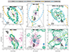 |
Fig. 4. Contours showing the flux distribution from the CO(2−1) cold molecular gas (M0, in bluish-green), [O III] ionized gas (reddish-purple), and the 3.6 cm radio (blue), with a zoom-in of the nuclear 3″ × 3″ region (bottom panels). The dashed yellow, orange, and sky-blue lines correspond to stellar bar, spiral arm, and stellar ring structures, respectively (identified in Fig. 4). Colored ellipses represent the beam resolutions of each contour image, using the same color as the tracer. Contours are evenly spaced logarithmically. There are: 10 CO(2−1) contour levels in the ranges (0.508, 47.8), (0.620, 28.0), and (0.359, 93.5) Jy km s−1, for NGC 6860, Mrk 915, and MCG -01-24-012, respectively; 10 [O III] levels in the ranges (10−18.3, 10−16.4), (10−18.2, 10−15.7), and (10−18.3, 10−16.2) erg s−1 cm−2 Å, in the same order; and 4 radio levels in the ranges (10.2, 1202) and (10.35, 713) mJy, for Mrk 915 and MCG -01-24-012. |
In NGC 6860, the CO(2−1) emission is observed along the stellar ring and the bar (inside a r ∼ 4 kpc projected radius from the nucleus), corresponding to a total cold molecular gas mass of Mmol, tot ∼ 8 − 60 × 107 M⊙. We notice that, close to the nucleus (r ∼ 500 pc), the CO emission presents an hourglass shape: the projected emission shows a narrowing width as it approaches the nucleus, decreasing from ∼400−500 pc to ∼250 pc in width (lower left map of Fig. 4). Interestingly, the [O III] bipolar emission – extending in the east-west direction – seems to fill the region where the CO flux distribution is narrower, with the [O III] contours forming a “bowl shape” at the base of the emission.
In Mrk 915, the cold molecular gas is observed along the two central spiral arms, totalizing Mmol, tot ∼ 2 − 20 × 107 M⊙. Unlike the other two Seyferts, the [O III] ionized gas in Mrk 915 does not present a bipolar morphology, in the sense of the [O III] being elongated in opposite and aligned directions (lower middle panel in Fig. 4). Instead, it is spatially elongated in two directions: north (position angle (PA) ∼ 5°) and southwest of the nucleus (PA ∼ 210−235°). Also extended to the southwest of the nucleus, there is a weak 3.6 cm radio source that could indicate the projected direction of a young radio-jet axis, although further observations are needed to better resolve and confirm the jet. Additionally, to verify a young-source origin for the emission, it is necessary to calculate the radio spectral index, which depends on the availability of multiband radio observations (e.g., Kukreti et al. 2023). Nonetheless, except in the nucleus, we still observe a spatial anticorrelation between CO and [O III] flux distributions.
In MCG -01-24-012, most of Mmol, tot ∼ 9 − 70 × 107 M⊙ cold molecular mass, traced by CO emission, is detected in the stellar ring and the area within it. Within this region, the observed CO flux distribution is not only concentrated near the bar (as in NGC 6860), but more spread out. Within the inner 2.5″ ∼1 kpc radius, the strongest CO emission is distributed in the north-south direction, with a small twist to the northeast at larger radii (right panel in Fig. 4). This distribution is approximately perpendicular to that of the [O III] bipolar emission, which has PA ∼ 75° (Schmitt et al. 2003). We also note that the 3.6 cm radio emission has a small elongation to the west (PA ∼ 89°, Schmitt et al. 2001), approximately aligned with the [O III] ionization axis.
6. Discussions
A strong spatial anticorrelation between the cold molecular and ionized gas and/or the radio jet has already been observed in other active galaxies (e.g., García-Bernete et al. 2021; Audibert et al. 2023; Alonso-Herrero et al. 2018). We found the same trend for the three sources studied here: NGC 6860, Mrk 915, and MCG -01-24-012.
Of the remaining 10 objects in our original sample (there were 13 sources in total), 6 have been the subject of individual studies comparing the CO versus jets and/or ionized gas emissions, and 5 of them – all showing extended bipolar ionized cones/jets – follow the above anticorrelation trend: NGC 3281 (Dall’Agnol de Oliveira et al. 2023), NGC 3393 (Finlez et al. 2018), ESO 428-G14 (Feruglio et al. 2020), NGC 2110 (Rosario et al. 2019), and NGC 5728 (Shimizu et al. 2019). In NGC 1566, there is a CO deficit in the nucleus (Slater et al. 2019), where ionized gas emission is unresolved under ∼50 pc, (da Silva et al. 2017). For the remaining 4 objects, we performed a visual inspection using CO and ionized gas images from different studies. We identified a CO gap (Ramakrishnan et al. 2019; Salvestrini et al. 2020) associated with the bipolar ionization cone in NGC 1386 (Rodríguez-Ardila et al. 2017, ∼100 pc to the north of the nucleus), NGC 7213 (Schnorr-Müller et al. 2014, ∼300 pc to the southwest), and NGC 3081 (Schnorr-Müller et al. 2016, southwest to northeast direction, under a ∼600 pc radius). In NGC 1667, a local CO deficit is visible (Ramakrishnan et al. 2019) where the ionized gas emission is slightly elongated (∼400 pc to the east) and where it is more disturbed (Schnorr-Müller et al. 2017, southeast to northwest direction). Overall, we found some degree of spatial anticorrelation between CO and ionized gas and/or jets in 12 out of 13 objects from the original sample.
To understand the cause behind this, we can first focus on the three sources presented here. A possible scenario is that part of the molecular gas is being dissociated by AGN radiation, winds, and/or jets. This assumes that the [O III] extended emission traces the AGN ionization axis, which is corroborated by the bipolar [O III] flux distribution in NGC 6860 and MCG -01-24-012. Also, Mrk 915 and MCG -01-24-012 show weak off-nuclear 3.6 cm radio emission, which extends in one of the directions in which the [O III] emission is elongated.
In favor of this, in NGC 2110, Kawamuro et al. (2020) also observed an anticorrelation between the flux distribution of the CO and the Fe-Kα 6.4 keV fluorescent line, which needs ionization from hard X-ray photons to be produced. This reinforces the scenario that the CO or/and H2 may be depleted due to the high-energy photons from the AGN. A similar conclusion may be drawn for NGC 5728, where the X-ray emission containing highly ionized lines is observed in the region devoid of CO gas (Trindade Falcao et al. 2024). However, the presence of cold scattering material may indicate that part of the molecular gas could still be present along the ionization axis (see below).
We emphasize that an observed spatial anticorrelation between CO emission and ionized gas is not definitive evidence that molecular gas is being destroyed. For example, the AGN radiation could be ionizing the gas located in (or the ionized outflow could be expanding to) regions already devoid of cold molecules. Besides that, even if we follow the hypothesis that CO emission gaps are a consequence of CO molecules being partially destroyed, H2 molecules might still survive in these depleted regions.
For example, in NGC 2110, emission from the hot H2 1−0 S(1) line1 is detected in a CO(2−1) lacuna (Rosario et al. 2019). A similar scenario is observed in the Seyfert galaxies NGC 5643 (Alonso-Herrero et al. 2018; Davies et al. 2014) and ESO 428-G14 (Feruglio et al. 2020), both on CO(2−1) and H2 1−0 S(1) transitions. Another example is NGC 5728, with emission from the warm H2 0−0 S(3) line2 being observed throughout the ionization cone, where there is a CO deficit (Davies et al. 2024). Other warm H2 0−0 S(1), S(5) (Davies et al. 2024) and hot H2 1−0 S(1) lines (Shimizu et al. 2019) are also detected in the gap of the CO in NCG 5728. In MCG -05-23-16, warm H2 gas (from multiple transitions) is detected in the CO(2−1) cavities, in a region where H2 displays higher velocity dispersion, likely driven by recent star formation in this case Esparza-Arredondo et al. (2025).
After comparing mass surface densities on 50 and 200 pc scales in Seyfert galaxies, García-Burillo et al. (2024) found a decrease in the concentration in both the cold and hot molecular gas phases for X-ray luminosities above L2 − 10 KeV ∼ 1041.5 erg s−1. They interpret that the AGN radiation-driven winds or jets have pushed out the H2 gas, since the most extreme nuclear-scale cold molecular gas deficits are observed in galaxies with the strongest CO outflows. This is in agreement with our results, since the X-ray luminosities of our objects are a factor of ∼10 above this threshold (Duras et al. 2020). Nonetheless, their deficit in the cold molecular gas is not fully compensated for (filled) by the hot molecular phase emission.
We note that in high-spatial-resolution (50−100 pc scale) observations of star-forming regions, the CO versus Hα distribution shows that the cold molecular gas is also anticorrelated in areas with recent star formation (Leroy et al. 2021; Kreckel et al. 2018), although there is some overlap in denser areas, as in spiral arms (Larson et al. 2023). The ionizing radiation from the newly born stars is likely depleting the nearby CO molecular clouds inside H II regions (traced by Hα). This is similar to what is observed in our sources, but for a weaker ionization field.
As a final remark, we point out that the maximum recoverable scale of emission in our ALMA observations is ∼6″ (∼2−3 kpc). Emission from larger scales will therefore not be detected in our data. This could be why we measure a total CO flux ∼2−6 times lower than in the single-dish observations (see Section 4.2), which do not suffer from the missing flux problem. However, this is unlikely to be the reason behind the observed CO gaps, since they are identified on smaller scales (≲1 kpc, see Fig. 4). Any CO emission present at these scales would have been detected with the sensitivity of the ALMA data. We therefore propose that these CO gaps show a real inhomogeneity in the CO distribution.
7. Conclusions
We have compared the CO cold molecular gas distributions – traced by CO(2−1) ALMA observations – with the [O III] ionized gas distributions – from HST images – of three nearby Seyfert galaxies and compared them with the results for the original sample of 13 active galaxies. The main conclusions are:
-
There is a spatial anticorrelation between the cold molecular gas and ionized gas distributions in the three galaxies studied, observed within the inner kiloparsec. Evidence of the same trend is presented in other studies in the literature, including 12 out of 13 nearby AGN sources from our original sample.
-
The anticorrelation can be attributed – in part – to a depletion of the cold molecular gas due to the AGN radiation, winds, and/or jets. Warmer phases of the molecular gas (e.g., infrared H2 lines) might fill part of the CO gap region.
Assuming that the observed CO deficit is due to an interaction between the AGN released energy and the ISM, one can argue that this is a type of AGN negative feedback not accounted for when measuring the impact using quantities such as the mass outflow rate. In our Paper II, we present measurements of this impact obtained from the analysis of the CO(2−1) kinematics. However, to fully discriminate how much of the molecular gas is completely depleted, measurements of the distribution and total mass of the molecular gas at different temperatures are needed.
Near-infrared rovibrational transition, Tgas ∼103 K.
Mid-infrared pure rotational transition, Tgas ∼ 102 − 103 K.
Acknowledgments
This study was financed in part by the Coordenação de Aperfeiçoamento de Pessoal de Nível Superior (CAPES-Brasil, 88887.478902/2020-00, 88887.985730/2024-00). RAR acknowledges the support from Conselho Nacional de Desenvolvimento Científico e Tecnológico (CNPq; Proj. 303450/2022-3, 403398/2023-1, & 441722/2023-7), Fundação de Amparo à pesquisa do Estado do Rio Grande do Sul (FAPERGS; Proj. 21/2551-0002018-0), and CAPES (Proj. 88887.894973/2023-00). This paper makes use of the following ALMA data: ADS/JAO.ALMA#2018.1.00211.S, ADS/JAO.ALMA#2015.1.00086.S, ADS/JAO.ALMA#2012.1.00474.S. ALMA is a partnership of ESO (representing its member states), NSF (USA) and NINS (Japan), together with NRC (Canada), MOST and ASIAA (Taiwan), and KASI (Republic of Korea), in cooperation with the Republic of Chile. The Joint ALMA Observatory is operated by ESO, AUI/NRAO and NAOJ. The Legacy Surveys consist of three individual and complementary projects: the Dark Energy Camera Legacy Survey (DECaLS; Proposal ID #2014B-0404; PIs: David Schlegel and Arjun Dey), the Beijing-Arizona Sky Survey (BASS; NOAO Prop. ID #2015A-0801; PIs: Zhou Xu and Xiaohui Fan), and the Mayall z-band Legacy Survey (MzLS; Prop. ID #2016A-0453; PI: Arjun Dey). DECaLS, BASS and MzLS together include data obtained, respectively, at the Blanco telescope, Cerro Tololo Inter-American Observatory, NSF’s NOIRLab; the Bok telescope, Steward Observatory, University of Arizona; and the Mayall telescope, Kitt Peak National Observatory, NOIRLab. Pipeline processing and analyses of the data were supported by NOIRLab and the Lawrence Berkeley National Laboratory (LBNL). The Legacy Surveys project is honored to be permitted to conduct astronomical research on Iolkam Du’ag (Kitt Peak), a mountain with particular significance to the Tohono O’odham Nation. This research has made use of the NASA/IPAC Extragalactic Database, which is funded by the National Aeronautics and Space Administration and operated by the California Institute of Technology. This work used the color scheme from Wong (2011) in some of the plots to minimize confusion for colorblind viewers.
References
- Alonso-Herrero, A., Pereira-Santaella, M., García-Burillo, S., et al. 2018, ApJ, 859, 144 [Google Scholar]
- Audibert, A., Ramos Almeida, C., García-Burillo, S., et al. 2023, A&A, 671, L12 [NASA ADS] [CrossRef] [EDP Sciences] [Google Scholar]
- Ballo, L., Severgnini, P., Della Ceca, R., et al. 2017, MNRAS, 470, 3924 [Google Scholar]
- Bennert, N., Jungwiert, B., Komossa, S., Haas, M., & Chini, R. 2006, A&A, 459, 55 [NASA ADS] [CrossRef] [EDP Sciences] [Google Scholar]
- Bolatto, A. D., Wolfire, M., & Leroy, A. K. 2013, ARA&A, 51, 207 [CrossRef] [Google Scholar]
- Braine, J., & Combes, F. 1992, A&A, 264, 433 [NASA ADS] [Google Scholar]
- Briggs, D. S. 1995, Ph.D. Thesis, New Mexico Institute of Mining and Technology [Google Scholar]
- CASA Team (Bean, B., et al.) 2022, PASP, 134, 114501 [NASA ADS] [CrossRef] [Google Scholar]
- Cicone, C., Brusa, M., Ramos Almeida, C., et al. 2018, Nat. Astron., 2, 176 [Google Scholar]
- da Silva, P., Steiner, J. E., & Menezes, R. B. 2017, MNRAS, 470, 3850 [Google Scholar]
- Dall’Agnol de Oliveira, B., Storchi-Bergmann, T., Kraemer, S. B., et al. 2021, MNRAS, 504, 3890 [CrossRef] [Google Scholar]
- Dall’Agnol de Oliveira, B., Storchi-Bergmann, T., Morganti, R., Riffel, R. A., & Ramakrishnan, V. 2023, MNRAS, 522, 3753 [CrossRef] [Google Scholar]
- Dall’Agnol de Oliveira, B., Storchi-Bergmann, T., Morganti, R., et al. 2025, A&A, submitted (Paper II) [Google Scholar]
- Davies, R. I., Maciejewski, W., Hicks, E. K. S., et al. 2014, ApJ, 792, 101 [Google Scholar]
- Davies, R., Baron, D., Shimizu, T., et al. 2020, MNRAS, 498, 4150 [Google Scholar]
- Davies, R., Shimizu, T., Pereira-Santaella, M., et al. 2024, A&A, 689, A263 [NASA ADS] [CrossRef] [EDP Sciences] [Google Scholar]
- Duras, F., Bongiorno, A., Ricci, F., et al. 2020, A&A, 636, A73 [NASA ADS] [CrossRef] [EDP Sciences] [Google Scholar]
- Esparza-Arredondo, D., Ramos Almeida, C., Audibert, A., et al. 2025, A&A, 693, A174 [NASA ADS] [CrossRef] [EDP Sciences] [Google Scholar]
- Feruglio, C., Fabbiano, G., Bischetti, M., et al. 2020, ApJ, 890, 29 [Google Scholar]
- Finlez, C., Nagar, N. M., Storchi-Bergmann, T., et al. 2018, MNRAS, 479, 3892 [Google Scholar]
- Fischer, T. C., Crenshaw, D. M., Kraemer, S. B., & Schmitt, H. R. 2013, ApJS, 209, 1 [Google Scholar]
- Fischer, T. C., Kraemer, S. B., Schmitt, H. R., et al. 2018, ApJ, 856, 102 [Google Scholar]
- García-Bernete, I., Alonso-Herrero, A., García-Burillo, S., et al. 2021, A&A, 645, A21 [EDP Sciences] [Google Scholar]
- García-Burillo, S., Hicks, E. K. S., Alonso-Herrero, A., et al. 2024, A&A, 689, A347 [NASA ADS] [CrossRef] [EDP Sciences] [Google Scholar]
- Goodrich, R. W. 1995, ApJ, 440, 141 [CrossRef] [Google Scholar]
- Heckman, T. M., & Best, P. N. 2014, ARA&A, 52, 589 [Google Scholar]
- Hernández-Yévenes, J., Nagar, N., Arratia, V., & Jarrett, T. H. 2024, MNRAS, 531, 4503 [Google Scholar]
- Karouzos, M., Woo, J.-H., & Bae, H.-J. 2016, ApJ, 819, 148 [NASA ADS] [CrossRef] [Google Scholar]
- Kawamuro, T., Izumi, T., Onishi, K., et al. 2020, ApJ, 895, 135 [NASA ADS] [CrossRef] [Google Scholar]
- Kawamuro, T., Ricci, C., Imanishi, M., et al. 2022, ApJ, 938, 87 [NASA ADS] [CrossRef] [Google Scholar]
- Kawamuro, T., Ricci, C., Mushotzky, R. F., et al. 2023, ApJS, 269, 24 [NASA ADS] [CrossRef] [Google Scholar]
- Koss, M. J., Strittmatter, B., Lamperti, I., et al. 2021, ApJS, 252, 29 [CrossRef] [Google Scholar]
- Kreckel, K., Faesi, C., Kruijssen, J. M. D., et al. 2018, ApJ, 863, L21 [NASA ADS] [CrossRef] [Google Scholar]
- Kukreti, P., Morganti, R., Tadhunter, C., & Santoro, F. 2023, A&A, 674, A198 [NASA ADS] [CrossRef] [EDP Sciences] [Google Scholar]
- La Franca, F., Onori, F., Ricci, F., et al. 2015, MNRAS, 449, 1526 [Google Scholar]
- Larson, K. L., Lee, J. C., Thilker, D. A., et al. 2023, MNRAS, 523, 6061 [NASA ADS] [CrossRef] [Google Scholar]
- Lenz, D. D., & Ayres, T. R. 1992, PASP, 104, 1104 [NASA ADS] [CrossRef] [Google Scholar]
- Leroy, A. K., Schinnerer, E., Hughes, A., et al. 2021, ApJS, 257, 43 [NASA ADS] [CrossRef] [Google Scholar]
- Lipari, S., Tsvetanov, Z., & Macchetto, F. 1993, ApJ, 405, 186 [Google Scholar]
- Liu, G., Zakamska, N. L., Greene, J. E., Nesvadba, N. P. H., & Liu, X. 2013, MNRAS, 436, 2576 [NASA ADS] [CrossRef] [Google Scholar]
- Lupton, R., Blanton, M. R., Fekete, G., et al. 2004, PASP, 116, 133 [NASA ADS] [CrossRef] [Google Scholar]
- Middei, R., Matzeu, G. A., Bianchi, S., et al. 2021, A&A, 647, A102 [NASA ADS] [CrossRef] [EDP Sciences] [Google Scholar]
- Onori, F., La Franca, F., Ricci, F., et al. 2017, MNRAS, 464, 1783 [NASA ADS] [CrossRef] [Google Scholar]
- Osterbrock, D. E. 1977, ApJ, 215, 733 [Google Scholar]
- Pogge, R. W., & Martini, P. 2002, ApJ, 569, 624 [CrossRef] [Google Scholar]
- Ramakrishnan, V., Nagar, N. M., Finlez, C., et al. 2019, MNRAS, 487, 444 [Google Scholar]
- Ramos Almeida, C., Bischetti, M., García-Burillo, S., et al. 2022, A&A, 658, A155 [NASA ADS] [CrossRef] [EDP Sciences] [Google Scholar]
- Revalski, M., Meena, B., Martinez, F., et al. 2021, ApJ, 910, 139 [NASA ADS] [CrossRef] [Google Scholar]
- Revalski, M., Crenshaw, D. M., Rafelski, M., et al. 2022, ApJ, 930, 14 [NASA ADS] [CrossRef] [Google Scholar]
- Riffel, R. A., Dors, O. L., Armah, M., et al. 2021, MNRAS, 501, L54 [Google Scholar]
- Riffel, R. A., Riffel, R., Storchi-Bergmann, T., et al. 2024, MNRAS, 528, 1476 [Google Scholar]
- Rodríguez-Ardila, A., Prieto, M. A., Mazzalay, X., et al. 2017, MNRAS, 470, 2845 [Google Scholar]
- Rosario, D. J., Togi, A., Burtscher, L., et al. 2019, ApJ, 875, L8 [NASA ADS] [CrossRef] [Google Scholar]
- Ruffa, I., Davis, T. A., Elford, J. S., et al. 2024, MNRAS, 528, L76 [Google Scholar]
- Saintonge, A., & Catinella, B. 2022, ARA&A, 60, 319 [NASA ADS] [CrossRef] [Google Scholar]
- Salvestrini, F., Gruppioni, C., Pozzi, F., et al. 2020, A&A, 641, A151 [NASA ADS] [CrossRef] [EDP Sciences] [Google Scholar]
- Schinnerer, E., & Leroy, A. K. 2024, ARA&A, 62, 369 [NASA ADS] [CrossRef] [Google Scholar]
- Schmitt, H. R., Ulvestad, J. S., Antonucci, R. R. J., & Kinney, A. L. 2001, ApJS, 132, 199 [NASA ADS] [CrossRef] [Google Scholar]
- Schmitt, H. R., Donley, J. L., Antonucci, R. R. J., Hutchings, J. B., & Kinney, A. L. 2003, ApJS, 148, 327 [NASA ADS] [CrossRef] [Google Scholar]
- Schnorr-Müller, A., Storchi-Bergmann, T., Nagar, N. M., & Ferrari, F. 2014, MNRAS, 438, 3322 [Google Scholar]
- Schnorr-Müller, A., Storchi-Bergmann, T., Robinson, A., Lena, D., & Nagar, N. M. 2016, MNRAS, 457, 972 [Google Scholar]
- Schnorr-Müller, A., Storchi-Bergmann, T., Ferrari, F., & Nagar, N. M. 2017, MNRAS, 466, 4370 [NASA ADS] [Google Scholar]
- Shablovinskaya, E., Ricci, C., Chang, C. S., et al. 2024, A&A, 690, A232 [NASA ADS] [CrossRef] [EDP Sciences] [Google Scholar]
- Shimizu, T. T., Davies, R. I., Lutz, D., et al. 2019, MNRAS, 490, 5860 [Google Scholar]
- Simões Lopes, R. D., Storchi-Bergmann, T., de Fátima Saraiva, M., & Martini, P. 2007, ApJ, 655, 718 [Google Scholar]
- Slater, R., Nagar, N. M., Schnorr-Müller, A., et al. 2019, A&A, 621, A83 [NASA ADS] [CrossRef] [EDP Sciences] [Google Scholar]
- Solomon, P. M., Downes, D., Radford, S. J. E., & Barrett, J. W. 1997, ApJ, 478, 144 [NASA ADS] [CrossRef] [Google Scholar]
- Storchi-Bergmann, T., Wilson, A. S., & Baldwin, J. A. 1992, ApJ, 396, 45 [Google Scholar]
- Storchi-Bergmann, T., Dall’Agnol de Oliveira, B., Longo Micchi, L. F., et al. 2018, ApJ, 868, 14 [Google Scholar]
- Strong, M., Pedlar, A., Aalto, S., et al. 2004, MNRAS, 353, 1151 [Google Scholar]
- Sun, A.-L., Greene, J. E., & Zakamska, N. L. 2017, ApJ, 835, 222 [Google Scholar]
- Trindade Falcao, A., Fabbiano, G., Elvis, M., et al. 2024, ApJ, 963, 6 [Google Scholar]
- Trippe, M. L., Crenshaw, D. M., Deo, R. P., et al. 2010, ApJ, 725, 1749 [NASA ADS] [CrossRef] [Google Scholar]
- Trujillo, I., Aguerri, J. A. L., Cepa, J., & Gutiérrez, C. M. 2001, MNRAS, 328, 977 [NASA ADS] [CrossRef] [Google Scholar]
- Véron-Cetty, M. P., & Véron, P. 2006, A&A, 455, 773 [Google Scholar]
- Wilson, A. S., Braatz, J. A., Heckman, T. M., Krolik, J. H., & Miley, G. K. 1993, ApJ, 419, L61 [NASA ADS] [CrossRef] [Google Scholar]
- Winter, L. M., Mushotzky, R. F., Reynolds, C. S., & Tueller, J. 2009, ApJ, 690, 1322 [NASA ADS] [CrossRef] [Google Scholar]
- Wong, B. 2011, Nat. Meth., 8, 441 [Google Scholar]
- Wylezalek, D., & Zakamska, N. L. 2016, MNRAS, 461, 3724 [NASA ADS] [CrossRef] [Google Scholar]
Appendix A: RGB color-composite image
To emphasize stellar structures in the central regions of our objects, we generated the griz color-composite images using archival DECam images from DESI. We applied the GET_RGB function from the DESI Imaging Legacy Surveys viewer pipeline3. This function implements an algorithm based on Lupton et al. (2004), with the RGB components obtained from a scaling of the griz-band filters images: R = (3 ⋅ i + 2.2 ⋅ z), G = (3.4 ⋅ r) and B = (6 ⋅ g). To highlight features in the central regions, we ran the original code, changing the default asinh softening value (Q) from 20 to 50 (see the result in Fig. 1).
Appendix B: [O III] continuum subtraction in NGC 6860
The [O III] maps were obtained by subtracting the FR533N narrowband image ([O III] + continuum) from the medium-band F547M image (nearby continuum) multiplied by a Kc factor: [O III] = (FR533N) − Kc ⋅ (F547M). This factor is interactively chosen, by maximizing the removal of the continuum contribution without introducing extended regions with negative values (continuum oversubtraction). However, this method introduces negative values in the central pixels of NGC 6860 (upper right image of Fig. B.1). The problem happens because a small part of the F547M band covers the [O III]λ5007 lines when its flux is stronger or its profile width is wider, resulting in an overestimation of the continuum at the nucleus.
For the final [O III] image, the optical continuum was better subtracted using Kc = 1.14. To remove the resulting negative values in the center, we interpolated the flux in this region (lower right image of Fig. B.1). The resulting [O III] contours are similar to the original data published in Schmitt et al. (2003).
The left image of Fig. B.1 shows the result of choosing a Kc factor that avoids negative flux values at the nucleus. The [O III] would be more extended following the continuum, up to the stellar ring. The [O III] observations from Lipari et al. (1993) show that there is [O III] emission in the stellar ring, but their total exposure time is ∼ 2 times longer. Nonetheless, the nuclear [O III] morphology is consistent in the three cases of Fig. B.1).
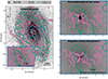 |
Fig. B.1. The effect on the [O III] flux distribution (reddish-purple contours) when the HST F547M optical continuum image (in grayscale) is multiplied by different factors before the subtraction from the FR533N image (narrow band filter covering [O III]). In the left, the continuum F547M was undersubtracted from [O III] – using a lower multiplicative factor – to avoid negative values are the center, with the inset showing a zoom-in in the central region. Notice that the smoothed [O III] contours follow the extended continuum distribution in this case. On the right, the continuum was subtracted using a larger factor that resulted in negative values at the center (upper map). For the final image, the [O III] image was interpolated to eliminate the negative values (lower map). To show that the spatial anticorrelation between CO and [O III] is visible in both maps, we added a single blueish-green contour, delineating the CO(2-1) flux distribution. In all zoom-in images, the F547M grayscale range is different maps to highlight the peak in the F547M image. |
All Tables
Information about ALMA observations, data reduction, and the total molecular mass.
All Figures
|
Fig. 1. Color-composite images of NGC 6860, Mrk 915, and MCG -01-24-012, generated with g − r − i − z filters from the archival Dark Energy Camera images. North is up and east is left, as in all other figures in the paper. The rectangles correspond to the FoV of the maps in Fig. 2. The central gray rectangle in the left image masks an artifact present in the i- and z-band images of NGC 6860. In Appendix A, we describe how these figures were generated. |
| In the text | |
|
Fig. 2. Overview of the final reduced ALMA data, showing one object per row. Left: CO(2−1) moment M0, corresponding to the integrated flux. Center: ALMA millimeter continuum flux density near the CO spectral region, with M0 outline here with a bluish-green contour. Right: CO(2−1) spectral profile, integrated over the whole FoV (only spaxels not masked on the M0 map), showing the flux density vs. rest velocity (or observed frequency, in the top). The coordinates are relative to the galactic nucleus (black cross marks), assumed to be located at the ALMA millimeter continuum peak (see Table 1). The gray ellipses represent the ALMA beam resolution of the observation. |
| In the text | |
|
Fig. 3. Structure maps, with dashed lines and curves highlighting spiral arms (in orange), stellar rings (sky-blue), and bars (yellow). The lines were drawn by visual inspection of the top structure maps, obtained for the archival DECam i-band images, where structures with spatial scales of ∼500 pc are enhanced. |
| In the text | |
|
Fig. 4. Contours showing the flux distribution from the CO(2−1) cold molecular gas (M0, in bluish-green), [O III] ionized gas (reddish-purple), and the 3.6 cm radio (blue), with a zoom-in of the nuclear 3″ × 3″ region (bottom panels). The dashed yellow, orange, and sky-blue lines correspond to stellar bar, spiral arm, and stellar ring structures, respectively (identified in Fig. 4). Colored ellipses represent the beam resolutions of each contour image, using the same color as the tracer. Contours are evenly spaced logarithmically. There are: 10 CO(2−1) contour levels in the ranges (0.508, 47.8), (0.620, 28.0), and (0.359, 93.5) Jy km s−1, for NGC 6860, Mrk 915, and MCG -01-24-012, respectively; 10 [O III] levels in the ranges (10−18.3, 10−16.4), (10−18.2, 10−15.7), and (10−18.3, 10−16.2) erg s−1 cm−2 Å, in the same order; and 4 radio levels in the ranges (10.2, 1202) and (10.35, 713) mJy, for Mrk 915 and MCG -01-24-012. |
| In the text | |
|
Fig. B.1. The effect on the [O III] flux distribution (reddish-purple contours) when the HST F547M optical continuum image (in grayscale) is multiplied by different factors before the subtraction from the FR533N image (narrow band filter covering [O III]). In the left, the continuum F547M was undersubtracted from [O III] – using a lower multiplicative factor – to avoid negative values are the center, with the inset showing a zoom-in in the central region. Notice that the smoothed [O III] contours follow the extended continuum distribution in this case. On the right, the continuum was subtracted using a larger factor that resulted in negative values at the center (upper map). For the final image, the [O III] image was interpolated to eliminate the negative values (lower map). To show that the spatial anticorrelation between CO and [O III] is visible in both maps, we added a single blueish-green contour, delineating the CO(2-1) flux distribution. In all zoom-in images, the F547M grayscale range is different maps to highlight the peak in the F547M image. |
| In the text | |
Current usage metrics show cumulative count of Article Views (full-text article views including HTML views, PDF and ePub downloads, according to the available data) and Abstracts Views on Vision4Press platform.
Data correspond to usage on the plateform after 2015. The current usage metrics is available 48-96 hours after online publication and is updated daily on week days.
Initial download of the metrics may take a while.