| Issue |
A&A
Volume 701, September 2025
|
|
|---|---|---|
| Article Number | A282 | |
| Number of page(s) | 20 | |
| Section | Numerical methods and codes | |
| DOI | https://doi.org/10.1051/0004-6361/202553654 | |
| Published online | 25 September 2025 | |
Owl-z: Bayesian tool for selecting z ≳ 7 quasars
1
Aix Marseille Univ, CNRS, CNES, LAM, Marseille, France
2
Aix Marseille Univ, CNRS, I2M, Marseille, France
3
Aix Marseille Univ, CNRS, LIS, Marseille, France
4
Canada-France-Hawai’i Telescope, Waimea, Hawai’i, USA
5
Université Paris-Saclay, Université Paris Cité, CEA, CNRS, AIM, 91191 Gif-sur-Yvette, France
6
Leiden Observatory, Leiden University, PO Box 9513, 2300 RA Leiden, The Netherlands
★ Corresponding author: This email address is being protected from spambots. You need JavaScript enabled to view it.
Received:
1
January
2025
Accepted:
2
July
2025
Abstract
This paper presents Owl-z, a Bayesian code aimed at identifying z ≥ 7 quasars in wide-field optical and near-infrared surveys. By construction, the code can also be used to select objects that contaminate the high-z quasar population, such as brown dwarfs and early-type galaxies at intermediate redshifts. The code can be adapted for the selection of high-z galaxies and although it has been tuned to the Euclid Wide Survey, it can be easily adapted to other photometric surveys. The code input data comprise the object’s photometric data and its galactic longitude and latitude, while the code output data are the probabilities of the modelled populations of high-z quasars, brown dwarfs, and early-type galaxies at intermediate redshift. As part of the validation, Owl-z was able to re-identify all spectroscopically confirmed quasars at z ≥ 7, demonstrating the code’s versatility in its application to different photometric catalogues. We analysed the performance of Owl-z, based on a metric combining completeness and purity called F-measure, in the case of Euclid using simulated data in a wide range of redshifts (7 ≤ z ≤ 12) and H-band Euclid magnitudes (18 ≤ HE ≤ 24.5). The results show that Owl-z reaches full performance for bright sources (HE ⪅ 22), somewhat independently of redshift. We show that the probability threshold used to select promising quasar candidates can be adjusted after processing to fine-tune the F-measure values for candidates, depending on their magnitude and redshift estimates. We show that for objects brighter than about two magnitudes above the survey detection limit, Owl-z provides a good classification that will facilitate the optimisation of photometric and spectroscopic confirmation campaigns. In conclusion, Owl-z offers a powerful public tool to help select high-z quasars, brown dwarfs, or early-type galaxies at intermediate redshifts in Euclid or other wide-field surveys.
Key words: methods: statistical
© The Authors 2025
 Open Access article, published by EDP Sciences, under the terms of the Creative Commons Attribution License (https://creativecommons.org/licenses/by/4.0), which permits unrestricted use, distribution, and reproduction in any medium, provided the original work is properly cited.
This article is published in open access under the Subscribe to Open model. This email address is being protected from spambots. You need JavaScript enabled to view it. to support open access publication.
1 Introduction
High-redshift quasars are significant in illuminating the early Universe, shedding light on the genesis of initial galaxies and black holes. The luminosity of these cosmic beacons allows for unprecedented insights into the evolution and patchiness of neutral hydrogen and its re-ionisation, particularly during the epoch of reionisation (EoR; see e.g. Fan et al. 2006; Becker et al. 2015; Bosman et al. 2022). Beyond tracing the EoR, the identification of supermassive black holes (SMBHs) using quasars at high redshifts challenges conventional models, prompting investigations into alternative scenarios (Bennett et al. 2024). In particular, the identification and study of z > 7 quasars are challenging due to their ambiguous nature and the limited observations and identifications of such objects in the early Universe (see e.g. Bañados et al. 2018; Fan et al. 2023). In addition, the recent discoveries of young quasars with small Lyman-alpha proximity zones (Übler et al. 2024; Maiolino et al. 2024a) add an another layer of complexity, opening up avenues for refining our understanding of early cosmic phenomena. Spectroscopic observations with the James Webb Space Telescope (JWST) have uncovered signatures of active galactic nuclei (AGNs) in the spectra of the most distant galaxies known today (Maiolino et al. 2024b), providing further insights on their environment and formation history (Scholtz et al. 2024).
Despite their high intrinsic luminosity, high-z quasars appear faint at z > 7 and their photometric selection on wide cosmological surveys is particularly challenging. Indeed, their red colours, often used to identify them with the appropriate colour-cuts or photometric redshift estimates, are subject to severe contamination by brown dwarfs and intermediate-redshift galaxies. With the arrival of massive cosmological surveys, such as Euclid (Laureijs et al. 2011; Euclid Collaboration: Mellier et al. 2025), Nancy Grace Roman Space Telescope (Akeson et al. 2019), and Large Synoptic Survey Telescope (LSST; Ivezić et al. 2019), it becomes possible to identify significant samples of quasars at high redshifts, which will greatly improve our understanding of galaxy and SMBH formation mechanisms. However, for this purpose, it is essential to build efficient and optimised methods and tools. This is precisely the purpose of this work.
The method introduced here, along with its associated code Owl-z, is a Bayesian comparison model aimed at optimising the statistical analysis in such a way that the probability of detecting high-z quasars is enhanced with respect to the classical colour-cuts method. Our approach is directly inspired by the Bayesian method developed by Mortlock et al. (2012) and Euclid Collaboration: Barnett et al. (2019) for the search of quasars at high redshifts.
Our method is one of the methods based on Bayesian analysis, along with the approach from Euclid Collaboration: Barnett et al. (2019). However, there are other probabilistic methods, such as the one presented in Nanni et al. (2022); Kang et al. (2024), which uses a probabilistic classification approach using density estimation in flux ratio space, specifically using the extreme deconvolution (XD) technique to accurately model the density distribution of high redshift quasar and contaminant populations (Bovy et al. 2011). There are also other efficient colour-cutting methods paired with radio detections, such as those used in Belladitta et al. (2020), Bañados et al. (2014), and Bañados et al. (2016), which have proven to be very efficient. Last, but not least, there are many recent methods that use random forests (RFs), a supervised machine learning approach, to effectively select high redshift quasars using photometric data from surveys such as Pan-STARRS and WISE (Wenzl et al. 2021).
Owl-z also offers a flexible, fast, and efficient tool for analysing large photometric data sets, looking for z > 7 quasars with high performance in terms of the completeness and purity of the extracted samples. From a technical point of view, Owl-z is an open-source code developed specifically for the selection of high-z quasars in wide field near-infrared (NIR) surveys such as Euclid Wide Survey (hereafter EWS; Euclid Collaboration: Scaramella 2022), but it is adaptable to tackle various other surveys, as also shown in this work.
This paper is organised as follows. In Sect. 2, we present the probabilistic method used for the identification of high-z quasars, the primary objective being the Bayesian selection and classification of each source as either a high-z quasar, an intermediate-redshift contaminant galaxy, or a dwarf star. The detailed modelling performed for each one of these populations is also presented in this section. A brief technical description of Owl-z is presented in Sect. 3. Section 4 is devoted to the validation of Owl-z using two different approaches: the successful re-identification of known and spectroscopically-confirmed quasars at z > 7 selected from near-IR surveys and simulations of the EWS. This method allowed us to quantify the performance of the code based on the measurement of the completeness and purity of the extracted samples. In Sect. 5, we discuss the influence of several important parameters of the method on the performance of Owl-z, such as the threshold used for the selection of high-z quasars. We also provide some guidelines to optimise their selection and follow-up photometric or spectroscopic campaigns. The summary of our conclusions is presented in Sect. 6. Throughout this paper, the following cosmological parameters have been adopted: H0 = 70 km s-1 Mpc-1, Ωm = 0.3, and Ωλ = 0.7. All magnitudes are given in the AB system (Oke & Gunn 1983).
2 Probabilistic selection of sources at high redshift
This section presents the probabilistic selection method for identifying high-z quasars in the EWS. The method can be adapted to other wide-field surveys and to the selection of other high-z astronomical sources. The objective of this method is to identify and select a distinct set of potentially high-z sources, referred to as candidates, by effectively distinguishing them from low-redshift sources designated as contaminants. Our approach is based on the Bayesian method developed by Mortlock et al. (2012) and Euclid Collaboration: Barnett et al. (2019) for the search of quasars at high redshift.
The primary spectral signature of objects with a redshift exceeding 7 (z > 7) is the quasi-absence of flux blue-ward the Lyman alpha line, which is a consequence of the combined effects of the Lyman forest and the Gunn-Peterson trough. It is thus possible to identify objects with a redshift of more than 7 based on the lack of signal in the optical domain below ≈ 1 μm (0.97 µm). This allows us to restrict the modelling of high-z quasars and their contaminants to objects detected in NIR bands and pre-selected on the basis of the absence or near-absence of detection in optical bands. This work can be compared with other approaches, such as those of Euclid Collaboration: Barnett et al. (2019) and Pipien et al. (2018b). For details, we refer to Sect. 5.5
We employed Bayesian selection methodology to ascertain the posterior probability that a specific observed astronomical source, initially identified as non-detected in optical bands, would be classified as a high-z quasar or as a contaminant. This is achieved by considering the prior surface density of the quasars and contaminants. Contaminant populations of high-z galaxies and quasars in the NIR and MIR bands are well known (see e.g. Mortlock et al. 2012; Euclid Collaboration: Barnett et al. 2019). They consist of early-type galaxies at intermediate redshift (1 ≲ z ≲ 2, see e.g. Euclid Collaboration: van Mierlo et al. 2022) and low-mass dwarf stars of spectral types late-M, L or T (MLT hereafter; Stern et al. 2007; Caballero et al. 2008; Wilkins et al. 2014; Hainline et al. 2024a). The difficulty in distinguishing high-z quasars from the above-mentioned contaminants is illustrated in Fig. 1, showing the comparison of NIR and optical-NIR colours for the three populations considered in this work using Euclid filters (Euclid Collaboration: Schirmer et al. 2022). Analysis of this figure highlights the distinct colour characteristics of these populations in the YE - JE colour space, which is key to the quasar selection process. The top panel of the figure illustrates that at higher redshifts (z > 8), quasars are significantly redder than the contaminating populations, allowing for an effective separation based on their YE - JE colours. However, the analysis also calls attention to the fact that at lower redshifts (7 < z < 8), the NIR broadband colours of quasars and contaminants overlap more, making it difficult to distinguish between them without deep complementary data, especially in the LSST z-band (lower panel).
2.1 Principles
In this section, we present the Bayesian formalism in a general context and then apply it in more detail to each of the populations. The Bayesian model selection (Robert 2007) is a relevant method for establishing the nature of a source in a survey given photometric data (see Mortlock et al. 2012, and the references therein). The posterior probability that a given source is of a type t ∈ T, given the data, D, are driven by two terms: the prior probability, ℙ(t), of the source being of a type, t, and the integrated likelihood or the evidence of the data given the type of source, ℙ(D|t). The latter is the marginal likelihood of the data, which is the integral of the likelihood of the data given the parameters of the model, ℙ(D|θt, t), with respect to the prior distribution of the parameters, ℙ(θt|t). The marginal likelihood is the key quantity in Bayesian model selection: Unlike methods based on best-fit parameters and type, it accounts for the diversity of photometric data of a given type. The posterior probability of a source being of a type, t, is then given by Bayes’ theorem:
 (1)
(1)
where  is the weighted evidence of the model t given the data D. The weighted evidence of type t is given by
 (2)
(2)
where θt is the vector of parameters of t-type object and ρt(θt) is the prior value of surface density of detected objects of type t and parameters θt in the sky. A photometric dataset is a set  of N measurements of the flux of a source in N photometric bands, and their standard error
  . The statistical model of each type of source is built on a set of spectral energy densities (SEDs) of nt templates. Given the i-th SED of a type, t, we can compute expected fluxes in each band,
  at value θt of the parameter. The likelihood of the data given θt and t is set as the mixture of multivariate densities is given by
![Mathematical equation: \prob\big[\widehat{\mathbf{F}}\big|\btheta_t,t\big] \sim \frac{1}{n_t}\sum_{i=1}^{n_t} p\Big(\widehat{\mathbf F}\Big|\mathbf F_{t,i}(\btheta_t), \widehat{\boldsymbol\sigma}\Big)\text{,}](/articles/aa/full_html/2025/09/aa53654-25/aa53654-25-eq7.png) (3)
(3)
centred at Ft,i(θt) and with dispersion given by σ̂.
The above mixture sets a uniform prior distribution on the SED templates modelling each population. If the photometric bands do not overlap, we can neglect the correlation between the fluxes in different bands. Thus, we rely on a product of Gaussian distributions truncated to be non-negative, given by
 (4)
(4)
where each truncated Gaussian distribution is given by
 (5)
(5)
where  is the indicator function that the flux is non-negative and N is the cumulative distribution function of the standard normal distribution given by

We note that the χ2-criterion that is used to produce the best-fit parameters in the frequentist approach appears in the exponent of the likelihood given in Eq. (5).
In a general context, faint sources are measured with a low signal-to-noise ratio (S/N) in one or more bands. Forced photometry is a practice that is applied in many surveys, including Euclid, using detected images from which aperture fluxes are measured for all undetected sources. The likelihood is then calculated using Eq. (5) even when the forced photometry flux has a negative or null value. However, when this is impossible i.e. there is no estimation of the flux in a certain band, we re-write the likelihood with an unknown measured flux. This allows us to calculate the probability that a source is observed with a measured flux below the stated detection limit. This probability can be expressed as follows:
 (6)
(6)
In Owl-z, Eq. (2) is calculated in two separate steps: initially to build a model and subsequently during comparison of the model with the sources’ photometry.
For each population, Owl-z calculates the colours in all bands to build a model by generating maps of the values of colour for each population for each parameter value. The SED and the desired ranges of the parameters are used. Subsequently, the colours are calculated through the integration of magnitudes, as outlined by Hogg et al. (2002), across all SEDs employed. The model comparison step is located within the central portion of the code, where Owl-z examines each candidate for which comprehensive photometry is available (including associated errors), and contrasted it with the models. For each parameter set, it compares the photometry to all model fluxes. The model fluxes are calculated using the colours and model reference magnitude that we chose to be the H band in this work. However, any reference magnitude could be selected, provided that a detection is made in this band. It should be noted that Owl-z does not calculate the probability from the best value of the weighted evidence but rather from the integration of all values. Subsequently, the probability for each population is calculated using Bayes probability in Eq. (1). In addition, Owl-z incorporates snippets of code that facilitate the recovery of parameters enabling the calculation of the maximum a posteriori, thus providing the best-fit parameters for a given candidate (see Sect. 3.2).
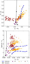 |
Fig. 1 NIR (top) and optical-NIR (bottom) colours for the three classes of objects considered in this work, using Euclid filters. Black solid lines display quasars in the redshift domains captured by the filters, with redshifts indicated directly on the lines. Blue lines display galaxies at (1 ≤ z ≤ 2), susceptible to contaminating the quasar samples. MLT: stars M, triangles L, and diamonds T. For the M, L ,and T, the filled are z - YE and hollow are IE - YE. |
Quasar LF parameters.
2.2 The high-z quasar population
The statistical model of the quasar (QSO) population is based on a collection nQSO of SEDs (also referred to as spectral templates or templates) and a set of parameters θQSO describing the quasars’ properties. The spectral templates used in this paper are smoothed versions of the quasar composites presented in Bañados et al. (2016) and parametric SED models that accurately reproduce the observed optical and NIR colours of luminous type 1 quasars over a wide range of redshifts and luminosities from Temple et al. (2021). The parameters are the redshift, z, and the apparent magnitude in a reference band, which we choose to be the Euclid H band, denoted HE. This allows us to compute the expected fluxes in each band,  at the
  value of the parameter set given the i-th SED model. The QSO likelihood of the data given θQSO is defined as the mixture of multivariate densities in Eq. (3). For the purposes of our paper, we let the redshift vary in the range 7 ≤ z ≤ 12. We aim for a maximum redshift of 12 as the Euclid bands will cover up to the HE band, and the Lyman-alpha emission line stays in the JE band until z ≈ 12.
To characterise the prior distribution of high-z quasars, we adopted the double power law parametric luminosity function (LF) from Willott et al. (2010) and adjusted the parameters fit to Matsuoka et al. (2023):
 (7)
(7)
where M1450 is the quasar rest-frame absolute magnitude at λ = 1450 Å and Φ(M1450, z) is the number of quasars per magnitude bin, and unit volume at redshift, z. The parameters are the normalisation, Φ*, the break magnitude, M*1450, the bright end slope, β, and the faint end slope, α, their values can be found in Table 1. Using the apparent magnitude in the HE band, we can write the surface density of quasars in the sky in mag-1 × deg-2 × dz-1 units as
![Mathematical equation: \begin{align} \rho_\text{QSO}(H_E,z)=\dfrac{1}{4\pi}\times \dfrac{{\rm d}V_c}{{\rm d}z}\times \Phi \left[ H_{E} -\mu -K_{corr}(z),z \right], \end{align}](/articles/aa/full_html/2025/09/aa53654-25/aa53654-25-eq18.png) (8)
(8)
where
μ represents the distance modulus, defined as a function of the luminosity distance DL by
 (9)
(9)Kcorr(z) denotes the K-correction, which converts the absolute magnitude at rest-frame λ = 1450 Å into the observed H-band magnitude, and
 is the co-moving volume element per steradian and per redshift interval dz.
Figure 2 illustrates the number of quasars per redshift bin and up to three different values of HE across the entire 15 000 deg2 of the EWS, as derived from Eq. (8). This demonstrates that Euclid will detect tens of quasars brighter than HE ≈ 22.5 between redshifts 7 and 8, and potentially a few up to z ≈ 9. Up to this HE magnitude, the selection with Owl-z will be robust, while becoming increasingly more hazardous beyond it.
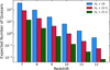 |
Fig. 2 Expected number of quasars per redshift bin in the 15 000 deg2 EWS given the high-z quasar LF adopted in this paper. In blue are shown the numbers of quasars expected up to HE < 24, in crimson with HE < 22.5 and in green with HE < 21.5. |
2.3 The MLT star population
For the purpose of our Bayesian analysis, we need to model the spatial distribution of MLT dwarfs, along with their luminosity and spectral energy distributions from the optical to the NIR. For spectral energy distributions, we used the stellar dwarf Luyten Half-Second (LHS) library (Bakos et al. 2002) for M3-M5 brown dwarfs and the brown dwarf spectral library SpeX prism (Burgasser 2014; Burgasser & Splat Development Team 2017) for other spectral types. The use of spectral data enables magnitudes and colours to be correctly determined and modelled in the Euclid filters or any other filters as long as they overlap the spectral range of the spectra. Moreover, there are between 5 and ≈50 spectra available for each spectral type. Our models also include WISE photometric data for the W1 and W2 bands, anchored to the average JHK photometry of brown dwarfs as tabulated in Best et al. (2017). This allows us to include in our model the WISE photometry that cannot be calculated from the MLT spectra that do not extend beyond the K band. In Fig. 3, we show the W1 - W2 colours for all MLT types as indicated in Best et al. (2017), indicating that T dwarfs, especially late types, have very strong W 1 - W2 colours that can easily be discriminated from the colours of high-z quasars.
To estimate the probability of brown dwarf contamination when searching for high redshift objects in wide-field imaging datasets, the spatial distribution of stellar dwarfs in the Galaxy is usually modelled and restricted to the thin disc of the Milky Way (Caballero et al. 2008; Euclid Collaboration: Barnett et al. 2019; Pipien et al. 2018b). A detailed modelling of the thin disc is beyond the scope of this paper, therefore, we followed Caballero et al. (2008) by assuming a similar thin-disc scale height for LT dwarfs to its value determined from earlier stellar dwarf types (GKM) and a simplified exponential vertical and horizontal distribution. For a detailed theoretical modelling of thin disc parameters as a function of stellar age and metallicity, calibrated against Gaia and APOGEE data, we refer, for example, to Sysoliatina & Just (2022).
At the magnitudes corresponding to the depth of the EWS (~24), the distance to T dwarfs varies from ~150 pc for the coldest to ~450 pc for the hottest. With a scale height of the thin disc of the order of 300 pc (Gaia Collaboration 2023; Vieira et al. 2022), we infer that the sole thin disc approximation will reasonably well represent the population of T dwarfs detectable in the EWS. However, the same will not be true for M dwarfs. An M6 dwarf at an apparent magnitude HE ≈ 24 is at a distance of ~4000 pc, extending well beyond the thin disc into the thick disc or the halo. As a matter of fact, the JWST has revealed in extragalactic fields a significant number of extremely faint and low-temperature brown dwarfs extending well into the thick disc and possibly into the halo, at distances of up to 2 kpc (Hainline et al. 2024b,a; Burgasser et al. 2024). An analysis of the thick disc contamination is therefore warranted.
For this analysis, we followed a similar approach to that used in Ryan & Reid (2016) and compared the distribution of stellar dwarfs in thin and thick discs as a function of magnitude. We adopted a value of 330 pc for the scale height of the thin disc (Caballero et al. 2008), 800 pc for the scale height of the thick disc (Vieira et al. 2023), and 2250 pc (Caballero et al. 2008) for the value of the scale length of both discs, along with a normalisation factor between the thick and thin disc local densities of 10%. Using Eq. (12) of Pipien et al. (2018b), we compared brown dwarf densities for different spectral types in the thin and thick discs for two lines of sight: b = 90° and (l, b) = (90°, 30°) (the lowest Galactic latitude of the EWS is b = 23°). For local volume densities in the Galactic plane and absolute Euclid magnitudes by spectral type, we refer to Table 2 of Euclid Collaboration: Barnett et al. (2019) and the references therein (Dupuy & Liu 2012; Skrzypek et al. 2016; Bochanski et al. 2010). Late-type M dwarfs can potentially contaminate searches for galaxies or quasars at high redshift in some surveys; however, as we discuss later in this paper, only L and T-type brown dwarfs contaminate the search for z ≥ 7 with Euclid. Consequently, for the purposes of this work, we restricted our analysis to the brown dwarf population within the M dwarf population, that is, dwarfs of a type later than approximately M6.
The analysis (see Fig. 4) indicates that up to Euclid magnitude HE ~ 24, the thin disc dominates the number of L and T dwarfs at low and high Galactic latitudes. For M6 to M9 dwarfs, the thick disc is the main contributor above H ~ 22.5 magnitudes at high Galactic latitudes, whereas at low Galactic latitudes, the thin disc dominates up to HE ~ 24.5 and beyond.
For the purposes of our paper, Galactic latitude is, therefore, the dominant parameter affecting the population of contaminating stars. We explore the effect of Galactic latitude on the performance of our code in Sect. 4.
This simple analysis assumes that stellar dwarf populations are the same in both thin and thick discs. This oversimplification ignores the differences in age and metallicity between the constituents of the thin and thick discs and, therefore, the significant differences that may exist between the stellar dwarf populations within them. Early M-type dwarfs (M0 to M5) have masses above the hydrogen-burning minimum mass and their luminosity evolves little on time scales up to 10 billion years, whereas brown dwarfs below this limit cool on much faster time scales (Reid 2013). As a result, late M-type dwarfs evolve into later spectral types and their luminosities drop rapidly over timescales of a Gyr or less. The thick disc, which is older than the thin disc, should therefore be depleted of late-type brown dwarfs (M6 to M9 and L), and T dwarfs should be significantly less luminous in the thick disc than in the thin disc (see also the discussion in Caballero et al. 2008). This suggests that the stellar densities reported in Fig. 4 are likely to be seriously overestimated in the thick disc at a given magnitude for spectral types later than M5.
In conclusion, we restricted the modelling of the Galaxy’s brown dwarf population to the thin disc and analysed the impact of stellar density through its dependence on Galactic latitude. In the coming years, Euclid and JWST data will enable a more detailed understanding of the relative populations of brown dwarfs in the thin and thick discs.
We return to the formulation of our Bayesian model for the description of the stellar dwarf population. The parameters of this population are magnitude (or heliocentric distance), and spectral type {HE, spt}. We use the Euclid HE band as the reference band for calculating magnitudes and the spectral types from M6 to T9. Using the notation described in Sect. 2, we can express the weighted evidence of this population as follows:
 (10)
(10)
where ρs(Hmod, spt) is the surface density of the contaminating brown dwarf population of Euclid magnitude, Hmod, and spectral type, spt, at a given Galactic longitude, l and latitude, b. We model the spatial distribution across the Galaxy in mag-1 × deg-2 × spt-1 units as a function of the heliocentric distance to the star, d, assumed to be far smaller than the solar galactocentric distance, R⊙ (Caballero et al. 2008):
 (11)
(11)
where,
![Mathematical equation: \mathcal{R}(d_{H_{mod}},l,b)=\exp \left[{-d_{H_{mod}}\left(-\frac{\cos(b)\cos(l)}{h_{R}}\pm \frac{\sin(b)}{h_{Z}}\right)}\right]](/articles/aa/full_html/2025/09/aa53654-25/aa53654-25-eq23.png) (12)
(12)
where  is the local volume density of brown dwarfs of spectral type spt, Z⊙ the height of the Sun above the Galactic plane (assumed to be 27 pc), hZ and hR the scale height and length of the thin disc as mentioned above, and the sign convention indicates whether the source is above or below the Galactic plane (see Caballero et al. 2008). Finally, Hmod and dHmod are related via
 (13)
(13)
where Hmod and MHmod are the apparent and absolute magnitudes in the reference band, HE, and E(B - V) is the interstellar reddening.
Using the modelling of the high-z quasar population (Sect. 2.2) and the MLT population described in this section (M6 to T9), we derive the ratio of the brown dwarf to high-z QSO density on the Euclid footprint. This is shown in Fig. 5 for two different apparent magnitudes. Figure 6 shows the densities of quasars and M6 to T9 brown dwarfs for two positions with different Galactic coordinates in the Euclid footprint.
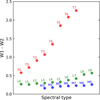 |
Fig. 3 WISE W1 - W2 colours of MLT dwarfs from Best et al. (2017) shown in blue, green, and red, respectively, with the values indicating their spectral type. |
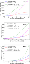 |
Fig. 4 Brown dwarf number counts as a function of H-band magnitude for the thin and thick discs in two different field locations (b = 90° and (l,b)=(90°,30°)). Top: M6 to M9 spectral types, middle: L0 to L9 and bottom: T0 to T8. |
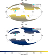 |
Fig. 5 Ratio of the surface density of brown dwarfs of spectral type M6 to T8 to the surface density of z > 7 quasars over the Euclid footprint shown in Galactic coordinates and galactic projection. Top: for magnitude HE = 20. Bottom: for magnitude HE = 24. |
2.4 The contaminant galaxy model
There are two different types of galaxies susceptible to contaminating the quasar samples because they display red colours that mimic those of high-z quasars, particularly at low S/N: early-type galaxies at intermediate redshift (1 < z < 2) on the one hand and dusty star-burst galaxies on the other hand. The former exhibit an important 4000 Å break because they are dominated by an old stellar population, whereas the presence of dust reddens the latter. To assess the extent of this contamination by intermediate- z galaxies, we have carried out two different tests. The first one consists of precisely determining the contaminant population by using straightforward simulations. The second one is to quantify the contamination in the real Universe based on the COSMOS2022 field (Weaver et al. 2022) by computing the LF of the contaminant population. The LF will be used later to model the abundance of contaminant galaxies.
To precisely identify the contaminant population, we ran Owl-z on a simulated catalogue containing 100 000 galaxies uniformly sorted in redshift ( 0 ≤ z ≤ 6), spectro-photometic templates, and extinction values (between 0 ≤ AV ≤ 3 magnitudes), using the Calzetti extinction law (Calzetti et al. 2000). The simulated catalogue was generated using make_catalogue, a tool from the HyperZ tool (Bolzonella et al. 2000). The template library includes two evolutionary synthesis models: (1) a delta burst based on a single stellar population (SSP) model from the Bruzual & Charlot code (Bruzual & Charlot 2003), with a Chabrier IMF (Chabrier 2003), assuming solar metallicity; and (2) ten Starbursts99 templates (Leitherer et al. 1999), including emission lines, for single bursts and constant star formation rate models, each one spanning five metallicities (Z = 0.04, 0.02, 0.008, 0.004, and 0.001), and 37 ages for the stellar population (between 0 and 1 Gyr). Apparent magnitudes and associated errors have been computed using these templates, sorted to uniformly sample the range of magnitudes where galaxies are expected to be the dominant population in the EWS, in the reference HE-band, that is 22 ≤ HE ≤ 25. Photometric error bars and noise are scaled to apparent magnitudes, assuming a Gaussian distribution, according to the expected S/N in the different bands used in the EWS. The probability threshold for the selection as a quasar is set to Pq = 0.1 for this analysis, following Mortlock et al. (2012) and Euclid Collaboration: Barnett et al. (2019).
The first result of this experiment is that young starbursts, represented by the Starburst99 models, only contaminate the sample at low S/N values for extremely high values of AV ≥ 1.5, spanning a relatively broad domain in redshift (1 ≤ z ≤ 5). It is important to acknowledge the significant influence of S/N values in the reference magnitude on our selection process. Indeed, a low S/N in the reference filter H induces a noisy determination of the J - H colour, which, in turn, leads to a higher degree of confusion in the probability calculation and a greater likelihood of misidentifying high-z quasars. This is a general remark affecting all contaminant galaxies but is particularly important for dusty starbursts. The main contaminants among this population are galaxies at z ≳ 4 with AV ≥ 1.5, and galaxies at 1 ≤ z ≤ 2 with AV ≥ 3. In the two cases, such extremely reddened galaxies are relatively rare in the real Universe at these redshifts.
Our analysis shows that the main contamination comes from early-type galaxies, represented by SSP models, with ages above 1 Gyr, at intermediate redshifts, 1 < z < 2. Indeed, the spectral energy distribution of early-type galaxies, such as elliptical and lenticular galaxies, is characterised by an old stellar population, well represented by an initial burst of star formation followed by a rapid decline (see e.g. Ali et al. 2024). Contrary to dusty starbursts, these galaxies are relatively abundant at 1 < z < 2. For this reason, in the following, we consider that the main contamination comes from early-type galaxies. In this regard, our results are consistent with the assumptions of previous works (e.g. Euclid Collaboration: Barnett et al. 2019). The abundance of these galaxies has been well studied at z ~ 1.5, for instance, by Zucca et al. (2006), who studied the evolution of the LF for different filters and spectrophotometric types of galaxies. We can use these previous findings to guide our modelling in the sensitive magnitude domain, as shown below.
After identifying the nature of the contaminant galaxies, we determine the LF of this population. For this need, we use the Euclidised COSMOS2022 catalogue (Weaver et al. 2022), named E-COSMOS hereafter. This catalogue is described in more detail in Sect. 4.3.3. Note that for galaxies detected in the JE-band at intermediate redshift, the relevant filter for determining the LF is the rest-frame B band.
To represent the LF, we use the classical parameterisation provided by the Schechter function (Schechter 1978) in terms of magnitude given by:
![Mathematical equation: n(M)=(0.4\ \ln 10)\ \phi ^{*}\ [10^{0.4(M^{*}-M)}]^{\alpha +1}\exp[-10^{0.4(M^{*}-M)}].](/articles/aa/full_html/2025/09/aa53654-25/aa53654-25-eq26.png) (14)
(14)
Here, n(M) dM represents the number of galaxies per comoving Mpc3 with magnitudes between M and M + dM. The parameters are as follows:
φ*: the normalisation factor, representing the overall volume density of galaxies in Mpc-3 × mag-1.
M*: the characteristic magnitude represents the cut-off between the (bright) luminosity regime dominated by the exponential function and the (faint) regime dominated by the power-law.
α: the faint-end slope of the LF, describing the distribution of the faintest galaxies.
For the sake of consistency, before selecting the target population of contaminant galaxies in E-COSMOS, we run Owl-z on the ECOSMOS catalogue, with only one contamination source: MLT stars, and the same threshold as before for the selection of high-z quasars. We checked the spectrophotometric type and redshift of the 16 galaxies that have been selected as quasars. They are all early-type galaxies at intermediate redshift (z ~ 1.5), as expected from previous simulations.
To model the LF for this population of contaminants, we used the E-COSMOS catalogue to extract the subset of early-type galaxies within the sensitive redshift domain 1 < z < 2. To compute absolute magnitudes, we model the spectral energy distribution with a template well suited to represent this population, namely a short, exponentially decaying model with characteristic star-formation time τ = 0.1 Gyr, age = 10 Gyr and solar metal-licity (Z = 0.02). It is worth mentioning that the precise choice of this model does not affect the results. The LF points and their associated error bars were then computed; error bars in the LF include Poisson noise and field-to-field variance. Field-to-field variance is derived using the Trenti & Stiavelli method and calculator (Trenti & Stiavelli 2008). We then fit the data points with the Schechter function in Eq. (14) using a χ2 minimisation.
Towards the faint end, we applied a magnitude cut to MB < -19.7 because beyond this limit, our sample suffers from incompleteness. The parameters were chosen to enable easy comparison with the work of Zucca et al. (2006). This motivated us to fix the same value for the parameter α. For comparison, a value of α = 1.0 gives a similar result to the function adopted by Euclid Collaboration: Barnett et al. (2019) to represent the same population. We note that the precise choice of α is irrelevant here because, on the one hand, only the faintest part of the LF is dominated by the power law and, on the other hand, the population of contaminant galaxies lies preferentially in the bright end.
Fig. 7 shows that our LF points are in good agreement with Zucca et al. (2006). Our fit parameters are shown in Table 2. The LF obtained above is then used to model the prior distribution of early-type galaxies ρgi (Hmod, z) given in mag-1 × deg-2 × dz-1 units by:
![Mathematical equation: \begin{align} \rho_g(H, z_g) = \dfrac{1}{4\pi} \times \dfrac{{\rm d}V_c}{{\rm d}z_g} \times \Phi_g \left[ H_{\text{mod}} - \mu - K_{\text{corr}}(z_g), z_g \right]\text{,}\end{align}](/articles/aa/full_html/2025/09/aa53654-25/aa53654-25-eq27.png) (15)
(15)
where zg is the redshift range of the contaminant galaxies 1 < z < 2 and Φg is the LF fit obtained in this work.
For a given set of parameters, {zg, Hmod}, and an early-type galaxy model, gi, the weighted evidence can be quantified as
 (16)
(16)
Figure 8 displays a comparison between the surface number density of early-type galaxies in the 1 < z < 2 interval and z > 7 quasars as a function of apparent magnitude. The population of contaminant galaxies clearly dominates the number counts.
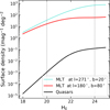 |
Fig. 6 Surface number densities of MLT stars compared to z > 7 quasars, as a function of apparent magnitude, in two different locations of the Euclid footprint. |
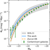 |
Fig. 7 LF fit in the B-band (blue) in addition to its 95% confidence interval (grey) for the population of early-type galaxies at 1 < z < 2 in the E-COSMOS catalogue data (green), compared to the early-type galaxies (dashed orange) LF fit by Zucca et al. (2006). |
3 Technical description of Owl-z
The Owl-z code calculates the probability of each preselected candidate belonging to one of the modelled populations, namely high-z quasars, early-type galaxies at intermediate redshifts, and MLT dwarfs. The code is self-contained and written in the Python programming language and its various packages, such as NumPy, SciPy, and Astropy. It is capable of functioning without any dependencies on external software.
Comparison of the Schechter function parameters.
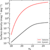 |
Fig. 8 Surface number density of early-type galaxies integrated in the redshift interval 1 < z < 2 compared to the quasars surface number density integrated over the redshift interval 7 < z < 12 quasars, as a function of apparent magnitude. |
3.1 Inputs
The Owl-z code relies on the computation of colours from the SEDs for all three populations in addition to the K-corrections for quasars and galaxies. To do so, the model requires the filter transmission curve data for each band, as well as a designated reference magnitude. Additional parameters are the magnitude range and the redshift range to explore, for each population. In the case of brown dwarfs, for each spectral type, the range of absolute magnitudes and the local densities should be provided. Templates for each population should be provided, and the code distribution already includes a large number of them for the three populations considered. It is possible to add as many templates as required, provided that they are in the correct format.
3.2 Outputs
The programme provides a list of probabilities of belonging to each class for each source. The user then interprets the data and makes a decision by comparing these probabilities with a threshold, ζ. Furthermore, it provides a list of useful output parameters, including the optimal redshift for galaxies and quasars and the optimal spectral type for the best-fit stellar model. It also provides the SEDs of the galaxies and quasars that provide the maximum posterior condition. Note that the ‘best-fit’ output of a Bayesian code is the ‘maximum posterior’ (MAP), calculated by maximising the posterior, that is max(wq), where  are given by
 (17)
(17)
In the following sections, we use the terms best-fit or MAP, but we always refer to the same Bayesian definition above.
Known quasars at z > 7.
3.3 Efficiency
Owl-z has several efficiency indicators:
Owl-z requires the user to fill a configuration file which is straightforward to modify, requiring only the input of the user to enable its operation.
The code is self-sustained, whereby the models and K-corrections are calculated concurrently with the code and the input parameters.
The code is flexible regarding the numbers and nature of bands used, provided that they do not overlap.
The code is written with high-performance computing methods in mind and is partly written in Cython for the purpose of enhancing numerical speed.
In addition to providing a probability value, the model also provides additional output parameters for each source, thus facilitating a more accurate interpretation of the results.
3.4 Limitations
A natural limitation of the code is that the filters correspond to the spectral range of the templates used, for brown dwarfs on the one hand and for galaxies and quasars in the redshift ranges to be explored for each of them.
In the released version of the code corresponding to the one described in this paper, the brown dwarf templates are observed spectra and cover up to 2500 nm, thus imposing that the filters that can be provided are limited to the K-band. The galaxy and quasar templates have a sufficient spectral range for the redshift ranges explored in this paper and do not impose additional limits.
As will be seen later in this paper, in Sect. 4.2, the colours in the WISE filters have been used to further model the SED beyond the K-band, but this is exclusively possible with the tabulated data provided in Best et al. (2017) and used in the code and cannot be generalised to other datasets extending beyond K-band. Extending the filters that can be used beyond the K-band would require brown dwarf templates with extended spectral ranges that are not readily available.
4 Validation and performance
4.1 Methodology
This section is dedicated to the validation of Owl-z using two different approaches. The first one consists of re-identifying all the z > 7 spectroscopically confirmed quasars available in the literature. To achieve this, Owl-z was configured on a case-by-case basis with the photometric data from which the individual quasars were identified. The second approach relies on simulating different flavours of the EWS catalogues, allowing us to quantitatively evaluate the performance expected for Owl-z based on the measurement of the completeness, a measurement of how many (if any) quasars we misidentify with this process and purity, a measurement enables us to ascertain whether we are still contaminated among the objects identified as quasars by Owl-z. A global performance metric is also introduced, combining both completeness and purity. Performance estimators are important for optimising the selection of high-z quasar candidates with Owl-z, minimising the demand for spectroscopic follow-up and maximising the confirmation rate with a reasonable observational effort.
4.2 Re-identifying known z > 7 quasars
We analyse the performance of our code in recovering known and spectroscopically-confirmed quasars at z > 7 and selected from near-IR surveys. The versatility of Owl-z allows us to apply it to the different optical and NIR data sets used in the discovery of these quasars. The objective here is to determine if Owl-z is able to identify them as quasars and to compare their spectroscopic redshift with the redshift obtained by the code.
Table 3 lists the quasars used for this analysis, the photometric bands used for their discovery, their measured spectroscopic redshifts, and their reference magnitude.
The photometric data, different for each quasar, include z-band data (zDECam) from DECaLS (Dey et al. 2019), z- and y-band data (zPS1 and yPS1) from The Pan-STARRS1 Surveys (Chambers et al. 2016), g-, r-, i-, z-, and y-band data (gHSC rHSC, iHSC, zHSC, yHSC) from Subaru/HSC and Y-, J-, H-and K-band data from UKIDSS (Warren et al. 2007). Data from WISE (Wright et al. 2010) were also used. Given the shallow depth and non-constraining photometry in the W3 and W4 bands, we only use photometric data from the W1 and W2 bands in the following.
The pre-selection methods used to select these quasars were mainly based on colour selection and the identification of strong Lyman breaks (z - J > 4) around ~1μm. An additional criterion was used for the five cases out of eight where WISE photometry was available, consisting of a W1 - W2 < 0.7 colour selection enabling the rejection contamination by T-dwarfs (see Fig. 3).
The results of Owl-z are also presented in Table 3, in particular, the output redshifts and Pq values returned by the code. As further discussed in Sect. 4.3.2, the Owl-z output redshifts are in good agreement with the actual redshift of the objects. The primary potential contaminants expected for the QSOs in this study are L brown dwarfs. Owl-z yields probability Pq > 0.99 for all of the QSOs above, showing the high performance of the code in re-identifying the whole sample. Fig. 9 shows the photometric data, including error bars, for all quasars and the best-fit quasar and MLT dwarf solutions returned by the code.
Some results deserve a specific comment. Owl-z has provided an excellent result for all quasars, including those detected in a single band with non-detection constraints in the others (J2356+0017 and J1243+0100) because the photometric bands in HSC are very deep, and the Lyα break much easier to detect. These quasars have broad Lyα emission and are low-luminosity quasars, matching well the properties of the quasar population model (Sect. 2.2), unlike the SEDs of the MLT dwarfs (Sect. 2.3). As expected, the best-fit MLT solutions for quasars with WISE photometry are late M or L dwarfs, given the aforementioned colour selection criterion (W1 - W2 < 0.7) that excludes T dwarfs from photometric selection (Fig. 3).
To assess the impact of WISE data on the performance of Owl-z, we conducted an experiment in which WISE data were removed from the selection process. The results indicate that WISE data were crucial only in identifying one quasar, J0252-0503. Without WISE data, J0252-0503 would have been misclassified as a T star. For the remaining candidates, the exclusion of WISE data primarily led to a decrease in selection probability for the quasar J0313-1806, while the probability for candidates J0038–1527, J1342+0928 and J1007+2115 remained very high (see Table 3).
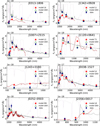 |
Fig. 9 Photometric data for the eight spectroscopically confirmed quasars at z > 7 and the Owl-z best-fit solutions for quasars and MLT dwarfs. The original photometric data points are represented by blue squares. The best-fit quasar model is in dashed grey, the best-fit model for an MLT dwarf is in dashed brown, and the filter transmission curves are shown in solid light purple. Model photometry for best-fit solutions is represented by green triangles for quasars and red stars for MLT dwarfs. |
Used bands characteristics.
4.3 Expected performance on EWS simulated data
The performance of Owl-z on the EWS is estimated in terms of completeness and purity in order to ascertain the sensitivity to confusion and contamination by MLT dwarfs and early-type galaxies. To this end, a series of catalogues is simulated in the following sections using Euclid filters (optical IE and NIR YEJEHE) and sensitivities detailed in Table 4.
4.3.1 Performance: Completeness
To estimate the completeness of the Owl-z selection method, we created a mock catalogue of 500 000 quasars. To gain a deeper understanding of the impact of using only Euclid data and of replacing or supplementing the existing data with other bands, three different scenarios have been developed. The first scenario involves using only Euclid data. In the second scenario, the optical band IE is replaced by the optical z-band of LSST. In the third scenario, in addition to the Euclid optical and NIR data, the photometry is extended to the WISE coverage in the W1 and W2 bands (see Table 5). The sensitivities of these additional bands can also be found in Table 4. The completeness is calculated on the EWS DR6 (Euclid Collaboration: Scaramella 2022) footprint, which covers 15 000 deg2. Quasars are randomly selected with a flat distribution in redshift in the range 7 ≤ z ≤ 12, a flat distribution in absolute magnitude M1450 in the range -29 ≤ M1450 ≤ -22, a flat distribution over all the SEDs in our library, and finally, a flat spatial distribution within the 15 000 deg2 of the EWS footprint. For each object in the catalogue, we calculate apparent magnitudes in the Euclid bands, in the LSST z-band, and in the WISE W1 and W2 bands. For photometric errors, we adopted those corresponding to the DR1 release of the LSST data (Ivezić et al. 2019) and those for the WISE data; we used the W1 and W2 bands and their corresponding errors from the survey description1. For Euclid photometric errors, we used the S/N maps across the EWS footprint as described in Euclid Collaboration: Scaramella (2022). All of this information can be found in Table 4.
We define the completeness C of the samples selected by Owl-z as follows:
 (18)
(18)
where TP (true positive) is the number of quasars that have been successfully classified as high-z quasars, and FN (false negatives) is the number of quasars that have been incorrectly classified as contaminants. For the sake of consistency with other work, we define a successful classification when Pq > 0.1, and we will examine in Sect. 5 how a different definition affects the results.
For all the objects in our mock quasar catalogue, we calculate the probability Pq, Ps, and Pg that the quasar is identified as a quasar, star, and galaxy, respectively, as defined in Eq. (1). Additionally, the SEDs for each category that allow for a maximum posterior are retrieved.
Results are presented as a function of redshift and HE magnitude in Fig. 10, for a selection from Euclid’s IE YE JE HE data. The colours correspond to different increments of the completeness value. We also evaluate how completeness varies when the LSST z-band (top-hand panel in Fig. 10) and the WISE W1 and W2 bands (bottom-hand panel in Fig. 10) are added to the photometric dataset. This is represented by the dotted red contour lines corresponding to the completeness increments.
In addition to the global completeness maps, we show in Fig. 11 the fraction of quasars with Pq < 0.1, namely, quasars misclassified as MLT stars (left panel) or intermediate redshift galaxies (right panel), colour-coded by the percentage of quasars lost in the bin. These maps illustrate the regions of the parameter space where the selection is least complete and help characterise the dominant sources of contamination as a function of redshift and HE magnitude. As seen in this figure, at z ~ 7 - 8 misclassification as MLT stars dominates, whereas at higher redshifts (z ≥ 8), the incompleteness reflects the overlap between quasars and mid-z interlopers, increasing with HE magnitude.
To achieve maximum completeness, quasar magnitudes need to be 2–3 magnitudes brighter than the EWS detection limit, depending on the redshift. The closer to the detection limit, and therefore the lower the S/N, the greater the confusion between quasars and brown dwarfs or galaxies at intermediate redshifts, preventing reliable identification.
Between redshifts 7 and 8, completeness is lower than at higher redshift, up to HE ≈ 21, due to greater confusion with late-type dwarfs. Due to the strong increase in late-type dwarf flux in the reddest part of the optical band and the wide width of the Euclid IE band, any late-type dwarf will appear significantly fainter in the IE band than in any z-band image of comparable depth (see Fig. 1). As a result, z-band data from LSST or from the UNIONS survey2 provide significantly improved discrimination against L- and T- dwarfs (dashed red curves in the left-hand plot of Fig. 10).
Figure 10 also shows a loss in completeness around redshift 10 and between magnitudes 22 and 23 of HE , compared with its value at lower redshift values. We attribute this loss in completeness mainly to an increase in confusion with early-type galaxies as their colours are very similar (see Fig. 12).
Finally, the analysis of completeness, including WISE data (bottom panel in Fig. 10) shows no significant improvement, in contrast to the improvement mentioned in Sect. 4.2 for the re-identification of known quasars at high redshift. Only a modest improvement in the decrease of the confusion with late-type dwarfs is perceptible for the brightest quasars at the lowest redshift. This is due to the fact that the depth of the WISE data (AB magnitude ~19 at 5σ in the W1 and W2 bands) does not match that of the Euclid data, making them unconstrained and allowing no significant improvements over the Euclid data alone, either above or below the WISE detection limit.
Scenarios explored in the simulations for the completeness estimation.
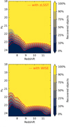 |
Fig. 10 Selection functions of high redshift quasars determined using Owl-z for Euclid IEYEJEHE data. The selection function designs the level of completeness per redshift bin; the completeness of a bin is calculated by counting the percentage of quasars in the bin with probability is Pq > 0.1. Several cases are shown: (top panel) In red, the optical band O of Euclid is replaced by the z-band from LSST. (bottom panel) Euclid IEYEJEHE data and in red Euclid IEYEJEHE in addition to WISE (W1 and W2 bands). |
4.3.2 Redshift estimation
Following Sect. 4.1, the redshift estimated by Owl-z corresponds to the maximum posterior value of the parameter z, that is, the maximum posterior  . We refer to it as ’photometric redshift’ (or zout hereafter).
The accuracy of the photometric redshift has been estimated by comparing the true redshift injected in the simulation ztrue to zout. Figure 13 displays this comparison for the redshift interval explored in the simulations presented in Sect. 4.3.1. To evaluate the accuracy of the photometric redshift, the sample has been limited to objects brighter than HE < 24, identified as quasars using the same criterion as in Sect. 4.3.1, that is, Pq > 0.1.
As shown in Fig. 13, an excellent correlation between ztrue and zout is found, irrespective of the photometric dataset. For the IEYEJEHE filter set, the Pearson correlation coefficient is found to be 0.97, whereas the Spearman correlation coefficient is 0.98, indicating a strong linear correlation. The same results are found for the zYEJEHE dataset. The classical quality estimators used for photometric redshift yield the following results, with ∆z = Zout - Ztrue: σ(∆z/(1 + z)) = 0.030, the median of (∆z/(1 + z)) = -0.007, and the normalised median absolute deviation, which is less sensitive to outliers: σz,MAD = 1.48 × median (|∆z|/(1 + z)) = 0.021. Regarding the fraction of outliers, defined in a conservative way as sources with ∆z > 0.1(1 + ztrue), it is found to be only 2.45% (2.23%) for the IEYEJEHE(zYEJEHE) datasets. Only 13.7% (13.3%) of the sample exhibit |∆z| > 0.05(1 + ztrue) for the IEYEJEHE(zYEJEHE) datasets.
These results demonstrate the quality and the reliability of the photometric redshift obtained by Owl-z for sources identified as high-z quasars. This is of utmost importance, given the use expected for the output redshift in the selection of samples for spectroscopic follow-up. It is also important in the determination of the purity, as discussed in Sect. 4.3.3.
4.3.3 Purity
The purity of the sample expresses the expected reliability of Owl-z in extracting true quasars from photometric observations of real fields, which is applied to the EWS in this particular case.
Here, we use the Euclid bands IE YEJEHE, the photometric depths and the variable S/N maps of Euclid.
We define the purity as
 (19)
(19)
that is, the number of true positive (TP) identifications divided by the total number of quasar identifications (TP + FP), where FP stands for false positives. With the above definition, a purity of 100% can either mean that no object( quasar or contaminant) has been identified as a quasar or all the identified objects are quasars. To estimate the purity, we need to simulate as accurately as possible the content of the input photometric catalogues, including the contaminant populations of stars and galaxies in a realistic way. Bright high-z quasars are rare, according to the current LF. For this reason, we force the inclusion of such sources in the simulated catalogues, as explained below, to determine how difficult it will be to identify and study these sources if they ever exist. In order to achieve this, the simulations are conducted on a surface that is ten times larger than that of the EWS. Subsequently, scaling back to the original surface (1000 deg2) is performed, whereby only those sources that the LF predicts are accounted for. We note that the definition of the purity as given above accounts for the possible detection of these unique, bright and rare quasars.
The COSMOS2020 field (Weaver et al. 2022) represents an ideal base for this exercise, given the extended wavelength coverage and the exceptionally good quality of the photometric redshifts that can be used as spectroscopic redshifts for our needs. All sources in this field have been fitted using LePHARE (Arnouts & Ilbert 2011) and a library of reference templates. This provided us with a best-fit template and a redshift. We used these results to compute the Euclid optical and NIR photometry via a process we call ‘Euclidisation’ (additional details will be provided in Euclid preparation, EC & Garnett et al.). This process has also allowed us to simulate the S/N and associated photometric errors in each filter. This new Euclid-like COSMOS catalogue will be called hereafter E-COSMOS.
The original COSMOS catalogue covers 2 deg2. To cover a statistically significant field of view, multiple realisations of the parent E-COSMOS catalogue are needed. This is done by randomly sorting the coordinates of the field centre within the EWS footprint in such a way that a full (not overlapping) large catalogue is created. This catalogue covers 1000 deg2 separated into six different areas. The rationale behind this choice is that it represents the smallest surface area over which we can account for a sufficient number of quasars. Furthermore, this surface has been divided across the region of interest in order to accommodate the various scenarios in galactic latitude and longitude, as well as to account for the inevitable differences in resolution, however slight they may be. Figure 14 and Table 6 display the location of these areas around the Euclid Footprint. It is worth noting that the location of the field is expected to have a direct impact on the performance, given the different distribution of contaminant stars on the one hand and the different S/N achieved across the EWS due to zodiacal light variations on the other hand (Euclid Collaboration: Scaramella 2022). These effects are discussed below. The E-COSMOS catalogue has been cleansed of all stellar objects and is situated at a considerable distance from the Galactic plane. To properly account for the presence of contaminant stars, we randomly inject additional MLT dwarfs into the catalogues, following the distribution presented in Sect. 2.3, reproducing the number densities expected at the galactic coordinates where the simulated field is located. Since E-COSMOS does not contain any spectroscopically identified high-z quasar, this population has been randomly injected in the simulated fields, following the prescriptions presented in Sect. 4.3.1 to properly account for the S/N in the EWS. High-z quasars are randomly sorted according to their LF. Obviously, the number of bright z > 7 quasars is expected to be very small in the EWS field. In particular, the current LF does not predict any quasar brighter than M1450 < -23 in the entire field. For these rare bright objects, if they exist, we force the measurement of the purity as explained above. To better capture this population, 10 realisations of the entire Euclid footprint are performed, allowing us to retrieve some quasars towards the brightest luminosities and up to redshifts z > 10. However, in order to facilitate consistent comparison of the statistical performance estimators C and P, it is necessary to normalise all populations to the same surface area (15 000 deg2).
Owl-z has been run on these simulated catalogues. The preselection criteria and Pq > 0.1 threshold applied are identical to those used for the completeness in Sect. 4.3.1. We study the variation of the purity as a function of redshift (zout) and apparent magnitude in the reference filter. The results presented in Fig. 15 provide a summary of the performance of Owl-z in terms of completeness and purity. In each bin, the figure displays the values of C and P. Additionally, it illustrates another performance estimator, the F-measure, which will be defined in Sect. 4.3.4. As shown in this figure, the code is expected to achieve a high purity for the brightest sources, irrespective of the redshift. The influence of the precise choice for the threshold in Pq is discussed in Sect. 5.1.
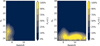 |
Fig. 11 Incompleteness maps of high-z quasar selection using Owl-z, shown as a function of redshift and HE -band magnitude. Each panel displays the fraction of quasars with Pq<0.1, i.e. quasars misclassified as MLT stars (left panel) or intermediate redshift galaxies (right panel), colour-coded by the percentage of quasars lost in the bin. These maps illustrate the regions of the parameter space where the selection is least complete and help characterise the dominant sources of contamination. |
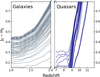 |
Fig. 12 Tracks of JE-HE colours as a function of redshift of early-type galaxies (left panel) and high redshift quasars (right panel). For the early-type galaxies, the lower the colour in the track, the younger the galaxy. |
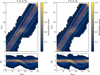 |
Fig. 13 Top: comparison between the true redshift and the redshift estimated by Owl-z with both Euclid IEYEJEHE dataset (left) and zYE JE HE dataset (right). Red solid lines display the 1:1 bisector; the thresholds corresponding to |∆z| > 0.1(1 + ztrue) and |∆z| > 0.05(1 + ztrue) are also displayed to guide the eye as orange dotted and white dashed lines, respectively. Bottom: residual ∆z = zout - ztrue as a function of redshift, with the red line corresponding to ∆z = 0. |
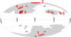 |
Fig. 14 Location of the regions of focus used in the computation of the purity how in Galactic coordinates and galactic projection (red). Details on these surfaces can be found in Table 6; the EWS DR6 footprint (grey). |
Properties of simulated areas and catalogues.
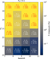 |
Fig. 15 Classification performance of Owl-z determined using the threshold ζ = 0.1, in each magnitude and redshift bin, N is the number of quasars in the bin, P is the purity, and C is the completeness. The colour code indicates the performance measurement F-measure in each bin |
4.3.4 Global performance
To evaluate the global performance of Owl-z by combining both the completeness and purity measurements, we introduce the F-measure, as follows:
 (20)
(20)
where P is the purity and C is the completeness, according to the definitions in Sects. 4.3.1 and 4.3.3, respectively. The F-measure is a statistical measurement employed to assess the performance of a classifier (Baeza-Yates & Ribeiro-Neto 2011).
The classification performance – specifically, the code’s ability to identify high-z quasars –is evaluated using the F-measure, which indicates the quality of the classification. A higher F-measure indicates a superior classification performance. Hereafter, we use F -measure as a performance metric.
The results summarising the performance of Owl-z in terms of F-measure are also provided in Fig. 15. As shown in this figure, high values of F-measure are obtained for bright (HE < 21) sources at all redshifts between 7 < z < 11, indicating that the performance in the spectroscopic confirmation of bright rare quasars is expected to be high. On the contrary, the F -measure drops significantly towards fainter magnitudes and high redshifts, following the drop in the purity value. We note that satisfying results can still be achieved for HE < 23 and z < 8. Also, the performance depends on the choice of the probability threshold, hereafter referred to as ζ, as discussed in Sect. 5.1.
To illustrate the effects of contamination, we show in Fig. 17 the contamination by galaxies (background colour) and indicate the relative fractions Ig of galaxies and Is of MLT stars among the contaminant population. Contamination is almost entirely dominated by galaxies, except in one redshift and magnitude bin where MLT stars also contribute. This is explained by the fact that the colours of MLT stars mainly contaminate the colours of quasars in the redshift bin [7-8] (see Fig. 1), and that the number of contaminants at high magnitudes are dominated by galaxies (see Figs. 5 and 8).
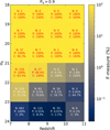 |
Fig. 16 Classification performance of Owl-z determined using the threshold ζ = 0.9, in each bin we report N: the number of quasars injected in the bin, P: the purity and C: the completeness. The colour code indicates the performance measurement F-measure in each bin. |
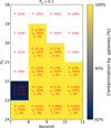 |
Fig. 17 Contamination by galaxies indicated by the colour map for the same quasar selection parameters as in Figure 15. The overlaid text indicates the purity of the quasars as in Figure 15 and the relative fractions of contamination by galaxies (Ig) and MLT stars (Is). |
5 Discussion
In this section, we study the influence of different parameters on the performance of Owl-z, such as the threshold used to select quasars as a function of redshift and magnitude. We also give some guidelines to optimise the selection of high-z quasars and their spectroscopic follow-up. The discussion in this section is based on the performance expected on the EWS.
5.1 Influence of the selection threshold
In the previous section, we discuss how we considered an object as a quasar candidate when the posterior probability, P, was above the threshold ζ = 0.1. This parameter clearly impacts the performance because lower values will improve the completeness while inducing worse purity values and vice-versa. There is a trade-off to find to optimise the performance. Here, we discuss the influence of ζ on F-measure.
To this end, we used the data discussed in Sect. 4.3.3, changed the value of ζ to select quasar candidates, and recalculated the F-measure in each bin. The results are presented in Fig. 15 for ζ = 0.1 and in Fig. 16 for ζ = 0.9. Two main trends are observed for sources brighter or fainter, respectively, than HE = 22. Increasing the threshold improves purity, albeit at the expense of completeness for faint sources (HE > 22). For bright sources (HE < 22), the completeness is almost unaffected by increasing the classification threshold, thanks to the ability of the code to compute high Pq values for bright quasars.
For faint sources, the performance of Owl-z drops rapidly towards the faintest magnitudes above HE = 22, irrespective of the redshift bin and ζ due to low S/N values, which contribute to a rapid decrease in purity, even when completeness is still good. The analysis of the results shows that early-type galaxies are the main contributors to contamination at these faint magnitudes (HE > 22). Conversely, at bright magnitudes (HE < 22 and brighter), the S/N is high and enables adequate classification between stars, galaxies, and quasars with good completeness, while higher values of ζ improve the purity and the values of the F-measure increase.
In Fig. 15, the 8 < z < 10 redshift bins for bright candidates (19 < HE < 22) are clearly affected by low purity values. The main sources of contamination in this area are early-type galaxies at redshifts 1 < z < 2 due to the confusion between the 4000 A break at intermediate redshift and the Lyman-α break at high redshift, as explained in Sect. 2.4. There is also a minor contribution from contamination by late L-type dwarfs. Increasing the classification threshold has the immediate effect of reducing this contamination and thereby improving the purity. As completeness remains high, this results in a significant improvement in F-measure values. This analysis suggests that an adaptive threshold can be used to optimise the F - measure values in the magnitude-redshift parameter space.
5.2 Optimising the identification of z > 7 quasars
We went on to investigate if the value of the F-measure can be further increased by adjusting the selection threshold ζ in each redshift and magnitude bin. To this end, we used the data discussed in Sect. 4.2, changed the value of ζ in increments of 0.1, and selected the value that maximises F in each bin. The result is summarised in Fig. 18, indicating the value of ζ that maximises F in each bin of magnitude, HE, and redshift, zout. The results show that for bright magnitudes (HE < 21), a low threshold value of ζ = 0.1 is sufficient to maximise F-measure. This is due to the robustness of the selection for high S/N values irrespective of the redshift, as shown previously. On the contrary, for faint magnitudes (HE > 21), the value of ζ needs to be increased to compensate for the decline in purity, requiring ζ values as high as 0.9 towards the faintest magnitudes.
In conclusion, adopting a variable threshold enables the optimisation of the F -measure and, consequently, the effectiveness of photometric and spectroscopic follow-up campaigns based on Owl-z selected candidates. Finding the best threshold value ζ for a quasar candidate with magnitude, HE, and a redshift, zout, from any other survey data can be done by following the same prescription presented in this article in the case of EWS.
5.3 Influence of the position in the EWS footprint
In this section, we evaluate the effect of different locations in the EWS footprint. As described in Euclid Collaboration: Scaramella (2022), different zodiacal light levels across the footprint modify the S/N for a given magnitude in each filter and different sky positions and Galactic coordinates introduce varying stellar densities, as described in Sect. 2.3. To this end, we selected six different regions in the Euclid footprint, representative of different zodiacal light levels and Galactic coordinates. These regions are shown in Fig. 14, and Table 6 lists their Galactic coordinates and S/N values at reference magnitudes in all Euclid filters.
According to the results presented in Sect. 4, the confusion by MLT dwarfs is only sensible in the redshift interval of z = [7,8], where there is also contamination by early-type galaxies. Therefore, we focussed the analysis on this redshift bin because it is more susceptible to being affected by the precise distribution assumed for MLT stars. In addition, this redshift bin is also the most populated by quasars, meaning that the results are expected to be statistically more significant than in the other bins. For each one of these regions, we compute simulated catalogues following the prescriptions in Sect. 4.3.3 and we ran Owl-z to derive the value of the F-measure.
The results are shown in Fig. 19 and display minor variations in the values of the F-measure. Regions 5 and 6 exhibit a slight decline in F-measure within the magnitude bin [21,22] compared to the others. This can be attributed either to the fact that these regions possess the lowest Galactic latitudes (b = 26 and b = 30) or to the most unfavourable S/N values. According to the results presented in Sect. 4, the comparison with region 3 (which is also at a low Galactic latitude, but has higher S/N values) suggests that S/N variation is the dominant factor in variations in F-measure. In other words, brown dwarf contamination does not appear to depend significantly on Galactic latitude within the Euclid footprint, which is consistent with Figure 4 and with the fact that up to magnitude ≈22 contamination is dominated by late-type L and T dwarfs at distances small compared to the scale height of the Galactic disc.
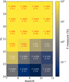 |
Fig. 18 Classification performance of Owl-z on the magnitude HE and redshift zout plane. The threshold value of ζ that maximises F-measure is given for each bin. |
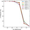 |
Fig. 19 F-measure evolution as a function of the HE magnitude in each of the regions shown in Table 6, computed in the 7 < z < 8 interval. |
5.4 Influence of thick-disc MLT
We aim to evaluate the robustness of our selection process when adding contamination from thick-disc MLTs that are not included in the model. We evaluate the impact on the F-measure of adding a contribution of thick-disc brown dwarfs to the input catalogue, following the prescriptions described in Section 4.3, and ignoring differences in brown dwarf populations between the thin and thick discs. To do so, we employ the density function outlined in Sect. 2 to generate a population of MLT dwarfs from the thick disc, in addition to the previously added MLT dwarfs from the thin disc, and we analyse the impact on F-measure on the six regions introduced previously. The results are presented in Fig. 20, comparing two scenarios: one where only thin-disc MLT dwarfs are injected in the input catalogue (shown by yellow lines) and another where thick-disc MLT dwarfs are added (shown by blue lines). The trends on these graphs can be qualitatively explained by the relative density of stars between the thin and thick discs as a function of magnitude. At low magnitudes, the thin disc dominates at all Galactic latitudes, and there are no differences between the two scenarios. At magnitudes above 21, however, and at high Galactic latitudes only (see Fig. 4), the thick-disc population begins to contribute to the counts and introduce a difference between the two scenarios (regions 1, 2, 4, and to a lesser extent region 3, which is at a relatively low Galactic latitude, but closest to the Galactic centre in longitude). Overall, this analysis serves as a sanity check in confirming that the precise modelling of the thick disc is unlikely to significantly affect the results for the EWS, but would be warranted for deeper surveys.
Figure 20 illustrates the drop in F-measure as more contaminants are introduced to the examined catalogues. These added contaminants are MLT stars drawn from the thick disc population, and have been introduced into all catalogues, including regions 2 and 1, which are the furthest from the Galactic plane. The Bayesian model cannot predict such MLT stars far from the galactic plane, as it only includes thin disc modelling (see Sect. 2.3). In regions 5 and 6, which are the closest to the Galactic plane, the Bayesian model expects a high number of contamination from MLT. Consequently, Owl-z does not classify MLT resembling QSO as QSO. However, when we move farther from the Galactic plane (regions 1, 2, and 4), additional contaminants that the model does not expect are encountered. As a result, they are more likely to be misclassified as a QSO, which in turn lowers the accuracy, namely, the F-measure of the Owl-z classification.
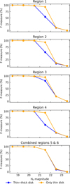 |
Fig. 20 F-measure evolution as a function of the HE magnitude in each of the regions shown in Table 6, computed in the 7 < z < 8 interval. Two cases are shown for the contribution of MLT stars. In yellow is presented the evolution when only the thin disc contribution is accounted for, both in the simulation and the Bayesian modelling. In blue, the same result is shown when the contribution of the thick disc is added to the simulations. |
5.5 Comparison with previous works
The results obtained in this article can be compared to previous similar works, at least qualitatively. A proper comparison will need to run the various codes on the same simulated catalogues, which is currently impossible because not all codes are publicly available. The Bayesian classification approach is similar to that adopted by Pipien et al. (2018b) for the analysis of the CFHQSIR survey (Pipien et al. 2018a) searching for quasars at 6.5 < z < 7.5. Our results in the lowest redshift bin are comparable to those of Pipien et al. (2018b). We note that Pipien et al. (2018b) did not include the population of contaminant galaxies, as this choice had no impact on their results because the dominant contamination in this bin comes mainly from LT stars, as shown in Sect. 4.
Our work also compares to and complements the study conducted by Euclid Collaboration: Barnett et al. (2019) on the EWS using a similar Bayesian classification method and the same contaminant populations of stars and galaxies. Although these approaches are comparable, our prior models and definitions of contaminant populations differ. Table 7 highlights the differences between the modelling of quasar and contaminant populations in these different studies. With respect to Euclid Collaboration: Barnett et al. (2019), the work with Owl-z extends the study beyond z > 9, and introduces different performance metrics in addition to the completeness, namely, the purity and F-measure (combining completeness and purity). Our definition of purity has also been adapted to account for rare quasars beyond z > 9 that could be found in the EWS if they ever exist. We also use updated prescriptions for the quasar LF and the contaminant populations. It is worth noting that here we have used the EWS S/N maps, making our predictions closer to the real observations. The performance of Owl-z in terms of completeness in the common redshift range with Euclid Collaboration: Barnett et al. (2019) is found to be better than in this previous work. The reason for this improvement is mainly the fact that the global S/N is expected to be better than assumed by Euclid Collaboration: Barnett et al. (2019). On the contrary, the effect of the detailed 2D modelling of the S/N in the EWS has little impact on the performance of Owl-z and similar codes, possibly because the depth is not dramatically different across the survey, as discussed in Sect. 5.3. Possibly the main advantage of Owl-z with respect to other existing codes is its versatility in adapting to different photometric surveys, as shown in Sect. 4.2. The code is meant to be publicly available and open to access.
6 Conclusions and perspectives
The conclusions of this work can be summarised as follows.
This work is intended as a reference article presenting Owl-z, a public Bayesian code aimed at identifying z > 7 quasars in massive photometric surveys. Owl-z is based on the classification of sources as high-z quasars or contaminants, with the latter being MLT stars or early-type galaxies at intermediate redshifts. The populations of contaminants have been carefully modelled for the needs of the Bayesian model selection. Although the code has been tuned to be used on the EWS, it can be easily adapted to different photometric surveys, as demonstrated in this work.
Owl-z has been able to re-identify all spectroscopically confirmed quasars at z > 7. This exercise has also demonstrated the versatility of Owl-z regarding its application to different photometric catalogues.
The performance of Owl-z based on F -measure, a metric combining completeness and purity, has been estimated using simulations for the EWS in a wide range of redshifts (7 < z < 12) and reference magnitudes (18 < HE < 24.5). The results show that Owl-z reaches its full performance for bright sources (HE < 22) irrespective of the redshift, meaning that the performance in the spectroscopic confirmation of bright rare quasars selected by Owl-z is expected to be high. The performance drops significantly towards fainter magnitudes and high redshifts.
The threshold value for the selection of quasars can be applied in the post-treatment phase, meaning that this value can be tuned to optimise the selection of z > 7 quasars. For instance, a small and large values can be used for the brightest and faintest sources (HE < 21 and > 21, respectively) to optimise the performance. Given the steep change of the optimum threshold on the magnitude versus redshift plane, a relatively crude cut on this plane could be adopted to optimise the spectroscopic follow-up.
A uniform performance is obtained with Owl-z across the EWS footprint, irrespective of the Galactic coordinates and relative S/N values.
The results of the code remain robust despite inevitable uncertainties in the detailed modelling of the contaminating stellar populations, in particular, the thin and thick discs.
The results obtained with Owl-z are promising and demonstrate its value as a flexible and robust tool for high-z quasar selection. However, several avenues can be explored to enhance its capabilities further and expand its applicability to upcoming large photometric surveys. These perspectives span both methodological improvements and broader scientific applications.
One major development direction involves extending Owl-z to additional photometric datasets, including those from LSST, Roman, and JWST. While the current implementation is tailored to Euclid-like data, its Bayesian framework is inherently adaptable. Nonetheless, brown dwarf spectral templates used in the model become unreliable beyond the K -band, highlighting the need to incorporate theoretical templates or real spectra from complementary instruments to maintain performance across varying wavelength ranges.
Integrating machine learning techniques into the classification pipeline offers another exciting prospect. Deep learning models, such as convolutional neural networks, could be used with Owl-z to refine candidate selection and optimise the balance between completeness and purity. This hybrid approach may prove especially effective at fainter magnitudes, where the performance of Owl-z currently diminishes.
In addition to the photometric selection methods employed in this study, the potential for utilising morphological information in classifying sources presents an intriguing avenue for future research. Incorporating morphological data could differentiate extended sources, such as early-type galaxies, from point sources such as high-z quasars. This classification, however, is contingent upon factors such as redshift and magnitude, as higher and elliptical redshift galaxies may appear increasingly compact due to resolution limits. While this work does not include a morphological analysis due to its complexity and the technical challenges associated with modelling Euclid detections of extended objects, we acknowledge that such an approach could significantly enhance the quasar selection process. Future studies could explore this integration, potentially refining our ability to mitigate contamination from non-quasar sources and improving the detection efficiency in the search for high-z quasars.
Additionally, improved modelling of contaminant populations is vital for maintaining selection accuracy in deeper surveys. Future works ought to consider a broader range of contaminants, including dusty star-forming galaxies, transients, and thick-disc brown dwarfs. These populations will likely become more prominent as surveys probe deeper into the high-z Universe.
Owl-z would also benefit from being embedded within a broader observational framework, including dedicated spectroscopic follow-up strategies. A systematic spectroscopic validation of candidates would refine the Bayesian thresholds and inform better post-selection filtering.
From a practical standpoint, future developments should also include optimising photometric preselection criteria to better handle systematic uncertainties and noise. This may involve simulation-based studies to understand the code’s response to varying observational conditions and tune selection thresholds accordingly. Moreover, cross-matching with multi-wavelength surveys (e.g. JWST, ground-based NIR observations) would add confidence to the classification of candidates and help eliminate artefacts or ambiguous detections.
Finally, although Owl-z was not originally designed for precise photometric redshift estimation, its outputs show potential in this area. Coupling Owl-z with dedicated redshift estimation tools in the post-processing stage could provide more accurate redshift predictions, further enriching its scientific utility.
Comparison of models, priors, and references used in various works.
Acknowledgements
This work makes use of publicly available data from the Euclid mission. We are grateful to members of the Euclid Science Working Group Primeval Universe, and in particular the Quasar Work Package, for their informal feedback and discussions during the development of this study. We would like to extend special thanks to Eduardo Bañados and Daniel Mortlock for their insightful input and collaboration. This research has also benefited from the use of quasar templates provided by Paul Hewett. We acknowledge Yo¯ suke Matsuoka, Feige Wang, and Jinyi Yang for kindly sharing spectra of quasars at z > 7. This research has made use of the Spanish Virtual Observatory project (https://svo.cab.inta-csic.es), funded by MCIN/AEI/10.13039/501100011033 through grant PID2020-112949GB-I00, particularly the SpeX Prism Library of brown dwarf spectral templates. We also acknowledge the use of the SVO Filter Profile Service “Carlos Rodrigo”, funded by the same grant. This research has been possible thanks to the computing facilities operated by CeSAM data centre at LAM, Marseille, France. Finally, we acknowledge the use of several open-source Python packages, including NumPy, SciPy, Astropy, Matplotlib, and Cython, which were instrumental in our data analysis and performance optimisation.
References
- Akeson, R., Armus, L., Bachelet, E., et al. 2019, arXiv e-prints [arXiv:1902.05569] [Google Scholar]
- Ali, S. S., De Propris, R., Chung, C., et al. 2024, ApJ, 966, 50 [Google Scholar]
- Arnouts, S., & Ilbert, O. 2011, Astrophysics Source Code Library [record ascl:1108.009] [Google Scholar]
- Bañados, E., Venemans, B. P., Morganson, E., et al. 2014, AJ, 148, 14 [Google Scholar]
- Bañados, E., Venemans, B. P., Decarli, R., et al. 2016, ApJS, 227, 11 [Google Scholar]
- Bañados, E., Venemans, B. P., Mazzucchelli, C., et al. 2018, Nature, 553, 473 [Google Scholar]
- Baeza-Yates, R., & Ribeiro-Neto, B. 2011, Modern Information Retrieval the Concepts and Technology Behind Search (New York: ACM Press) [Google Scholar]
- Bakos, G. Á., Sahu, K. C., & Németh, P. 2002, ApJS, 141, 187 [Google Scholar]
- Becker, G. D., Bolton, J. S., Madau, P., et al. 2015, MNRAS, 447, 3402 [Google Scholar]
- Belladitta, S., Moretti, A., Caccianiga, A., et al. 2020, A&A, 635, L7 [EDP Sciences] [Google Scholar]
- Bennett, J. S., Sijacki, D., Costa, T., Laporte, N., & Witten, C. 2024, MNRAS, 527, 1033 [Google Scholar]
- Best, W. M. J., Liu, M. C., Dupuy, T. J., & Magnier, E. A. 2017, ApJ, 843, L4 [NASA ADS] [CrossRef] [Google Scholar]
- Bochanski, J. J., Hawley, S. L., Covey, K. R., et al. 2010, AJ, 139, 2679 [NASA ADS] [CrossRef] [Google Scholar]
- Bolzonella, M., Miralles, J. M., & Pelló, R. 2000, A&A, 363, 476 [NASA ADS] [Google Scholar]
- Bosman, S. E. I., Davies, F. B., Becker, G. D., et al. 2022, MNRAS, 514, 55 [NASA ADS] [CrossRef] [Google Scholar]
- Bovy, J., Hogg, D. W., & Roweis, S. T. 2011, Annal. Appl. Stat., 5, 1657 [NASA ADS] [Google Scholar]
- Bruzual, G., & Charlot, S. 2003, MNRAS, 344, 1000 [NASA ADS] [CrossRef] [Google Scholar]
- Burgasser, A. J. 2014, ASI Conf. Ser., 11, 7 [Google Scholar]
- Burgasser, A. J., & Splat Development Team 2017, ASI Conf. Ser., 14, 7 [NASA ADS] [Google Scholar]
- Burgasser, A. J., Bezanson, R., Labbe, I., et al. 2024, ApJ, 962, 177 [NASA ADS] [CrossRef] [Google Scholar]
- Caballero, J. A., Burgasser, A. J., & Klement, R. 2008, A&A, 488, 181 [NASA ADS] [CrossRef] [EDP Sciences] [Google Scholar]
- Calzetti, D., Armus, L., Bohlin, R. C., et al. 2000, ApJ, 533, 682 [NASA ADS] [CrossRef] [Google Scholar]
- Chabrier, G. 2003, PASP, 115, 763 [Google Scholar]
- Chambers, K. C., Magnier, E. A., Metcalfe, N., et al. 2016, arXiv e-prints [arXiv:1612.05560] [Google Scholar]
- Dey, A., Schlegel, D. J., Lang, D., et al. 2019, AJ, 157, 168 [Google Scholar]
- Dupuy, T. J., & Liu, M. C. 2012, ApJS, 201, 19 [NASA ADS] [CrossRef] [Google Scholar]
- Euclid Collaboration (Barnett, R., et al.) 2019, A&A, 631, A85 [NASA ADS] [CrossRef] [EDP Sciences] [Google Scholar]
- Euclid Collaboration (Schirmer, M., et al.) 2022, A&A, 662, A92 [NASA ADS] [CrossRef] [EDP Sciences] [Google Scholar]
- Euclid Collaboration (Scaramella, R., et al.) 2022, A&A, 662, A112 [NASA ADS] [CrossRef] [EDP Sciences] [Google Scholar]
- Euclid Collaboration (van Mierlo, S. E., et al.) 2022, A&A, 666, A200 [NASA ADS] [CrossRef] [EDP Sciences] [Google Scholar]
- Euclid Collaboration (Mellier, Y., et al.) 2025, A&A, 697, A1 [Google Scholar]
- Fan, X., Strauss, M. A., Becker, R. H., et al. 2006, AJ, 132, 117 [NASA ADS] [CrossRef] [Google Scholar]
- Fan, X., Bañados, E., & Simcoe, R. A. 2023, ARA&A, 61, 373 [NASA ADS] [CrossRef] [Google Scholar]
- Gaia Collaboration (Recio-Blanco, A., et al.) 2023, A&A, 674, A38 [CrossRef] [EDP Sciences] [Google Scholar]
- Hainline, K. N., D’Eugenio, F., Sun, F., et al. 2024a, ApJ, 975, 31 [Google Scholar]
- Hainline, K. N., Helton, J. M., Johnson, B. D., et al. 2024b, ApJ, 964, 66 [Google Scholar]
- Hogg, D. W., Baldry, I. K., Blanton, M. R., & Eisenstein, D. J. 2002, arXiv e-prints [arXiv:astro-ph/0210394] [Google Scholar]
- Ivezić, Ž., Kahn, S. M., Tyson, J. A., et al. 2019, ApJ, 873, 111 [Google Scholar]
- Kang, Y., Hennawi, J. F., Schindler, J.-T., Tamanas, J., & Nanni, R. 2024, arXiv e-prints [arXiv:2412.03029] [Google Scholar]
- Laureijs, R., Amiaux, J., Arduini, S., et al. 2011, arXiv e-prints [arXiv:1110.3193] [Google Scholar]
- Leitherer, C., Schaerer, D., Goldader, J. D., et al. 1999, ApJS, 123, 3 [Google Scholar]
- Maiolino, R., Scholtz, J., Curtis-Lake, E., et al. 2024a, A&A, 691, A145 [NASA ADS] [CrossRef] [EDP Sciences] [Google Scholar]
- Maiolino, R., Scholtz, J., Witstok, J., et al. 2024b, Nature, 627, 59 [Google Scholar]
- Matsuoka, Y., Iwasawa, K., Onoue, M., et al. 2019a, ApJ, 883, 183 [Google Scholar]
- Matsuoka, Y., Onoue, M., Kashikawa, N., et al. 2019b, ApJ, 872, L2 [Google Scholar]
- Matsuoka, Y., Onoue, M., Iwasawa, K., et al. 2023, ApJ, 949, L42 [NASA ADS] [CrossRef] [Google Scholar]
- Mortlock, D. J., Warren, S. J., Venemans, B. P., et al. 2011, Nature, 474, 616 [Google Scholar]
- Mortlock, D. J., Patel, M., Warren, S. J., et al. 2012, MNRAS, 419, 390 [NASA ADS] [CrossRef] [Google Scholar]
- Nanni, R., Hennawi, J. F., Wang, F., et al. 2022, MNRAS, 515, 3224 [NASA ADS] [CrossRef] [Google Scholar]
- Oke, J. B., & Gunn, J. E. 1983, ApJ, 266, 713 [NASA ADS] [CrossRef] [Google Scholar]
- Pipien, S., Basa, S., Cuby, J. G., et al. 2018a, A&A, 616, A55 [NASA ADS] [CrossRef] [EDP Sciences] [Google Scholar]
- Pipien, S., Cuby, J. G., Basa, S., et al. 2018b, A&A, 617, A127 [NASA ADS] [CrossRef] [EDP Sciences] [Google Scholar]
- Reid, I. N. 2013, Brown Dwarfs, eds. T. D. Oswalt, & M. A. Barstow (Dordrecht: Springer Netherlands), 337 [Google Scholar]
- Robert, C. P. 2007, The Bayesian Choice: from Decision-theoretic Foundations to Computational Implementation, 2nd edn. (Berlin: Springer) [Google Scholar]
- Ryan, R. E. J., & Reid, I. N. 2016, AJ, 151, 92 [NASA ADS] [CrossRef] [Google Scholar]
- Schechter, P. 1978, The luminosity function for galaxies and the clustering of galaxies (Ann Arbor: University Microfilms) [Google Scholar]
- Scholtz, J., Witten, C., Laporte, N., et al. 2024, A&A, 687, A283 [NASA ADS] [CrossRef] [EDP Sciences] [Google Scholar]
- Skrzypek, N., Warren, S. J., & Faherty, J. K. 2016, A&A, 589, A49 [NASA ADS] [CrossRef] [EDP Sciences] [Google Scholar]
- Stern, D., Kirkpatrick, J. D., Allen, L. E., et al. 2007, ApJ, 663, 677 [NASA ADS] [CrossRef] [Google Scholar]
- Sysoliatina, K., & Just, A. 2022, A&A, 666, A130 [NASA ADS] [CrossRef] [EDP Sciences] [Google Scholar]
- Temple, M. J., Hewett, P. C., & Banerji, M. 2021, MNRAS, 508, 737 [NASA ADS] [CrossRef] [Google Scholar]
- Trenti, M., & Stiavelli, M. 2008, ApJ, 676, 767 [Google Scholar]
- Übler, H., Maiolino, R., Pérez-González, P. G., et al. 2024, MNRAS, 531, 355 [CrossRef] [Google Scholar]
- Vieira, K., Carraro, G., Korchagin, V., et al. 2022, ApJ, 932, 28 [NASA ADS] [CrossRef] [Google Scholar]
- Vieira, K., Korchagin, V., Carraro, G., & Lutsenko, A. 2023, Galaxies, 11, 77 [NASA ADS] [CrossRef] [Google Scholar]
- Wang, F., Yang, J., Fan, X., et al. 2018, ApJ, 869, L9 [NASA ADS] [CrossRef] [Google Scholar]
- Wang, F., Yang, J., Fan, X., et al. 2021, ApJ, 907, L1 [Google Scholar]
- Warren, S. J., Cross, N. J. G., Dye, S., et al. 2007, arXiv e-prints [arXiv:astro-ph/0703037] [Google Scholar]
- Weaver, J. R., Kauffmann, O. B., Ilbert, O., et al. 2022, ApJS, 258, 11 [NASA ADS] [CrossRef] [Google Scholar]
- Wenzl, L., Schindler, J.-T., Fan, X., et al. 2021, AJ, 162, 72 [NASA ADS] [CrossRef] [Google Scholar]
- Wilkins, S. M., Stanway, E. R., & Bremer, M. N. 2014, MNRAS, 439, 1038 [NASA ADS] [CrossRef] [Google Scholar]
- Willott, C. J., Delorme, P., Reylé, C., et al. 2010, AJ, 139, 906 [Google Scholar]
- Wright, E. L., Eisenhardt, P. R. M., Mainzer, A. K., et al. 2010, AJ, 140, 1868 [Google Scholar]
- Yang, J., Wang, F., Fan, X., et al. 2019, AJ, 157, 236 [Google Scholar]
- Yang, J., Wang, F., Fan, X., et al. 2020, ApJ, 897, L14 [Google Scholar]
- Zucca, E., Ilbert, O., Bardelli, S., et al. 2006, A&A, 455, 879 [CrossRef] [EDP Sciences] [Google Scholar]
All Tables
All Figures
|
Fig. 1 NIR (top) and optical-NIR (bottom) colours for the three classes of objects considered in this work, using Euclid filters. Black solid lines display quasars in the redshift domains captured by the filters, with redshifts indicated directly on the lines. Blue lines display galaxies at (1 ≤ z ≤ 2), susceptible to contaminating the quasar samples. MLT: stars M, triangles L, and diamonds T. For the M, L ,and T, the filled are z - YE and hollow are IE - YE. |
| In the text | |
|
Fig. 2 Expected number of quasars per redshift bin in the 15 000 deg2 EWS given the high-z quasar LF adopted in this paper. In blue are shown the numbers of quasars expected up to HE < 24, in crimson with HE < 22.5 and in green with HE < 21.5. |
| In the text | |
|
Fig. 3 WISE W1 - W2 colours of MLT dwarfs from Best et al. (2017) shown in blue, green, and red, respectively, with the values indicating their spectral type. |
| In the text | |
|
Fig. 4 Brown dwarf number counts as a function of H-band magnitude for the thin and thick discs in two different field locations (b = 90° and (l,b)=(90°,30°)). Top: M6 to M9 spectral types, middle: L0 to L9 and bottom: T0 to T8. |
| In the text | |
|
Fig. 5 Ratio of the surface density of brown dwarfs of spectral type M6 to T8 to the surface density of z > 7 quasars over the Euclid footprint shown in Galactic coordinates and galactic projection. Top: for magnitude HE = 20. Bottom: for magnitude HE = 24. |
| In the text | |
|
Fig. 6 Surface number densities of MLT stars compared to z > 7 quasars, as a function of apparent magnitude, in two different locations of the Euclid footprint. |
| In the text | |
|
Fig. 7 LF fit in the B-band (blue) in addition to its 95% confidence interval (grey) for the population of early-type galaxies at 1 < z < 2 in the E-COSMOS catalogue data (green), compared to the early-type galaxies (dashed orange) LF fit by Zucca et al. (2006). |
| In the text | |
|
Fig. 8 Surface number density of early-type galaxies integrated in the redshift interval 1 < z < 2 compared to the quasars surface number density integrated over the redshift interval 7 < z < 12 quasars, as a function of apparent magnitude. |
| In the text | |
|
Fig. 9 Photometric data for the eight spectroscopically confirmed quasars at z > 7 and the Owl-z best-fit solutions for quasars and MLT dwarfs. The original photometric data points are represented by blue squares. The best-fit quasar model is in dashed grey, the best-fit model for an MLT dwarf is in dashed brown, and the filter transmission curves are shown in solid light purple. Model photometry for best-fit solutions is represented by green triangles for quasars and red stars for MLT dwarfs. |
| In the text | |
|
Fig. 10 Selection functions of high redshift quasars determined using Owl-z for Euclid IEYEJEHE data. The selection function designs the level of completeness per redshift bin; the completeness of a bin is calculated by counting the percentage of quasars in the bin with probability is Pq > 0.1. Several cases are shown: (top panel) In red, the optical band O of Euclid is replaced by the z-band from LSST. (bottom panel) Euclid IEYEJEHE data and in red Euclid IEYEJEHE in addition to WISE (W1 and W2 bands). |
| In the text | |
|
Fig. 11 Incompleteness maps of high-z quasar selection using Owl-z, shown as a function of redshift and HE -band magnitude. Each panel displays the fraction of quasars with Pq<0.1, i.e. quasars misclassified as MLT stars (left panel) or intermediate redshift galaxies (right panel), colour-coded by the percentage of quasars lost in the bin. These maps illustrate the regions of the parameter space where the selection is least complete and help characterise the dominant sources of contamination. |
| In the text | |
|
Fig. 12 Tracks of JE-HE colours as a function of redshift of early-type galaxies (left panel) and high redshift quasars (right panel). For the early-type galaxies, the lower the colour in the track, the younger the galaxy. |
| In the text | |
|
Fig. 13 Top: comparison between the true redshift and the redshift estimated by Owl-z with both Euclid IEYEJEHE dataset (left) and zYE JE HE dataset (right). Red solid lines display the 1:1 bisector; the thresholds corresponding to |∆z| > 0.1(1 + ztrue) and |∆z| > 0.05(1 + ztrue) are also displayed to guide the eye as orange dotted and white dashed lines, respectively. Bottom: residual ∆z = zout - ztrue as a function of redshift, with the red line corresponding to ∆z = 0. |
| In the text | |
|
Fig. 14 Location of the regions of focus used in the computation of the purity how in Galactic coordinates and galactic projection (red). Details on these surfaces can be found in Table 6; the EWS DR6 footprint (grey). |
| In the text | |
|
Fig. 15 Classification performance of Owl-z determined using the threshold ζ = 0.1, in each magnitude and redshift bin, N is the number of quasars in the bin, P is the purity, and C is the completeness. The colour code indicates the performance measurement F-measure in each bin |
| In the text | |
|
Fig. 16 Classification performance of Owl-z determined using the threshold ζ = 0.9, in each bin we report N: the number of quasars injected in the bin, P: the purity and C: the completeness. The colour code indicates the performance measurement F-measure in each bin. |
| In the text | |
|
Fig. 17 Contamination by galaxies indicated by the colour map for the same quasar selection parameters as in Figure 15. The overlaid text indicates the purity of the quasars as in Figure 15 and the relative fractions of contamination by galaxies (Ig) and MLT stars (Is). |
| In the text | |
|
Fig. 18 Classification performance of Owl-z on the magnitude HE and redshift zout plane. The threshold value of ζ that maximises F-measure is given for each bin. |
| In the text | |
|
Fig. 19 F-measure evolution as a function of the HE magnitude in each of the regions shown in Table 6, computed in the 7 < z < 8 interval. |
| In the text | |
|
Fig. 20 F-measure evolution as a function of the HE magnitude in each of the regions shown in Table 6, computed in the 7 < z < 8 interval. Two cases are shown for the contribution of MLT stars. In yellow is presented the evolution when only the thin disc contribution is accounted for, both in the simulation and the Bayesian modelling. In blue, the same result is shown when the contribution of the thick disc is added to the simulations. |
| In the text | |
Current usage metrics show cumulative count of Article Views (full-text article views including HTML views, PDF and ePub downloads, according to the available data) and Abstracts Views on Vision4Press platform.
Data correspond to usage on the plateform after 2015. The current usage metrics is available 48-96 hours after online publication and is updated daily on week days.
Initial download of the metrics may take a while.