| Issue |
A&A
Volume 701, September 2025
|
|
|---|---|---|
| Article Number | A96 | |
| Number of page(s) | 16 | |
| Section | Catalogs and data | |
| DOI | https://doi.org/10.1051/0004-6361/202553739 | |
| Published online | 04 September 2025 | |
The hunt for new pulsating ultraluminous X-ray sources: A clustering approach
1
Department of Electronics, Information and Bioengineering, Politecnico di Milano,
via G. Ponzio, 34,
20133
Milan,
Italy
2
INAF–Osservatorio Astronomico di Roma,
via Frascati 33,
00078
Monte Porzio Catone,
Italy
3
Dipartimento di Fisica, Università degli Studi di Roma “Tor Vergata”,
via della Ricerca Scientifica 1,
00133
Roma,
Italy
4
INAF, Istituto di Astrofisica Spaziale e Fisica Cosmica,
Via Alfonso Corti 12,
20133
Milan,
Italy
5
Institut d’Estudis Espacials de Catalunya (IEEC), Edifici RDIT,
Campus UPC,
08860
Castelldefels (Barcelona),
Spain
6
Institute of Space Sciences (ICE, CSIC), Campus UAB,
Carrer de Magrans,
08193
Barcelona,
Spain
7
Ciela – Montreal Institute for Astrophysical Data Analysis and Machine Learning,
Montréal,
Canada
★ Corresponding author: This email address is being protected from spambots. You need JavaScript enabled to view it.
Received:
13
January
2025
Accepted:
19
July
2025
Abstract
Context. The discovery of fast and variable coherent signals in a handful of ultraluminous X-ray sources (ULXs) points to the presence of super-Eddington accreting neutron stars, drastically altering our understanding of the ULX class. Our capability of discovering pulsations in ULXs is limited, among other issues, by poor statistics. However, catalogues and archives of high-energy missions, such as XMM-Newton, Chandra, and Swift, contain information that is often overlooked, but could otherwise be used to identify new candidate pulsating ULXs (PULXs).
Aims. The goal of this research is to single out candidate PULXs among ULXs that have not shown pulsations due to an unfavourable combination of factors (low statistics, low pulsed fraction, etc.).
Methods. We applied an artificial intelligence approach to an updated database of ULXs detected by XMM-Newton. The sample counts 640 sources for a total of ~1800 observations, 95 of which are those of known PULXs. We first used an unsupervised clustering algorithm to sort out sources with similar characteristics into two clusters. Then, the sample of known PULX observations was used to set the separation threshold between the two clusters and to identify the one containing the new candidate PULXs.
Results. We found that only a few criteria are needed to assign the membership of an observation to one of the two clusters. Moreover, the best result in terms of the capability of assigning all the known PULXs in one of the two clusters was obtained when the maximum observed flux for each source is included in the clustering algorithm. The cluster of new candidate PULXs counts 85 unique sources for 355 observations, with ~85% of these new candidates having multiple observations. A preliminary timing analysis found no new pulsations for these candidates.
Conclusions. This work presents a sample of new candidate PULXs observed by XMM-Newton, the properties of which are similar (in a multidimensional phase space) to those of the known PULXs, despite the absence of pulsations in their light curves. While this result is a clear example of the predictive power of non-traditional, AI-based methods, it also highlights the need for high-statistics observational data to reveal coherent signals from the sources in this sample and thereby validate the robustness of the approach.
Key words: catalogs / pulsars: general / X-rays: binaries
Equal contribution.
© The Authors 2025
 Open Access article, published by EDP Sciences, under the terms of the Creative Commons Attribution License (https://creativecommons.org/licenses/by/4.0), which permits unrestricted use, distribution, and reproduction in any medium, provided the original work is properly cited.
This article is published in open access under the Subscribe to Open model. This email address is being protected from spambots. You need JavaScript enabled to view it. to support open access publication.
1 Introduction
Ultraluminous X-ray sources (ULXs) are a class of extra-galactic, point-like, accreting sources whose isotropic X-ray luminosity exceeds the Eddington limit of a ~10 Μ⊙ black hole (BH), that is LX ≳ 1039 erg s–1 (see the reviews from Kaaret et al. 2017; Fabrika et al. 2021; King et al. 2023; Pinto & Walton 2023). First detected by the Einstein mission (Fabbiano 1989), they are found outside the nuclear regions of their host galaxies, excluding the possibility of accreting supermassive BHs.
Initially interpreted as intermediate-mass BHs (M ≃ 102–105 Μ⊙) accreting at sub-Eddington rates (see e.g. Colbert & Mushotzky 1999), from the early 2000s, more and more pieces of evidence have pointed towards an interpretation of X-ray binaries accreting at super-Eddington rates (King et al. 2001; Poutanen et al. 2007; Zampieri & Roberts 2009). Population studies found that ULXs are preferentially located in or near star-formation regions (Colbert et al. 2004; Mineo et al. 2013) and therefore ULXs would represent the high-luminosity tail of the high-mass X-ray binary population (see e.g. Wiktorowicz et al. 2017). Their energy spectra show significant differences with respect to standard sub-Eddington X-ray binaries, hinting at a peculiar, ultraluminous state (Gladstone et al. 2009; Sutton et al. 2013).
The discovery of pulsations in the X-ray flux of M82X-2 (Bachetti et al. 2014) proved that at least a fraction of ULXs are powered by accreting neutron stars (NSs). Over the last decade, a few more pulsating ULXs (PULXs) have been identified (Fürst et al. 2016; Israel et al. 2017a, b; Carpano et al. 2018; Sathyaprakash et al. 2019; Rodríguez Castillo et al. 2020) and more candidates have become known (see Table 2 in King et al. 2023). These discoveries indicate that NSs (M < 2.9 M⊙, Kalogera & Baym 1996) can emit at luminosities up to 1000 times the Eddington limit. At the moment, only six confirmed extragalactic, persistent PULXs are known out of ~2000 ULXs (Kovlakas et al. 2020; Walton et al. 2022; Tranin et al. 2024). However, the similarities between the energy spectra of many ULXs with those of PULXs indicate that PULXs must represent a consistent fraction of the ULX population (Walton et al. 2018). This has also been suggested by timing analysis arguments: PULX spin signals are characterized by intense spin up rates (–10–10 s s–1 ≲ Ṗ ≲ –10–11 s s–1) and typically low pulsed fractions (PF~5 – 15%); thus, accelerated search techniques (Ransom et al. 2002) and ~10 000 photons (Rodríguez Castillo et al. 2020) are required to detect the spin periods. Considering only ULX observations with at least 10 000 detected photons, PULXs represent a remarkable ~25% of the ULX population. The real percentage, however, is still uncertain.
Apart from the detection of their spin signals, there are very few tentative indications on the nature of the compact objects in ULXs: PULXs show hard spectra, suggesting that other PULXs might be hidden among ULXs with emission peaking at energies ≳2 keV (Pintore et al. 2017; Gúrpide et al. 2021); BH-and NS-ULXs follow different paths in a hardness-intensity diagram (Gúrpide et al. 2021); the spectrum of a non-pulsating source (M51ULX-8) shows a cyclotron resonant scattering feature (CRSF), suggesting the presence of a NS as the accretor (Brightman et al. 2018); some PULXs display quasi-periodic oscillations (QPOs) at the mHz range (Imbrogno et al. 2024), raising the possibility that other ULXs showing QPOs might also harbour NSs. All these pieces of evidence, combined with the fact that ULXs often show long-term variability that hinders the acquisition of high-quality spectra and/or multiple observations, make a strong case for the use of new tools to help find and identify new candidate PULXs.
Artificial intelligence (AI) is a scientific field comprising approaches that can generate diverse types of outputs based on human-defined objectives on the basis of a given input (ISO 2017). It comprises several sub-fields, including machine learning (ML), that use data to address diverse problems (e.g. classification and clustering) in a supervised or unsupervised way. The former approach learns the relationships between inputs and outputs using labelled datasets, while the latter can discover patterns without any a priori labelling. This ability of unsuper-vised algorithms is crucial for scarcely labelled data, which is a common scenario in astrophysics (see e.g. Slijepcevic et al. 2022; Pinciroli Vago & Fraternali 2023; Sen et al. 2022). Among unsupervised algorithms, clustering groups data with similar characteristics into subsets called clusters (Michaud 1997; Jain & Dubes 1988) to gain insights into the population structure. Clustering is effective in different fields, including medicine (Alashwal et al. 2019; Stoitsas et al. 2022), art (Deng et al. 2019), and astrophysics (Pérez-Díaz et al. 2024), with the advantage of working with high-dimensional data (Assent 2012), which is less easily interpretable by humans (de Mijolla et al. 2020).
This research employs the Gaussian mixture models (GMMs) clustering algorithm (Reynolds 2009; Pérez-Díaz et al. 2024) to identify a new set of ULXs that share similar properties with known PULXs, despite the absence of detected pulsations. Therefore, these ULXs constitute the ideal candidate PULXs for future observations and advanced pulsation search techniques. The methodology used in this paper is described in Sect. 2, the results are presented in Sect. 3 and discussed in Sect. 4, while the most promising candidates are presented in Sect. 4.2. We give the conclusions and future implications of this work in Sect. 5.
2 Methods
This section introduces the dataset, explains the quantitative metrics to evaluate the clustering output, and presents the components of the clustering pipeline and the use of decision trees (DTs) for explainability.
2.1 Dataset
We based our dataset on the ULX catalogue of Walton et al. (2022, W22 hereafter), which cross-correlates the catalogues of the currently operating main X-ray missions (the Chandra Source Catalogue, CSC2, Evans et al. 2020a; the Swift X-ray Telescope Point Source Catalog, 2SXPS, Evans et al. 2020b; the XMM-Newton Serendipitous Source Catalogue 4XMM-DR10, Webb et al. 2020) with the HyperLEDA galaxy archive (Makarov et al. 2014). The W22 catalogue counts 1843 ULX candidates in 951 different host galaxies.
Of all the aforementioned X-ray missions, XMM-Newton has the largest effective area (1500 cm2 at 2 keV) and shorter time resolution (~73 ms for the EPIC-pn in imaging mode, Strüder et al. 2001). Moreover, the mission has been employed to carry out extensive observational campaigns of ULXs (e.g. Pinto et al. 2020, 2021; Rodríguez Castillo et al. 2020; Fürst et al. 2021, 2023; Belfiore et al. 2024; Imbrogno et al. 2024), delivering the highest-quality spectra and temporal series of ULXs. Since this work aims at using simultaneously the spectral and temporal properties of ULXs, we exclusively relied on XMM-Newton data.
To account for the most recent observations of ULXs, we cross-matched the W22 catalogue with the 4XMM-DR13, the latest release at the time of writing. We removed all data on the ULXs M82 X-1 and X-2, since XMM-Newton is not able to resolve them1. We added the data of two known ULXs, NGC 1313 X-2 and IC 342 X-1, not present in the W22 catalogue most likely because of their large offset from the centre of the host galaxies (e.g. NGC 1313 X-2 is ~7′ distant from the host galaxy, Sathyaprakash et al. 2022). The Galactic transient PULX Swift J0243.6+6124 (Kennea et al. 2017; Wilson-Hodge et al. 2018) and those in the Magellanic Clouds (RX J0209.6-7427 and SMC X-3 Vasilopoulos et al. 2020; Weng et al. 2017; Townsend et al. 2017; Tsygankov et al. 2017) are also not included in W22 and are excluded from the present sample since they have not exhibited super-Eddington luminosities over long period of time (from months to years).
In the final dataset, each instance corresponds to an individual observation, identified by its source and observational identification numbers (4XMMSRCID and OBS_ID). Consequently, a single source may have multiple observations. A summary of all the attributes (parameters) used in this work is given in Table 1. The maximum observed flux (FPEAK) and luminosity (LPEAK) were updated, accounting for the 4XMM-DR13. With respect to W22, we added one further parameter, namely, the hardness ratio, defined as
 (1)
(1)
where H and S are the fluxes in the 2.0–12.0 keV and 0.5– 2.0 keV energy bands, respectively. To check a posteriori where the majority of PULXs reside and consider the properties of the sources belonging to the same cluster, we added three flags: PULX if the source is a known PULX, Pulse if pulsations have been found in that observation, and QPO if QPOs have been reported in the literature for that observation. We did not flag the ULX NGC 7793 ULX-4 as PULX due to the weakness of its pulsed signal (Quintin et al. 2021). Similarly, the ULXs M51 ULX-8 and NGC 5474 X-1, which exhibit (tentative or confirmed) CRSF (Brightman et al. 2018; Atapin et al. 2024), but no pulsations, were not flagged as PULX. It is worth emphasising that the great majority of observations with QPOs (i.e. 19 out of 22) are not associated with known PULXs.
Our final dataset was made up of 640 sources for a total of 1769 observations, with 95 observations (from 6 sources) flagged as PULX, 31 observations (from the same 6 sources) as Pulse (Fürst et al. 2016; Israel et al. 2017a,b; Carpano et al. 2018; Rodríguez Castillo et al. 2020; Sathyaprakash et al. 2022), and 22 observations (from 8 sources) as QPO (Atapin et al. 2019; Dewangan et al. 2005; Majumder et al. 2023; Pasham et al. 2015; Rao et al. 2010; Strohmayer et al. 2007; Strohmayer & Mushotzky 2009; Strohmayer & Markwardt 2011; Agrawal & Nandi 2015; Heil et al. 2009; Imbrogno et al. 2024, Imbrogno et al., in prep.).
Parameters of the dataset used for the ML algorithm.
2.2 Metrics
We first defined two partitions that cover the dataset: P and U, where P contains all the observations of sources flagged as PULX, while U contains the remaining ones. We also defined two clusters: CP and CU, where CP is the cluster that will contain most of the observations of known PULXs and the candidates found by the algorithm, while CU will gather the remaining observations. We introduced two quantitative metrics to evaluate the performance of our algorithm with respect to known PULXs: PULXs ratio (PR) and uncertain ratio (UR). PR is the ratio between the number of known observations of PULXs assigned to CP and the number of total observations of known PULXs (|P|), expressed as
 (2)
(2)
where Cj indicates a cluster j and |P| indicates the cardinality (i.e. the number of elements) of the set P. We note that, by definition, PR is always ≥0.5; a high PR is desired as it indicates that PULXs have similar characteristics. In this work, we imposed a minimum PR of 0.99. UR is the ratio between the number of observations of ULXs with unknown compact objects not contained in the cluster with the most PULXs (CP) and the total number of ULX observations with an unknown compact object type (|U|), expressed as
 (3)
(3)
A high UR value indicates that most observations of sources with uncertain compact object nature display different characteristics than confirmed PULXs. In summary, PR and UR enabled us to strike a balance between maximising the identification of PULXs and avoiding the uninformative scenario of classifying everything as a PULX.
In addition, we employed two widely used metrics to crosscheck the results: the Kolmogorov-Smirnov (KS) p-value to quantify the difference in the distributions of all the attributes in the two clusters (Massey 1951), as implemented in scipy (Virtanen et al. 2020), and the Silhouette Index (SI, Rousseeuw 1987) to assess the ability of our algorithm to create well-separated clusters. Both metrics were computed after having applied QuantileTransformer2 with a uniform output distribution to the input data.
For the SI specifically, we considered each parameter separately. For each parameter, we let i and j be the values of that parameter in two observations (or points). Then, CA is the cluster (here, CU or CP) that contains i and CB is the other cluster. The average dissimilarity a(i) of i to all the other points in CA is
 (4)
(4)
where d(i, j) is the distance between the points i and j, defined as the absolute difference between i and j. Similarly, the average dissimilarity of a point i ∈ CA to the points of CB is computed as
 (5)
(5)
The quantity s(i) represents the silhouette value of a point i and is bounded between –1 and 1 as
 (6)
(6)
The SI is defined as the mean of all the s(i) values. Higher values of SI denote clusters that are more compact and better separated.
Finally, the probability p of an observation to belong to the PULX cluster is interpreted as the probability of that ULX to be a candidate PULX. The z-score (Kirch 2008) is defined as z = Φ–1(1 – p) with
 (7)
(7)
where Φ(x) is the cumulative distribution function of the Gaussian distribution and erf is the error function.
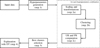 |
Fig. 1 Pipeline for clustering the data and explaining the output, given a subset of attributes and a minimum PR. |
2.3 Pipeline
Our classifier comes with a number of hyperparameters (parameters specific to the algorithm, rather than to the data) that need to be tuned. In order to do that, we followed the pipeline outlined in Fig. 1. We explain its main steps below:
Generate hyperparameter combinations;
-
For each hyperparameter combination:
- (a)
Apply data pre-processing (scaling and transformations);
- (b)
Fit GMM on the ULXs observations with an unknown nature;
- (c)
Select an optimal probability threshold on the output of GMM on confirmed PULX observations to maximize the UR for the given PR threshold of 99% (cf. Sect. 2.2);
- (a)
Select the best hyperparameters (i.e. the ones maximising UR);
Extract a DT that explains the clustering output.
The following subsections describe the relevant steps in more detail.
2.3.1 Scaling and transformations
First, the data were transformed based on the first three hyperparameters summarised in Table 2, in the following order:
Logarithmic scale on the fluxes and LPEAK (if the hyperparameter use_log is true);
Scaling, with the algorithms implemented in sklearn3 (Pedregosa et al. 2011);
Principal component analysis (PCA), if the hyperparameter use_PCA is True, with eight components to create new sets of uncorrelated variables, as shown in Krone-Martins & Moitinho (2013).
The scaling consists of adjusting the range of the attributes so that they fall within a specific interval or follow a distribution. In this work, we use min-max scaling4, standard scaling5, quantile transform6, and power transform7. Only one scaling method was used at a time and consistently applied across all attributes, ensuring they had similar ranges or distributions. Without scaling, some features might have dominated others due to differences in scale. Overall, PCA is a technique used for dimensionality reduction and feature extraction. It transforms the original set of attributes into a new set of uncorrelated attributes (the principal components) that can capture most of the variance in the original dataset.
Scaling, transformation, and GMM hyperparameters along with their values.
2.3.2 Clustering
We used GMM on the scaled and transformed data to group observations with similar properties together, with the purpose of finding candidate PULXs similar to the known ones. GMM is a probabilistic approach that can represent subpopulations with distinct characteristics inside a bigger population. GMM is a soft clustering algorithm: it assigns to each data point the probability of belonging to each cluster, in contrast to other algorithms that assign cluster labels (e.g. k-means; MacQueen et al. 1967), and relies on a probabilistic framework (Reynolds et al. 2009).
GMM outputs the weighted sum of M Gaussian component densities (Reynolds 2009) as
![Mathematical equation: $p\left[ {x|\lambda } \right] = \mathop \sum \limits_{c = 1}^M {w_c}g\left( {x|{\mu _c},{\Sigma _c}} \right),$](/articles/aa/full_html/2025/09/aa53739-25/aa53739-25-eq8.png) (8)
(8)
where x ∈ ℝd is the input of the model, d is the number of input parameters, g(x|μc, Σc) is a Gaussian (i.e. a component) with mean vector μc ∈ ℝd and covariance matrix Σc ∈ ℝd×d, and wc is the weight associated with each component. λ = {wc,μc, Σc}, with c ∈ 1, …, M, is the collection of the GMM weights, mean vectors, and covariance matrices. The weights, wc, can be interpreted as the proportion of the data associated with each component c.
First, we used the BayesianGaussianMixture implementation of GMM8 with two components (one per cluster), where the covariance type (full, tied, diag, or spherical, see Table 2) is the only variable hyperparameter and the priors for λ are the default ones. GMM was fitted only on the observations that are not associated with known PULXs. Then, GMM output the probabilities of each observation (in the entire dataset) belonging to the two clusters. Since the sum of the two probabilities for each observation is 1, we used only the probability to belong to the PULX cluster, hereafter. The probability threshold set at step 2(c) guarantees a minimum PR and maximises UR. Step 3 outputs the best clustering among all hyperparameter choices, that is, the one with the highest UR among those selected at step 2.
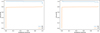 |
Fig. 2 UR and PR as a function of the probability threshold when considering both FPEAK and LPEAK (left panel) or only FPEAK (right panel), i.e. the two best cases reported in Table 3. |
2.3.3 Explainability
Binary DTs are non-parametric supervised learning algorithms used for classification and regression. They can model decisions by inferring rules from input features (Kingsford & Salzberg 2008). Such rules correspond to axis-aligned cuts in an n-dimensional space that separate values below and above a specific threshold for each input feature. We used DTs to approximate the best GMM outputs. To this end, GMM clusters are the target labels during the training of the DTs.
A DT is read from top to bottom. Each condition leads to two branches (when the condition is met, on the left, and when it is not met, on the right), so the leaves (i.e. the nodes without children) are not associated with conditions. Each node contains five pieces of information:
A condition used to determine the child nodes at the subsequent level;
gini, which is a decimal between 0 and 1 that represents the impurity of a node, where low values indicate that all the samples belong to the same cluster (noting that for two clusters, the gini value can go from 0 to 0.5, with the latter corresponding to the maximum impurity level).
samples, which indicates the number of samples before applying the condition;
value, which indicates the number of samples belonging to each of the clusters generated by GMM (in the format [ULX, PULX]) before applying the condition (i.e. considering only the region bounded by the preceding conditions in the tree);
class, which indicates the predicted cluster most of the observations in that node belong to.
DTs explainability depends on their leaves depth (i.e. the number of steps from the top node, or root, of the tree), as shown in Blanco-Justicia et al. (2020). In this work, we used shallow trees (up to a depth of 4) as they describe the obtained clusters well, are easier to interpret, and provide a set of measurable parameters with a physical interpretation. Table 1 lists and describes the parameters considered in this work.
Maximum UR achieved when considering or neglecting FPEAK or LPEAK and a minimum PR of 0.99.
3 Results
We ran the algorithm for four different cases: with both FPEAK and LPEAK, with only FPEAK, with only LPEAK, and without FPEAK and LPEAK. Table 3 shows the best UR for each case when PR is at least 0.99. Keeping FPEAK leads to the best results, while LPEAK has a negligible effect, independent of the presence of FPEAK. In this case, the best scaler is MinMaxScaler. Avoiding the logarithmic transformation yields better results, omitting PCA is preferable, and the best GMM covariance type is ‘full.’
In Fig. 2, we present the UR-PR plots as a function of the probability threshold for the two best cases listed in Table 3.
Whenever we keep FPEAK, the variations in PR are smaller as the probability threshold varies and the variations in UR are only observed when the probability threshold is 0 (i.e. all the observations are clustered together). The low variability and the high PR and UR values show that the pipeline can well separate the two clusters when keeping FPEAK and that the algorithm is robust to threshold variations. The curves are not monotonous because, by definition, PR is computed on the cluster containing most of the known PULXs and its value can never be lower than 0.5 by definition. When most of the known PULXs are below the probability threshold, the PULXs cluster (CP) is the one with low probabilities (intended as the probability of not observing a PULX).
From now on, we focus on the cases with FPEAK and without LPEAK and a minimum PR >0.99. All the parameters resulted in KS p-values <10–5, while the SI values are reported in Table 4. Bearing in mind that the SI values between 0 and +1 indicate that the clustering algorithm achieved a reliable assignment of the objects to their clusters, we found that both the KS p-values and SI values show that the data in the two clusters belong to significantly different distributions, even when considering each variable separately. Moreover, the average distance between points in the same cluster is smaller than the distance between points in different clusters, even when considering each variable separately.
In Fig. 3, we show the best DT, which explains GMM output for a minimum PR of 0.99. The DT uses six variables and shows that most of the new candidate PULXs are generally characterised by high fluxes (log(flux) > –12.387 in the 0.2–12 keV energy band). Among them, 37 observations (22 sources) were classified as PULXs have a high broadband flux, a low flux in the 4.5–12 keV energy band, and a high HRHard; however, gini >0 indicates that some observations not clustered with known PULXs also have the same characteristics. A smaller sample of candidate PULXs (43 observations of 10 sources) was also characterised by a high FPEAK (log(FPEAK) > –11.962). Finally, 22 observations (16 sources) with low fluxes, a low FPEAK, and flagged as variable were also classified as PULXs.
In Fig. 4, we give the distribution of the two clusters, CP and CU, using two examples of parameter combinations. The blue points indicate the observations belonging to CP (i.e. candidate and known PULXs), the red points those to CU, and the black circles indicate the observations of known PULXs (including those where pulsations are not detected). In the case of PR > 0.99, all the observations of known PULXs have been retrieved. The plots also show that the two clusters are not well-separated in two dimensions and highlight the need to consider multiple parameters. Comparing the plots and the DT shows that couples of parameters capture only a partial view of the DT. Figure 5 presents the distribution of two parameters: the broadband flux and HRHard. The cluster with candidate PULXs follows the same distribution as known PULXs, with a peak at high values of fluxes, while the HRHard distribution is similar for all three groups.
In Fig. 6, we present the distribution of the ULXs with respect to the probability determined by GMM. The orange bars refer to ULXs with no detected pulsations and the blue bars refer to PULXs. The red dashed line is the threshold τ (on the logarithm of the probability) corresponding to the confirmed PULX with the lowest probability. The orange bars above the τ are 85 new candidate PULXs (the complete list is reported in Table B.l), neglecting the PULX observation with the lowest probability, τ ≈ –0.04. As a result, 81 out of the 85 new candidate PULXs would still be identified as such. Considering all the 85 candidate PULXs, 52 sources have all the observations (276 in total) in the PULX cluster, and 33 have observations (206 in total) in both clusters (see Table C.l). Moreover, 549 sources do not have observations (1192 in total) in the PULX cluster. Overall, the candidate PULXs with all the observations in the PULX cluster are ≈8.6 times more than the confirmed PULXs, while only ≈5% of the sources (corresponding to ≈12% of the observations) are divided into multiple clusters.
In Fig. 7, we present the variation of the UR as a function of the source distance, for PR > 0.99, where for a given distance, all sources within that distance are considered. The UR is high and the variations in UR are small (≈ 10%) when keeping FPEAK. Finally, Fig. 8 shows the distribution of the candidate PULXs’ distances for PR > 0.99. Most candidates are found between 2 and 40 Mpc. Moreover, the distribution suggests that closer sources are slightly more likely to be selected as candidate PULXs.
 |
Fig. 3 DT that describes the output of GMM when keeping FPEAK and neglecting LPEAK, for PR = 0.99. Orange nodes correspond to a majority of ULXs, while blue nodes correspond to a majority of PULXs. |
Results for the SI for each variable in the case of FPEAK only.
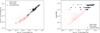 |
Fig. 4 2D representations of the two clusters considering two pairs of parameters. The blue dots are the observations belonging to the CP cluster, red dots are those belonging to the CU cluster, and black empty circles flag the known PULXs. |
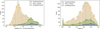 |
Fig. 5 Distributions of two relevant parameters when neglecting only LPEAK for the whole sample (orange), the confirmed PULXs (blue), and the candidate PULXs (green). |
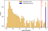 |
Fig. 6 Distribution of PULXs with respect to the GMM probability, in log-log scale. |
4 Discussion
The goal of this work is to highlight archival XMM-Newton observations of ULXs with similar characteristics to those of known PULXs in order to collect a sample of candidate PULXs based on the largest possible range of information for each of them. The novelty of this work is the use of ML methodologies, instead of more traditional techniques based on spectral and temporal analysis. In particular, we used GMM to cluster all data in two groups: one that collects the majority of known PULXs (CP) and one where the majority of ULXs have a compact object of unknown nature (CU). We used two parameters for the maximum flux and luminosity reached by the source (parameters FPEAK and LPEAK, Table 3). We found that only the former had an impact on our classifier.
In particular, for a PR > 0.99 (i.e. all known PULXs are correctly associated with the CP cluster) the best DT (see Fig. 3) can be reduced to just three main criteria to assign an observation to the PULX class: a) a broadband flux ≳4 × 10–13 erg cm–2 s–1; b) a maximum observed flux FPEAK ≳1 × 10–12 erg cm–2 s–1; and c) the presence of intra-observational fractional variability (VAR_FLAG ≥ 0.5). Based on this classification, the majority of observations in the CP cluster are those with the highest values of broadband fluxes (see also Fig. 5, left panel) and FPEAK. Inside the CP cluster, together with the known PULXs, there are 355 additional observations for a total of 85 unique sources (Table B.1) that constitute the candidate PULXs of this work.
Interestingly, parameters such as the hardness ratios or the fluxes in other energy bands do not seem to be decisive, as the DT shows that most of the instances are classified as PULXs independently of such parameters (Fig. 3). These parameters contribute to further refining the cluster membership without being discriminant. As a matter of fact, while the majority of instances assigned to the PULX cluster are sources caught in a hard state, some of them have softer spectra and are still classified as candidate PULXs, including those of known PULXs. In particular, this is true for the only observation of M51 ULX-7 at the minimum of the super-orbital period, classified as candidate PULX (Obsld.0830191401, with a flux of 2 × 10–14erg cm–2 s–1, where no pulsations were detected due to poor statistics; Rodríguez Castillo et al. 2020). A similar result holds for the observation of NGC 5907 ULX-1 when the source was at ~3×l0–14erg cm–2 s–1 and likely transitioning to a propeller regime (Obsld. 0824320501; Fürst et al. 2023). This is likely due to the parameter FPEAK imparting to the ML algorithm that the source is related to another observation with a higher flux. To check this hypothesis, we kept the Gaussian distributions fitted on the whole sample of ULXs (without the known PULXs) using GMM and the threshold determined on the original data. Then, we replaced the FPEAK values of the observations of known PULXs with the corresponding fluxes and computed the probabilities associated with the modified observations (this procedure does not modify the two initial Gaussians, but only affects where the points, corresponding to known PULXs, are positioned within the Gaussians). As a result, 13 observations of known PULXs (~ 14%) are not correctly classified in the PULX cluster, as their fluxes are particularly low. Of them, 12 observations (including Obsld.0830191401 of M51 ULX-7) do not show pulsations and only one (Obsld.0804090401) does; this observation corresponds to the observation of NGC 5907 ULX-1 with the lowest flux, where the spin signal is seen (Fürst et al. 2023). This finding suggests that the parameter FPEAK is important for a correct classification of low-flux observations, emphasising the need for multiple observations of ULXs, but it is not crucial, as most of the PULX observations are retrieved even without using FPEAK at testing time. Moreover, there are candidate PULXs with a low FPEAK (≈10–14 erg cm–2 s–1) and other ULXs with a high FPEAK (≈10–12 erg cm–2 s–1).
To further assess the robustness of our approach, we retain the fitted GMM and analyse the impact of removing either a single known PULX observation or all observations associated with a given PULX on the PR. Since GMM is fitted only on the sources with unknown nature, removing PULX observations affects only the threshold selection:
Removing a single observation: this affects the PR only when the lowest-probability observation is neglected. The average PR is computed by removing each observation (one at a time), recomputing the PR for the entire dataset after each removal, and then averaging these values. The resulting average PR is ≈99%;
Removing a source: we remove one source at a time, recompute the PR for the entire dataset after each removal, and then compute the average across all individual observations. The resulting average PR is ≈98%. Computing the average across sources, instead of observations, leads to a PR of ≈97%.
This result shows that the pipeline would retrieve observations that were not initially included in the dataset. The effectiveness in retrieving PULX observations, even when neglecting all the other observations of the same source, also shows that the pipeline does not rely only on source information such as FPEAK.
Concerning the distance of the sources (see Fig. 7), including sources within ~30Mpc (~60Mpc when considering both FPEAK and LPEAK) marginally influences the performances of the algorithm, with values of UR slightly smaller (keeping PR > 0.99), suggesting that a reduced number of sources is not sufficient to achieve the best configuration. At the same time, the greater the distance, the higher the chance of contamination of misclassified sources. This seems to have little to no effect on the output, as UR is approximately constant at distances ≳100Mpc (for the best case of PR > 0.99 and with only FPEAK). Understanding whether the plateauing of the UR metrics is due to the presence of contaminants would require knowledge of their ratio over the total sample and this is beyond the goal of this paper (see also below). Alternatively, the number of sources at distances ≳100Mpc might be too small to influence the metrics significantly. Regardless, we emphasise that this does not modify the main findings of the work since the greatest part of the new PULXs is within 25 Mpc.
Finally, a by-product of this work is the possibility of verifying the hypothesis that QPOs observed in ULXs can be used to mark the presence of an accreting NS (Imbrogno et al. 2024, Imbrogno et al., in prep.). We found that 19 observations out of 22 where QPOs have been reported in the literature (8 sources in total) are included in the sample of the 85 new candidate PULXs listed in CP (the remaining three observations are of M51 ULX-7). Although this finding is far from being conclusive, it is informative that known PULXs and ULXs with unknown accretors displaying QPOs share some similarity in the multidimensional phase space studied by the ML algorithm.
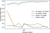 |
Fig. 7 UR as a function of the source distances, for different combinations of FPEAK and LPEAK and assuming a PR of 0.99. |
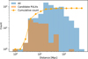 |
Fig. 8 Distribution of the candidate PULXs (orange) and of the whole observations (cyan) as a function of distance and the cumulative count of candidate PULXs. Most of them have distances ranging between 2 and 20 Mpc. The candidate PULXs are obtained for a minimum PR > 0.99. |
4.1 Biases and caveats
As for all ML algorithms, the goodness of the results is limited by the number and the quality of available observational data. This naturally introduces biases. First and foremost, not all sources have been observed the same number of times. In general, ULXs hosted in the galaxies with astrophysical objects of great interest to the community, including PULXs, have a higher number of observations (e.g. NGC 1313 X-1 and X-2 have all been observed more than 30 times). On the contrary, faint ULXs typically have a smaller number of observations, with the risk of missing out on potential high-flux phases. In fact, all candidate PULXs have the highest FPEAK values in the dataset (noting that FPEAK is equal to the flux of the observation if a source has been observed only once). This highlights the necessity to observe the sources multiple times in order to catch them in different luminosity states, so that we can determine the true FPEAK and correctly classify them as candidate PULXs or not. In particular, considering that pulsations have been detected in 31 out of 95 observations of known PULXs, assuming the same distribution for both known and unknown PULXs, we can infer that a ULX needs to be observed at least three times to have good chances (≈70%) to detect pulsations.
As mentioned above, another issue is the presence of contaminants, mostly foreground and background sources (e.g. AGNs), identified as point-like X-ray sources and associated with the wrong host galaxy. It is hard to obtain a precise estimate of the number of contaminants in the sample, but it has been noted that it grows as a function of distance, from a rate of ≲2% for nearby galaxies up to 70% for a pure HLX sample (see Tranin et al. 2024, and ref. therein). Considering that these distant contaminants usually display low fluxes, it can be reasonably excluded that they fall among the candidate PULXs found in this work; hence, the sample of candidates can be considered reasonably pure.
Lastly, several caveats in this work need to be borne in mind. First, all instances used for the clustering are directly taken from either the 4XMM-DR13 or the W22 catalogues. In particular, the values of the fluxes in the different energy bands are taken from the 4XMM catalogue, where they are derived by fitting all the spectra with the same absorbed power-law model, with fixed equivalent hydrogen column and photon index values (nH = 3 × 10²⁰ atoms cm–2, Γ = 1.7; Webb et al. 2020). However, this is not the best model for ULXs spectra, which are better fitted with a double-component model (such as multi-temperature discs or advection-dominated discs, see, e.g. Gúrpide et al. 2021) and, in some cases, with a high-energy cut-off (e.g. Walton et al. 2018). Hence, the fluxes used in this work are to be considered as an approximation of the actual source fluxes. Additionally, these fluxes are not corrected for interstellar or local absorptions and, hence, their temporal evolution does not accurately represent the intrinsic behaviour of the sources. Moreover, due to the use of a power-law model, the fluxes in different energy bands are not exactly independent instances. Nonetheless, all the parameters have undergone a PCA investigation (cf. Sect. 2.3.1), where eight components have been selected for the clustering algorithm. We stress that only some of the available information has been passed to the ML algorithm. In particular, all the fields containing the statistical uncertainties of the fluxes are not taken into account; therefore, considering each value as a ‘perfect’ measurement. This assumption likely introduces some unknown level of bias that cannot be addressed by the used ML algorithm.
The main limitation of many clustering algorithms is that the number of clusters needs to be specified in advance (Acquaviva 2023): in our approach, we considered only two clusters, representative of two classes of BH- and NS-ULXs. An alternative approach would be to consider the number of clusters NC as a free parameter, build a cluster scheme for different values of NC, and choose the one providing the best result (in terms of cost function). While powerful, this approach is more reliable with a larger number of observations than those currently available and would, in any case, still leave doubts regarding the physical interpretation of a greater number of clusters.
4.2 Candidate PULXs
While a detailed study of the candidate PULXs is beyond the aim of the present project and will be addressed in future works, we highlight the properties of some of them. In the PULX cluster, there are 355 observations of sources not previously identified as PULXs, for a total of 85 candidates (Tables B.1 and C.1). All the candidates occupy the upper right corner of the plots of Fig. 4. Hereafter, we briefly discuss the most promising ones.
The observations with the highest flux belong to M31 ULX-1, in the Andromeda Galaxy. The source reached its peak flux in 2009 (2 × 10–11 erg cm–2 s–1, corresponding to 1.3 × 1039 erg s–1 at a bona fide distance of 766 kpc), then slowly decayed. It was last detected by XMM-Newton in 2014. It has been interpreted as a stellar-mass BH in a low-mass X-ray binary temporarily undergoing (nearly) super-Eddington accretion (Middleton et al. 2012; Kaur et al. 2012).
A few other candidates have already been proposed as NS-ULXs. In particular, Quintin et al. (2021) already detected a pulsation from NGC 7793 ULX-4 during its only outburst at super-Eddington luminosity. Because the detection of the spin signal was only marginally significant (3.4σ, cf. Sect. 2.1), we excluded it from the sample of known PULXs used in this work. The clustering algorithm recovered it among the candidate PULXs, strengthening its nature as NS-ULX. Other good candidates include NGC 4559 X7, where a candidate pulsation with a significance of 3.5σ was recently found (Pintore et al. 2025); M81 X-6, suggested to host a weakly magnetised NS based on its spectral evolution (Amato et al. 2023); and IC 342 X-1 and NGC 925 ULX-1, previously identified as candidate PULXs because of their hardness ratios similar to that of known PULXs (Pintore et al. 2017, 2018).
The ML algorithm classifies as candidate PULXs also a few sources interpreted in the literature as BH-ULXs, such as Holmberg II X-1 (Barra et al. 2024), NGC 5240 X-1, NGC 5408 X-1 (e.g. Gúrpide et al. 2021), and NGC 7793 P9 (Hu et al. 2018). Other sources that do not offer sufficient spectral or temporal indications on the nature of their compact objects are also classified as candidate PULXs, such as NGC 1313 X-1 (e.g. Walton et al. 2020), IC 342 X-2, and NGC 5240 X-1. This strengthens the notion that traditional spectral or temporal analyses alone might not be able to uncover all the aspects of the ULX phenomenology.
We further note that for some sources, not all observations are assigned to the same cluster (see Table C.1). This is, for example, the case of M51 ULX-8, which has only one XMM-Newton observation (Obs ID.0677980801), out of 11, associated with the PULX cluster, likely due to the high flux and, correspondingly, high statistics of the given datasets. All the other XMM-Newton observations of this source resulted in low z-scores, preventing them from being associated with the same PULX cluster.
Finally, we carried out a preliminary timing analysis on the candidates by using the HENaccelsearch within the HENDRICS/Stingray software packages (Bachetti 2018; Huppenkothen et al. 2019; Bachetti et al. 2024), which accounts only for a first period derivative. We searched for pulsations from 0.1 Hz to the Nyquist frequency. The search gave negative results. More detailed timing analyses with both the traditional and AI evolutionary algorithms are needed in order to exhaustively study the new candidates (as done in Sacchi et al. 2024).
5 Conclusions and future perspectives
This work presents the results of the application of an unsuper-vised clustering pipeline to a database of ULX observations to identify new candidate PULXs relying upon all the available spectral and timing properties that are often neglected in standard analysis. We show that GMM determines, for each observation, the probability of belonging to the cluster containing the confirmed PULXs. Our pipeline assigns high probabilities to the observations of confirmed PULXs when the parameter FPEAK is taken into account. For this reason, the clustering effectively isolates candidate PULXs for a wide range of probability thresholds. In this case, retrieving at least 99% of the confirmed PULXs leads to 85 new candidate PULXs from 355 observations.
Future improvements of this work will focus on performing systematic fits of all ULX spectra with more appropriate models (cf. Sect. 4.1), allowing for better flux estimates in the different energy bands. The algorithm will be rerun on the updated database to obtain more robust results. Moreover, more reliable fluxes will lead to more precise luminosity estimates, so that the luminosities can also be employed as cluster parameters to better investigate the dependency of the results on the distance. The uncertainties on the best-fit parameters will also be taken into account (e.g. with bootstrapping) to increase the reliability of the results.
Another issue concerns the choice of the luminosity threshold of 1039 erg s–1 to select potential PULXs, as the mere existence of X-ray pulsars with luminosities in the ≈ 1034 – few 1038 erg s–1 range clearly casts doubts on its validity. Hence, an improvement on the present work will include observations of X-ray sources in the 2×1038–1039 erg s–1 range, which are potential X-ray pulsars in the super-Eddington regime. The inclusion of less luminous X-ray binaries can also contribute to the discussion of ULXs being an extension of the high-mass X-ray binary and PULXs of the X-ray pulsar populations. The proposed pipeline is part of a ‘living’ project and will be applied to new ULX observations when they are undertaken. For this purpose, we foresee the adoption of continual learning principles (Wang et al. 2024).
Acknowledgements
The database used in this research has been derived from the ULX catalogue of Walton et al. (2022) and the 4XMM-DR13 Webb et al. (2020), and it is available upon request. This study also uses observations obtained with XMM-Newton, a European Space Agency (ESA) science mission with instruments and contributions directly funded by ESA Member States and National Aeronautics and Space Administration (NASA). NOPV acknowledges support from INAF and CINECA for granting 125 000 core hours on the Leonardo supercomputer to carry out the project “Finding Pulsations with Evolutionary Algorithms”. MI is supported by the AASS Ph.D. joint research programme between the University of Rome “Sapienza” and the University of Rome “Tor Vergata”, with the collaboration of the National Institute of Astrophysics (INAF). RA and GLI acknowledge financial support from INAF through the grant “INAF-Astronomy Fellowships in Italy 2022 – (GOG)”. GLI also acknowledges support from PRIN MUR SEAWIND (2022Y2T94C), which was funded by NextGener-ationEU and INAF Grant BLOSSOM. KK is supported by a fellowship program at the Institute of Space Sciences (ICE-CSIC) funded by the program Unidad de Excelencia Maria de Maeztu CEX2020-001058-M.
References
- Acquaviva, V. 2023, Machine Learning for Physics and Astronomy [Google Scholar]
- Agrawal, V. K., & Nandi, A. 2015, MNRAS, 446, 3926 [NASA ADS] [CrossRef] [Google Scholar]
- Alashwal, H., El Halaby, M., Crouse, J. J., Abdalla, A., & Moustafa, A. A. 2019, Front. Computat. Neurosci., 13 [Google Scholar]
- Amato, R., Gúrpide, A., Webb, N. A., Godet, O., & Middleton, M. J. 2023, A&A, 669, A130 [NASA ADS] [CrossRef] [EDP Sciences] [Google Scholar]
- Assent, I. 2012, WIREs Data Mining Knowledge Discov., 2, 340 [Google Scholar]
- Atapin, K., Fabrika, S., & Caballero-García, M. D. 2019, MNRAS, 486, 2766 [NASA ADS] [CrossRef] [Google Scholar]
- Atapin, K., Vinokurov, A., Sarkisyan, A., et al. 2024, MNRAS, 527, 10185 [Google Scholar]
- Bachetti, M. 2018, HENDRICS: High ENergy Data Reduction Interface from the Command Shell, Astrophysics Source Code Library [record ascl:1805.019] [Google Scholar]
- Bachetti, M., Harrison, F. A., Walton, D. J., et al. 2014, Nature, 514, 202 [NASA ADS] [CrossRef] [Google Scholar]
- Bachetti, M., Huppenkothen, D., Stevens, A., et al. 2024, J. Open Source Softw., 9, 7389 [Google Scholar]
- Barra, F., Pinto, C., Middleton, M., et al. 2024, A&A, 682, A94 [NASA ADS] [CrossRef] [EDP Sciences] [Google Scholar]
- Belfiore, A., Salvaterra, R., Sidoli, L., et al. 2024, ApJ, 965, 78 [NASA ADS] [CrossRef] [Google Scholar]
- Blanco-Justicia, A., Domingo-Ferrer, J., Martínez, S., & Sánchez, D. 2020, Knowledge-Based Syst., 194, 105532 [Google Scholar]
- Brightman, M., Harrison, F. A., Fürst, F., et al. 2018, Nat. Astron., 2, 312 [CrossRef] [Google Scholar]
- Brightman, M., Walton, D. J., Xu, Y., et al. 2020, ApJ, 889, 71 [Google Scholar]
- Carpano, S., Haberl, F., Maitra, C., & Vasilopoulos, G. 2018, MNRAS, 476, L45 [NASA ADS] [CrossRef] [Google Scholar]
- Colbert, E. J. M., & Mushotzky, R. F. 1999, ApJ, 519, 89 [NASA ADS] [CrossRef] [Google Scholar]
- Colbert, E. J. M., Heckman, T. M., Ptak, A. F., Strickland, D. K., & Weaver, K. A. 2004, ApJ, 602, 231 [NASA ADS] [CrossRef] [Google Scholar]
- de Mijolla, D., Frye, C., Kunesch, M., Mansir, J., & Feige, I. 2020, arXiv e-prints [arXiv:2010.07384] [Google Scholar]
- Deng, Y., Tang, F., Dong, W., et al. 2019, Multimedia Tools Appl., 78, 19305 [Google Scholar]
- Dewangan, G. C., Griffiths, R. E., Choudhury, M., Miyaji, T., & Schurch, N. J. 2005, ApJ, 635, 198 [NASA ADS] [CrossRef] [Google Scholar]
- Evans, I. N., Primini, F. A., Miller, J. B., et al. 2020a, in American Astronomical Society Meeting Abstracts, 235, 154.05 [NASA ADS] [Google Scholar]
- Evans, P. A., Page, K. L., Osborne, J. P., et al. 2020b, ApJS, 247, 54 [Google Scholar]
- Fabbiano, G. 1989, ARA&A, 27, 87 [NASA ADS] [CrossRef] [Google Scholar]
- Fabrika, S. N., Atapin, K. E., Vinokurov, A. S., & Sholukhova, O. N. 2021, Astrophys. Bull., 76, 6 [NASA ADS] [CrossRef] [Google Scholar]
- Fürst, F., Walton, D. J., Harrison, F. A., et al. 2016, ApJ, 831, L14 [Google Scholar]
- Fürst, F., Walton, D. J., Heida, M., et al. 2021, A&A, 651, A75 [NASA ADS] [CrossRef] [EDP Sciences] [Google Scholar]
- Fürst, F., Walton, D. J., Israel, G. L., et al. 2023, A&A, 672, A140 [NASA ADS] [CrossRef] [EDP Sciences] [Google Scholar]
- Gladstone, J. C., Roberts, T. P., & Done, C. 2009, MNRAS, 397, 1836 [NASA ADS] [CrossRef] [Google Scholar]
- Gúrpide, A., Godet, O., Koliopanos, F., Webb, N., & Olive, J. F. 2021, A&A, 649, A104 [NASA ADS] [CrossRef] [EDP Sciences] [Google Scholar]
- Heil, L. M., Vaughan, S., & Roberts, T. P. 2009, MNRAS, 397, 1061 [CrossRef] [Google Scholar]
- Hu, C.-P., Kong, A. K. H., Ng, C. Y., & Li, K. L. 2018, ApJ, 864, 64 [Google Scholar]
- Huppenkothen, D., Bachetti, M., Stevens, A. L., et al. 2019, ApJ, 881, 39 [Google Scholar]
- Imbrogno, M., Motta, S. E., Amato, R., et al. 2024, A&A, 689, A284 [NASA ADS] [CrossRef] [EDP Sciences] [Google Scholar]
- ISO 2017, Standards by ISO/IEC JTC 1/SC 42 – Artificial Intelligence [Google Scholar]
- Israel, G. L., Belfiore, A., Stella, L., et al. 2017a, Science, 355, 817 [NASA ADS] [CrossRef] [Google Scholar]
- Israel, G. L., Papitto, A., Esposito, P., et al. 2017b, MNRAS, 466, L48 [NASA ADS] [CrossRef] [Google Scholar]
- Jain, A. K., & Dubes, R. C. 1988, Algorithms for Clustering Data (Prentice-Hall, Inc.) [Google Scholar]
- Kaaret, P., Feng, H., & Roberts, T. P. 2017, ARA&A, 55, 303 [Google Scholar]
- Kalogera, V., & Baym, G. 1996, ApJ, 470, L61 [NASA ADS] [CrossRef] [Google Scholar]
- Kaur, A., Henze, M., Haberl, F., et al. 2012, A&A, 538, A49 [NASA ADS] [CrossRef] [EDP Sciences] [Google Scholar]
- Kennea, J. A., Lien, A. Y., Krimm, H. A., Cenko, S. B., & Siegel, M. H. 2017, Astronomer’s Telegram, 10809, 1 [Google Scholar]
- King, A. R., Davies, M. B., Ward, M. J., Fabbiano, G., & Elvis, M. 2001, ApJ, 552, L109 [NASA ADS] [CrossRef] [Google Scholar]
- King, A., Lasota, J.-P., & Middleton, M. 2023, New A Rev., 96, 101672 [NASA ADS] [CrossRef] [Google Scholar]
- Kingsford, C., & Salzberg, S. L. 2008, Nat. Biotechnol., 26, 1011 [Google Scholar]
- Kirch, W., ed. 2008, Encyclopedia of Public Health (Springer Netherlands), 1484 [Google Scholar]
- Kovlakas, K., Zezas, A., Andrews, J. J., et al. 2020, MNRAS, 498, 4790 [Google Scholar]
- Krone-Martins, A., & Moitinho, A. 2013, A&A, 561, A57 [Google Scholar]
- MacQueen, J., et al. 1967, Some methods for classification and analysis of multivariate observations [Google Scholar]
- Majumder, S., Das, S., Agrawal, V. K., & Nandi, A. 2023, MNRAS, 526, 2086 [Google Scholar]
- Makarov, D., Prugniel, P., Terekhova, N., Courtois, H., & Vauglin, I. 2014, A&A, 570, A13 [NASA ADS] [CrossRef] [EDP Sciences] [Google Scholar]
- Massey, F. J. 1951, J. Am. Statist. Assoc., 46, 68 [CrossRef] [Google Scholar]
- Michaud, P. 1997, Future Gener. Comput. Syst., 13, 135 [Google Scholar]
- Middleton, M. J., Sutton, A. D., Roberts, T. P., Jackson, F. E., & Done, C. 2012, MNRAS, 420, 2969 [NASA ADS] [CrossRef] [Google Scholar]
- Mineo, S., Rappaport, S., Steinhorn, B., et al. 2013, ApJ, 771, 133 [Google Scholar]
- Pasham, D. R., Cenko, S. B., Zoghbi, A., et al. 2015, ApJ, 811, L11 [NASA ADS] [CrossRef] [Google Scholar]
- Pedregosa, F., Varoquaux, G., Gramfort, A., et al. 2011, J. Mach. Learn. Res., 12, 2825 [Google Scholar]
- Pinciroli Vago, N. O., & Fraternali, P. 2023, Neural Comput. Appl., 35, 19253 [Google Scholar]
- Pinto, C., & Walton, D. J. 2023, arXiv e-prints, [arXiv:2302.00006] [Google Scholar]
- Pinto, C., Walton, D. J., Kara, E., et al. 2020, MNRAS, 492, 4646 [Google Scholar]
- Pinto, C., Soria, R., Walton, D. J., et al. 2021, MNRAS, 505, 5058 [NASA ADS] [CrossRef] [Google Scholar]
- Pintore, F., Zampieri, L., Stella, L., et al. 2017, ApJ, 836, 113 [Google Scholar]
- Pintore, F., Zampieri, L., Mereghetti, S., et al. 2018, MNRAS, 479, 4271 [Google Scholar]
- Pintore, F., Pinto, C., Rodriguez-Castillo, G., et al. 2025, A&A, 695, A238 [NASA ADS] [CrossRef] [EDP Sciences] [Google Scholar]
- Poutanen, J., Lipunova, G., Fabrika, S., Butkevich, A. G., & Abolmasov, P. 2007, MNRAS, 377, 1187 [NASA ADS] [CrossRef] [Google Scholar]
- Pérez-Díaz, V. S., Martínez-Galarza, J. R., Caicedo, A., & D’Abrusco, R. 2024, MNRAS, 528, 4852 [CrossRef] [Google Scholar]
- Quintin, E., Webb, N. A., Gúrpide, A., Bachetti, M., & Fürst, F. 2021, MNRAS, 503, 5485 [NASA ADS] [CrossRef] [Google Scholar]
- Ransom, S. M., Eikenberry, S. S., & Middleditch, J. 2002, AJ, 124, 1788 [Google Scholar]
- Rao, F., Feng, H., & Kaaret, P. 2010, ApJ, 722, 620 [Google Scholar]
- Reynolds, D. 2009, Gaussian Mixture Models (Springer US), 659 [Google Scholar]
- Reynolds, D. A., et al. 2009, Encyclop. Biometrics, 741 [Google Scholar]
- Rodríguez Castillo, G. A., Israel, G. L., Belfiore, A., et al. 2020, ApJ, 895, 60 [Google Scholar]
- Rousseeuw, P. J. 1987, J. Computat. Appl. Math., 20, 53 [CrossRef] [Google Scholar]
- Sacchi, A., Imbrogno, M., Motta, S. E., et al. 2024, A&A, 689, A217 [NASA ADS] [CrossRef] [EDP Sciences] [Google Scholar]
- Sathyaprakash, R., Roberts, T. P., Walton, D. J., et al. 2019, MNRAS, 488, L35 [NASA ADS] [CrossRef] [Google Scholar]
- Sathyaprakash, R., Roberts, T. P., Grisé, F., et al. 2022, MNRAS, 511, 5346 [NASA ADS] [CrossRef] [Google Scholar]
- Sen, S., Agarwal, S., Chakraborty, P., & Singh, K. P. 2022, Exp. Astron., 53, 1 [NASA ADS] [CrossRef] [Google Scholar]
- Slijepcevic, I. V., Scaife, A. M. M., Walmsley, M., et al. 2022, MNRAS, 514, 2599 [NASA ADS] [CrossRef] [Google Scholar]
- Stoitsas, K., Bahulikar, S., de Munter, L., et al. 2022, Sci. Rep., 12, 16990 [Google Scholar]
- Strohmayer, T. E., & Mushotzky, R. F. 2009, ApJ, 703, 1386 [NASA ADS] [CrossRef] [Google Scholar]
- Strohmayer, T. E., & Markwardt, C. B. 2011, Astronomer’s Telegram, 3121, 1 [Google Scholar]
- Strohmayer, T. E., Mushotzky, R. F., Winter, L., et al. 2007, ApJ, 660, 580 [NASA ADS] [CrossRef] [Google Scholar]
- Strüder, L., Briel, U., Dennerl, K., et al. 2001, A&A, 365, L18 [Google Scholar]
- Sutton, A. D., Roberts, T. P., & Middleton, M. J. 2013, MNRAS, 435, 1758 [NASA ADS] [CrossRef] [Google Scholar]
- Townsend, L. J., Kennea, J. A., Coe, M. J., et al. 2017, MNRAS, 471, 3878 [NASA ADS] [CrossRef] [Google Scholar]
- Tranin, H., Webb, N., Godet, O., & Quintin, E. 2024, A&A, 681, A16 [NASA ADS] [CrossRef] [EDP Sciences] [Google Scholar]
- Tsygankov, S. S., Doroshenko, V., Lutovinov, A. A., Mushtukov, A. A., & Poutanen, J. 2017, A&A, 605, A39 [NASA ADS] [CrossRef] [EDP Sciences] [Google Scholar]
- Vasilopoulos, G., Ray, P. S., Gendreau, K. C., et al. 2020, MNRAS, 494, 5350 [NASA ADS] [CrossRef] [Google Scholar]
- Virtanen, P., Gommers, R., Oliphant, T. E., et al. 2020, Nat. Methods, 17, 261 [Google Scholar]
- Walton, D. J., Fürst, F., Heida, M., et al. 2018, ApJ, 856, 128 [NASA ADS] [CrossRef] [Google Scholar]
- Walton, D. J., Pinto, C., Nowak, M., et al. 2020, MNRAS, 494, 6012 [Google Scholar]
- Walton, D. J., Mackenzie, A. D. A., Gully, H., et al. 2022, MNRAS, 509, 1587 [Google Scholar]
- Wang, L., Zhang, X., Su, H., & Zhu, J. 2024, IEEE Trans. Pattern Anal. Mach. Intell., 46, 5362 [Google Scholar]
- Webb, N. A., Coriat, M., Traulsen, I., et al. 2020, A&A, 641, A136 [NASA ADS] [CrossRef] [EDP Sciences] [Google Scholar]
- Weng, S.-S., Ge, M.-Y., Zhao, H.-H., et al. 2017, ApJ, 843, 69 [Google Scholar]
- Wiktorowicz, G., Sobolewska, M., Lasota, J.-P., & Belczynski, K. 2017, ApJ, 846, 17 [NASA ADS] [CrossRef] [Google Scholar]
- Wilson-Hodge, C. A., Malacaria, C., Jenke, P. A., et al. 2018, ApJ, 863, 9 [Google Scholar]
- Zampieri, L., & Roberts, T. P. 2009, MNRAS, 400, 677 [NASA ADS] [CrossRef] [Google Scholar]
Appendix A Observations of known PULXs
Predicted z-scores for all the known PULXs in the dataset grouped by name.
Appendix B New candidate PULXs
Predicted z-scores for the 85 candidate PULXs, sorted by coordinates.
Appendix C Subdivision of candidate PULXs in clusters
Number of observations classified by the clustering algorithm as candidates (cluster CP) and non-candidates (cluster CU) for each source (excluding known PULXs) and the percentage of observations identified as candidates relative to the total number of observations per source.
M82 X-1 and X-2 are separated only by 5″, (see e.g. Brightman et al. 2020). XMM-Newton point spread function (PSF) sizes are 6.6″, 6.0″ and 4.5″ for EPIC-pn, MOS1 and MOS2, respectively (FWHM at 1.5 keV, https://xmm-tools.cosmos.esa.int/external/xmm_user_support/documentation/uhb/xmmpsf.html).
All Tables
Maximum UR achieved when considering or neglecting FPEAK or LPEAK and a minimum PR of 0.99.
Number of observations classified by the clustering algorithm as candidates (cluster CP) and non-candidates (cluster CU) for each source (excluding known PULXs) and the percentage of observations identified as candidates relative to the total number of observations per source.
All Figures
|
Fig. 1 Pipeline for clustering the data and explaining the output, given a subset of attributes and a minimum PR. |
| In the text | |
|
Fig. 2 UR and PR as a function of the probability threshold when considering both FPEAK and LPEAK (left panel) or only FPEAK (right panel), i.e. the two best cases reported in Table 3. |
| In the text | |
|
Fig. 3 DT that describes the output of GMM when keeping FPEAK and neglecting LPEAK, for PR = 0.99. Orange nodes correspond to a majority of ULXs, while blue nodes correspond to a majority of PULXs. |
| In the text | |
|
Fig. 4 2D representations of the two clusters considering two pairs of parameters. The blue dots are the observations belonging to the CP cluster, red dots are those belonging to the CU cluster, and black empty circles flag the known PULXs. |
| In the text | |
|
Fig. 5 Distributions of two relevant parameters when neglecting only LPEAK for the whole sample (orange), the confirmed PULXs (blue), and the candidate PULXs (green). |
| In the text | |
|
Fig. 6 Distribution of PULXs with respect to the GMM probability, in log-log scale. |
| In the text | |
|
Fig. 7 UR as a function of the source distances, for different combinations of FPEAK and LPEAK and assuming a PR of 0.99. |
| In the text | |
|
Fig. 8 Distribution of the candidate PULXs (orange) and of the whole observations (cyan) as a function of distance and the cumulative count of candidate PULXs. Most of them have distances ranging between 2 and 20 Mpc. The candidate PULXs are obtained for a minimum PR > 0.99. |
| In the text | |
Current usage metrics show cumulative count of Article Views (full-text article views including HTML views, PDF and ePub downloads, according to the available data) and Abstracts Views on Vision4Press platform.
Data correspond to usage on the plateform after 2015. The current usage metrics is available 48-96 hours after online publication and is updated daily on week days.
Initial download of the metrics may take a while.