| Issue |
A&A
Volume 701, September 2025
|
|
|---|---|---|
| Article Number | A209 | |
| Number of page(s) | 16 | |
| Section | Planets, planetary systems, and small bodies | |
| DOI | https://doi.org/10.1051/0004-6361/202553953 | |
| Published online | 16 September 2025 | |
Hybrid simulations of Mercury’s global dynamics and the interplanetary ions’ precipitation fluxes under different interplanetary conditions
1
Laboratoire de Physique des Plasmas (LPP), CNRS, Observatoire de Paris, Sorbonne Université, Université Paris-Saclay, École Polytechnique, Institut Polytechnique de Paris,
Palaiseau
91120,
France
2
Laboratoire Atmosphères, Milieux et Observations Spatiales (LATMOS), IPSL, CNRS, UVSQ-Université Paris-Saclay, Sorbonne Université, CNES,
Paris,
France
★ Corresponding author.
Received:
29
January
2025
Accepted:
11
July
2025
Abstract
Aims. We aim to quantify the impact of different interplanetary conditions met by Mercury along its orbit between its aphelion (~0.47 AU) and perihelion (~0.31 AU) on the Hermean environment, including the rate of solar-wind ion precipitation onto the surface.
Methods. We performed a set of 3D global hybrid simulations (kinetic ions and fluid electrons) with interplanetary conditions taken from recent statistics from observations on board the Parker Solar Probe and MESSENGER missions in such a way as to represent an average scenario at both the aphelion and perihelion positions, and in the cases of a slow (250 km/s) and fast (450 km/s) solar wind.
Results. The results are in general agreement with empirical models. However, we have found that the subsolar stand-off distances of magnetopause and bow shock, respectively, in the range of 1.0–1.4 RM and 1.3–2.0 RM, are relatively shorter than global statistical averages of, respectively, 1.45 and 1.96 RM. We also observe a local time (LT) asymmetry in the cusp’s location, with the northern cusp located in the post-noon sector centred around 13–14.3 LT and the southern cusp located in the pre-noon sector centred around 9–10.7 LT. Noticeably, the southern cusp region takes the shape of a parallelogram extended from southern middle latitudes in the pre-noon sector to equatorial latitudes in the post-noon sector. We suggest that these effects could result from the orientation of the interplanetary magnetic field along the Parker spiral, which is characterised by an almost radial orientation with a small duskward component.
Key words: plasmas / methods: numerical / planets and satellites: dynamical evolution and stability / planets and satellites: magnetic fields / planets and satellites: individual: Mercury
© The Authors 2025
 Open Access article, published by EDP Sciences, under the terms of the Creative Commons Attribution License (https://creativecommons.org/licenses/by/4.0), which permits unrestricted use, distribution, and reproduction in any medium, provided the original work is properly cited.
This article is published in open access under the Subscribe to Open model. This email address is being protected from spambots. You need JavaScript enabled to view it. to support open access publication.
1 Introduction
The precipitation of ions on the surface of Mercury plays a crucial role in the sputtering process at the origin of exospheric planetary neutrals (Leblanc & Johnson 2003, 2010; Milillo et al. 2005). In particular, the magnetospheric polarcusps represent a natural access to the surface for solar wind ions. For instance, ground-based observations revealed that the solar-wind ion precipitation through polar cusps is closely related to sodium emission (Mangano et al. 2015). The MErcury Surface, Space ENvironment, GEochemistry, and Ranging (MESSENGER) observations provided more insight into the role of solar wind ion precipitation in the production of different neutral species (Zurbuchen et al. 2011). In addition, a sodium emission may even be considered as a proxy for solar perturbations transit (Orsini et al. 2018).
The couplings between interplanetary and planetary media are recognised as the major players in governing the dynamics of Mercury’s environment. As characterised by the Mariner-10 mission and MESSENGER, Mercury features an intrinsically induced southward-directed, spin-aligned, dipole-like magnetic field much weaker than Earth ( ) and shifted ~484 km northwards (Anderson et al. 2011). Similarly to Earth, it develops a magnetosphere, yet smaller. Winslow et al. (2013) inferred that the average subsolar stand-off distances of the magnetopause and bow shock are, respectively, about 1.5 and 2 RM, which is about seven times smaller than for the Earth. The timescales are also reduced with a much faster Dungey cycle than the terrestrial one (order of seconds and minutes versus order of hours), showing high reconnection rates as to indicate that the magnetosphere is particularly sensitive to different interplanetary environments (Slavin et al. 2010; Imber & Slavin 2017).
Due to its eccentric orbit around the Sun, Mercury faces significantly different interplanetary conditions between its aphelion and perihelion positions at, respectively, ~0.31 AU and ~0.47 AU. For example, the interplanetary magnetic field (IMF) intensity and particle density can increase on average two or more times (James et al. 2017; Sun et al. 2022). In addition, fluctuations in the interplanetary medium can be very strong, and extreme solar events may substantially compress the magnetopause and the bow shock towards the surface, even causing the disappearance of the day-side magnetopause (Slavin et al. 2014, 2019; James et al. 2017; Winslow et al. 2017, 2020; Guo et al. 2023).
Computer simulations brought new insights into the complex dynamics of the magnetosphere of Mercury. For example, magnetohydrodynamic and fluid simulations revealed the importance of taking into account the induction effects of the presence of a conducting core electromagnetically coupled to the magneto-spheric plasma (Jia et al. 2015; Dong et al. 2019). A sufficiently dense exosphere of sodium leads to a shielding of the ambient electric field and contributes to an inflation of the magnetosphere, as demonstrated by Exner et al. (2020) with hybrid simulations. Furthermore, fully kinetic simulations showed that electrons contribute to the global dynamics by playing a crucial role in several small-scale physical processes, such as the thinning and enhancement of current sheets, as well as particles acceleration (Lapenta et al. 2022; Lavorenti et al. 2022). One of the most important effects on the global shape and dynamics of the magnetosphere of Mercury comes from the interplanetary magnetic field and the solar wind (e.g. Kallio & Janhunen 2003, 2004; Fatemi et al. 2020). In a comprehensive study involving 3D hybrid simulations of different conditions in the interplanetary medium, Fatemi et al. (2020) predicted the precipitation of high proton fluxes in the cusps of both hemispheres, centred around noon with latitudinal and longitudinal extents of 11° and 21° on average. In particular, they showed that this double-peak pattern is mainly controlled by the radial component of the IMF rather than its out-of-ecliptic component (Bz). They suggested that the entire surface of Mercury on the day side should be exposed to the solar wind when its dynamic pressure exceeds 70 nPa.
In addition to MESSENGER, the description of the inter-planetary medium in Mercury’s orbital zone also benefits from the observations of recent missions. From Parker Solar Probe observations, Sun et al. (2022) inferred an increase in plasma density, temperature, and interplanetary magnetic field of about three times between the aphelion and the perihelion positions. Although very variable, the IMF average orientation investigated from MESSENGER observations predominantly follows the Parker spiral in the ecliptic plane, which shows an almost radial configuration with a small angle in the 25° to 17° range between the aphelion and the perihelion (James et al. 2017). In the cusp regions, large IMF disturbances are preferably observed at perihelion and for negative north-south component of the magnetic field (He et al. 2017). Finally, crossings of the northern cusp were found statistically between 50°N–85°N in magnetic latitude, nearly centred in the same location but with a very variable extent over different orbits, and proton precipitation fluxes on the order of 1011 to 1013 m−2 s−1 (Raines et al. 2022).
In summary, a considerable amount of quantitative information has recently been accumulated from these in-depth statistical studies. However, some questions remain only partially or completely addressed. For example, the southern cusp is expected to occur at more equatorial latitudes than the northern cusps due to a weaker surface magnetic field. However, its dynamics, as well as the dependence of the precipitation fluxes on the interplanetary parameters, would require further studies. Strong orbit-to-orbit variations were observed on the local time (LT) and latitude of the cusp crossings and on the heliospheric distances, but they have not been investigated more deeply. Another important question concerns the sputtering efficiency of the Hermean surface when hit by solar wind particles, as one of the possible sources of the planetary exosphere. In the absence of detailed observations, this mechanism is commonly assumed to occur at energies of precipitating ions greater than one kiloelectronvolt (e.g. Lavorenti et al. 2023, and references therein). Better knowledge of both the location and the energy distribution of ion precipitation fluxes is of primary interest to improve the estimates of the sputtering effect.
In order to provide new insights to compare with future observations from the BepiColombo mission, we used 3D hybrid simulations to investigate the dynamics of the Mercury magnetic environment and the solar-wind proton precipitation. We considered the average interplanetary conditions inferred from the aforementioned recent statistical studies at the two extreme aphelion and perihelion positions along the orbit.
The paper is structured as follows. Sect. 2 introduces the numerical setup and the methodology used to obtain the results presented and described in Sect. 3. A discussion of the results and conclusions are given in Sects. 4 and 5.
2 Simulation setup
For the simulations, we adapted the 3D multi-species MPI-parallelised hybrid code LatHyS (Modolo et al. 2016), which was already successfully used to study the interaction of magnetic clouds with the terrestrial bow shock (Turc et al. 2015) and magnetosheath (Moissard et al. 2019), as well as the interaction of solar wind with the environments of the Earth (Cazzola et al. 2023), Mars (Modolo et al. 2016; Romanelli et al. 2018), Venus (Aizawa et al. 2022), and Mercury (Richer et al. 2012). Ions are treated in a kinetic fashion, whereas electrons are considered as a neutralizing background fluid with an adiabatic description.
We adopted the Mercury solar orbital (MSO) coordinates, with the origin at the centre of Mercury, the X-axis pointing towards the Sun, the positive Y-axis towards dusk, and the Z-axis towards the north. The radius of Mercury (RM) is ~2440 km. Its magnetosphere is self-consistently generated with a dipole characterised by a dipolar magnetic moment of  oriented along −Z and shifted northwards by 484 km (~0.198 RM), as found by Anderson et al. (2011). Unless specified otherwise, the magnetic equator refers to the plane parallel to the equatorial plane at Z = 484 km. The magnetic field inclination and planetary rotation have been neglected. The planet in the simulation acts as an inner boundary with purely absorbing properties: particles crossing this boundary are considered absorbed. Given the still uncertain insights into its structure, we have not considered any conductivity or resistivity modelling of the planetary interior nor for the surface. As well, the presence of an exosphere is not taken into account. These assumptions are discussed in Sect. 4.
The description of the interplanetary medium is based on the recent statistical review by Sun et al. (2022) as a function of the distance from the Sun (between 0.25 and 1 AU) from observations by the Parker Solar probe and WIND. In the work presented here, we used these results for Mercury’s orbital position at perihelion (~0.3 AU) and aphelion (~0.47 AU), which are summarised in Table 1. Specifically, the average density in the solar wind is seen to decrease by a factor of ~2.5 from perihelion to aphelion (from about 100 cm−3 to 40 cm−3). The ion’s temperature also decreases from 1.5 ⋅ 105 K to 3 ⋅ 104 K. The magnetic-field intensity decreases by a factor of three from 45 nT to 15 nT. The IMF direction was chosen following what was found in James et al. (2017) and He et al. (2017), where they showed that its variable orientation is predominantly seen in the ecliptic plane with an average direction in agreement with the Parker spiral angle. Hence, the chosen IMF directions feature an angle of 17° to 25° from the Mercury-Sun line for the perihelion and aphelion scenarios, respectively. In particular, the IMF component was chosen to be directed planetwards and duskwards. The out-of-ecliptic-plane Bz component is neglected in order to avoid processes that might favour the onset of magnetic reconnection.
Sun et al. (2022) found a constant velocity of the solar wind in the orbital range of Mercury of the order of 330 km/s, with small variations in the 250–450 km/s range. We decided to consider these two limits as representative cases of slow and fast solar wind. Therefore, in this work we considered four representative scenarios for the interplanetary conditions: the two scenarios at aphelion and perihelion, each of them including two sub-scenarios at different solar wind velocities to take into account the effects of slow solar wind (SSW) at 250 km/s and fast solar wind (FSW) at 450 km/s. Table 1 also highlights that these four scenarios cover a wide range of interplanetary conditions in terms of solar-wind dynamic pressure (from about 4 to 35 nPa) and Alfvén Mach number (from 2 to 9).
The simulation box is based on a 3D cartesian grid with open boundary conditions on the two opposite input and output planes perpendicular to the X-axis and periodic boundary conditions on the other edges. The solar wind enters the system homogeneously from the input boundary and uniformly flows towards the output edge. The box size is about (12 × 21.2 × 21.2) RM. Depending on the scenario, it features (810 × 1440 × 1440) di with a space resolution of ∆x = ∆y = ∆z = 3 di for the aphelion case, and (1280 × 2272 × 2272) di with a space resolution of ∆x = ∆y = ∆z = 4 di for the perihelion case (di being the ion skin depth of the pristine solar wind and read, respectively, di = 35.88 km and di = 22.69 km). The adopted time step is  for the aphelion case and
  for the perihelion case, where ωci is the ion cyclotron frequency reading
  and
and  , respectively. All values are normalised to the pristine solar wind conditions. Only protons and helium particles were considered in the simulations, in the proportion of 5% helium and 95% hydrogen.
At initialisation, solar-wind particles are loaded uniformly in the whole domain. In order to eliminate artificial effects due to trapped particles in the initial dipolar field, the magnetic dipole is allowed to progressively grow in intensity over the first cycles to smoothly achieve its nominal value and to self-consistently generate Mercury’s bow shock and magnetopause, until the steady state is achieved.
Interplanetary conditions adopted in this work.
3 Results
3.1 Global dynamics
The results for these four scenarios are displayed in Figs. 1, A.1, A.2, and A.3, which represent the distribution on the meridian plane (upper row), the magnetic equatorial plane (lower row) of the magnetic-field intensity (left panels), the current components Jz and Jy (top and bottom middle panels), and the density (right panels). In this illustration, the solar wind flows from the right to the left side. For the sake of visualisation, only a subset box is displayed for all plots. For each map, we superimpose the shape of the magnetopause and bow shock as predicted by the model proposed by Winslow et al. (2013) with dotted lines. Each scenario is analysed in more detail in the following sections.
3.1.1 Aphelion slow solar-wind scenario
The first scenario describes the situation with the weakest density (40 cm−3), the slowest solar-wind bulk velocity (250 km/s) and the weakest magnetic-field intensity (15 nT). The dynamic pressure is thus low (~4.2 nPa) and the Alfvén Mach number of the order of 5. Figure 1 shows that the magnetopause and bow shock are clearly identified by density and magnetic jumps and by enhanced current circulation. The subsolar stand-off distances are a particularly important parameter to characterise the penetration of solar fluxes towards the planetary surface. From the results, the magnetopause stand-off distance is found very close to the planet at about 1.39 RM, while that of bow shock is found at around 2.02 RM. As expected, the magnetosheath in between is compressed with enhanced values of the magnetic field (left panels) and density (right panels) compared to the pristine solar wind conditions.
A glaring feature is the magnetosheath asymmetry in the equatorial plane (bottom row), with a dawn side much more disturbed and thinner than the dusk side. The same does not appear in the meridian plane, which shows a very symmetric shape and a thicker magnetosheath. This is due to the orientation of the interplanetary magnetic field: given its 25° angle with the x-axis, the dawn side is the region where the interaction with the bow shock belongs to the quasi-parallel configuration. As such, a strong foreshock region forms, which is caused by the reflection of solar-wind particles by the bow-shock front and their subsequent interaction with the same incoming solar wind, generating a region of high turbulence and instabilities (e.g. Eastwood et al. 2005).
The superimposed dotted lines represent the average bow shock and magnetopause shapes from the model proposed in Winslow et al. (2012) based on a symmetric paraboloidal parametrisation underpinned by the magnitude of the dynamic pressure and the Alfvén Mach number. We can see that in this scenario the predicted and simulated global shapes and locations are consistent overall. The largest discrepancy is on the dawn side and may be due to the inability of a symmetric statistical model to capture asymmetric features, such as the foreshock region. The magnetopause and bow-shock equatorial stand-off distances also appear to be consistent (even though they are slightly shorter than those predicted by the empirical model of 1.74 and 2.2 RM, respectively). These small differences could be due to the fact that the simulated interplanetary conditions are outside the application domain of the statistical model, since a dynamic pressure of 4.2 nPa is outside its validity range (8.8–21.6 nPa); this is discussed in Sect. 4.
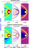 |
Fig. 1 Aphelion SSW scenario. Upper panels show a cross-section in the meridian plane (at Y = 0 km), while lower panels show a cross-section along the magnetic equatorial plane (at Z = 484 km). Each row shows the maps of the magnetic-field intensity, B, the current components (JZ in upper panel and JY in lower panel), and the particle density. The dotted black lines represent the predicted magnetopause and bow shock’s shapes based on the model proposed in Winslow et al. (2013). The Sun is ideally located on the right edge, and the solar wind flows from the right edge to left. |
3.1.2 Aphelion fast solar-wind scenario
With a higher solar-wind velocity (450 km/s), this scenario presents a higher dynamic pressure (~13.5 nPa) and a higher Alvénic Mach number (i.e. 8.6) than the previous case. Under these conditions, both the magnetopause and the bow shock contract towards the planetary surface, as shown in Fig. A.1. Their subsolar stand-off distances are now 1.07 and 1.47 RM, respectively.
The subsolar magnetosheath has become very thin, i.e. ~916 km, which is about three times the convective gyroradius (i.e. 313 km) defined as the ratio between the solar-wind velocity and the ion cyclotron frequency (e.g. Moses et al. 1988; Gedalin 2020). It has been found that a typical scale length up to three convective gyroradii in the bow shock downstream was necessary for particle thermalisation (Livesey et al. 1982; Scudder et al. 1984). In such a narrow subsolar magnetosheath, particles may not reach their thermal equilibrium before their interaction at high energy with the magnetopause.
Similarly to the previous case, the bow shock on the dawn side is affected by the presence of a foreshock region. Due to a higher solar-wind velocity and higher Alfvénic Mach number, the foreshock becomes even more intense, so the turbulence in the magnetosheath increases, causing strong fluctuations of the magnetic field, density, and currents (bottom row in Fig. A.1). The shape and location of both magnetopause and bow shock are in excellent agreement with their predictions from the model. Besides the foreshock region, which is not taken into account in the statistical model, the main difference concerns the subsolar region: the equatorial stand-off distances appear much closer to the planet than predicted by the model (the latter being about 1.46 and ~2 RM, respectively). The possible reasons of these discrepancies are discussed in Sect. 4.
3.1.3 Perihelion slow solar-wind scenario
Despite a larger solar-wind density (100 cm−3) but a lower velocity (250 km/s), this scenario features a dynamic pressure (10.45 nPa) comparable to the previous case of aphelion FSW (13.54 nPa). However, with a larger interplanetary magnetic field of 45 nT, the Alfvénic Mach number drops from 8.6 to 2.53. The outcome of this scenario is shown in Fig. A.2. With respect to those from the previous case (i.e. Fig. A.1), we observe that such a low Alfvén Mach number induces a bow-shock expansion to farther distances from the planet (1.86 RM versus 1.47 RM) and broader wings in both the meridian and magnetic equatorial planes. A low Alfvén Mach number also influences the intensity of the foreshock: it becomes difficult to observe the disturbances, which are still present, but not significantly affecting the dawn side or the bow shock boundary. Indeed, the currents flowing on the magnetopause and bow shock’s surface seem to be reinforced (see Jy in Fig. A.2). By comparing this scenario with the other similar case under SSW at the aphelion point in Fig. 1, we observe that the magnetopause and bow-shock stand-off distances are now shorter, i.e. 1.16 and 1.86 RM versus 1.39 and 2.02 RM, respectively. This difference seems to be driven by the large variation in the dynamic pressure, which is twice as high in this scenario as that shown in Fig. 1. Finally, a comparison with the statistical model reveals a global agreement, even though some discrepancies are still present. We note a shorter value of subsolar stand-off distances than that predicted by the model (i.e. 1.52 and 2.47 RM for the magnetopause and bow shock, respectively). The bow shock flaring also differs even more than expected because of the presence of a foreshock region. These discrepancies are probably due to the fact that an Alfvénic Mach number as low as 2.53 is outside the validity range of the model (i.e. 4.12 < MA < 8.11), and this is discussed in Sect. 4.
3.1.4 Perihelion fast solar-wind scenario
Compared to the previous case, an increase in solar-wind velocity from 250 to 450 km/s contributes to a significant increase in both the dynamic pressure, reaching a very high value (i.e. ~34 nPa) and, to a lesser extent, the Alfvén Mach number (i.e. from 2.53 to 4.56). Under these conditions, both the magnetopause and the bow shock strongly contract towards the planet, as shown in Fig. A.3. Their subsolar stand-off distances are now reduced to approximately 1 RM and 1 .32 RM, and the magnetopause is now pushed to the surface. As expected, an increase in the Mach number corresponds to an increase in the perturbation in both the foreshock region and the associated downstream magnetosheath (dawn side).
The statistical model of Winslow et al. (2013) has also been extrapolated for this case, even though such a high dynamic pressure far exceeds its application range (8.8–21.6 nPa), predicting a value of 1.11 RM and 3.07 RM, respectively. The boundaries’ shapes appear to be comparable, except for the dawn side, which also occurred for the other cases. However, the most significant feature of this scenario is the extreme contraction of the subsolar region towards the planet.
3.1.5 Summary of the global dynamics effects
In summary, we considered four scenarios describing the aphelion and perihelion positions embedded in both slow and fast solar winds. The results globally show a magnetopause with a cylindrical shape after 2 RM downtail and a bow-shock with a flaring decreasing with the Alfvénic Mach number, as expected.
In addition, we observed the overall formation of an asymmetric magnetosheath, with a dawn side much thinner and more turbulent than all other sides, which is common to all the scenarios. This is due to the orientation of the interplanetary magnetic field in the equatorial plane with a small angle with respect to the x-axis. This outcome is consistent with the simulations performed by Fatemi et al. (2020). On the dawn side, the interaction with the bow shock belongs to a quasi-parallel configuration, and the magnetosheath is expected to be thinner, based on the solar wind – magnetosphere coupling properties (e.g. Walsh et al. 2014). This type of interaction also creates a strong fore-shock region caused by the reflection of solar-wind particles from the bow-shock front and their subsequent interaction with the incoming solar wind, creating a region of high turbulence and instability (e.g. Eastwood et al. 2005). The latter contributes to a significant disruption of the bow-shock boundary in this side, possibly also affecting the clear identification of the subsolar stand-off distance.
The subsolar environment, in turn, appears to be strongly dependent on the interplanetary conditions. The subsolar standoff distances of the bow shock and magnetopause for the four scenarios are summarised in Table 2. When comparing the scenarios under the same solar-wind speed, as the planet moves from aphelion to perihelion, we can see that the stand-off distance decreases by 10–20% for the magnetopause and by 8–10% for the bow shock. In comparing the scenarios in the same orbital position, it is evident that a FSW (450 km/s) has a stronger effect in the aphelion position than a SSW (250 km/s); it reduces the magnetopause and bow-shock stand-off distances by between 20 and 30%. In the perihelion scenario, the FSW instead induces a limited magnetopause compression of ~13%, whereas the bow shock still undertakes a compression of ~30%.
Additionally, there may be cases where the thickness of the magnetosheath is reduced to less than three times the convective gyroradius (defined as the ratio of solar-wind velocity to ion cyclotron frequency (e.g. Moses et al. 1988; Gedalin 2020)), such as at aphelion under FSW. In this case, the energetic ions of the incoming solar wind cannot be fully thermalised in the magnetosheath and may impact the magnetosphere directly with high energy.
Finally, the simulated shape, position, and dynamics of the magnetopause and the bow shock are found to be globally consistent with the empirical model proposed by Winslow et al. (2012), even though it was extrapolated outside its validity domain for some cases. As expected, this symmetric paraboloidal model cannot describe asymmetric features such as the impact of the quasi-parallel configuration in the equatorial plane on the dawn side of the shock due to the quasi-radial IMF. In the case of the FSW at aphelion, both the solar-wind dynamic pressure and the Alfvén Mach-number are inside the model’s validity domain. The numerical and empirical models are then found in excellent agreement everywhere except in the subsolar region that is predicted to be closer to the planet. This difference is discussed in detail in Sect. 4.
Values of magnetopause and bow shock’s stand-off distances on magnetic equator from simulations.
3.2 Ion precipitation fluxes
3.2.1 Global maps
One of the consequences of the bow shock and magnetopause’s proximity to the planet is the number of solar wind particles that can precipitate directly to the surface. Their impact can represent a significant source of neutrals and ions, i.e. from sputtering mechanisms (e.g. Wurz & Lammer 2003). In this section, we focus on the location, rate, and extent of solar-wind ions precipitating on Mercury’s surface in the different scenarios considered. Similarly to Fatemi et al. (2020), we evaluated this rate as the number of particles crossing a nominal surface ideally set at a specific altitude close to the surface; here, 50 km. Only those particles crossing this shell with a radial velocity directed towards the planet are taken into account. We accumulated the particle fluxes in bins of 4.5° latitude and 4.5° longitude, and we integrated over a sufficiently large time interval to improve the statistics. Figure 2A shows the distribution of precipitation fluxes, expressed as the number of particles crossing a unit area per unit time, in maps of geographical latitude and longitude for the four scenarios. The longitude 0° corresponds to the noon meridian.
We can immediately see that the case of perihelion under FSW (bottom right map) shows a specific precipitation pattern that the others do not: a single large region centred on the equator at noon, covering most of the day side. This suggests a direct interaction of the magnetosheath particles at low altitudes. Indeed, it recalls the situation of Mercury’s magnetosphere being rammed by extreme solar events, when this boundary is pushed close to or even at the surface, as reported by MESSENGER observations (e.g. Slavin et al. 2019; Winslow et al. 2020) or predicted by models (e.g. Fatemi et al. 2020; Aizawa et al. 2022).
All scenarios show two precipitation bands covering all local times with relatively weak fluxes: one in the north at latitudes typically between 45°N and 60°N, and one in the south, which appears to lie more towards the equator at latitudes below about 30°s. They can probably be explained by the precipitation of plasma sheet particles or solar-wind particles with a strong azimuthal drift that are trapped in the planetary closed field lines, which is similar to what happens in the radiation belts. Concerning the first three scenarios, the precipitation regions corresponding to the cusps on the day side near noon show particularly enhanced precipitation fluxes, with values of the order about 1012−1013 m−2 s−1. They extend from the latitude of the band’s weak precipitation fluxes to higher latitudes, with the southern regions covering much larger areas than the northern regions. Starting from the case at aphelion during SSW (upper left map in Fig. 2A), we observe that the peak values increase with the solar-wind velocity (e.g. see the aphelion FSW case in the upper right map), and when the planet approaches the perihelion conditions at enhanced density and magnetic field (e.g. bottom left map). In order to give a quantitative estimate, Table 3 summarises the coordinates of the northern and southern cusps’ centres for each case, identified as the position of the maximum flux intensity, and their latitudinal and longitudinal extension identified based on a lower threshold of 2 ⋅ 1012 m−2 s−1.
From the results in Fig. 2A, we observe that when the planet is at the aphelion and the solar wind is slow, the northern and southern cusps are expected to be centred around latitudes of, 65°N and 37°s respectively. Using the latter as a reference, we see that as the solar wind increases in velocity, the maximum flux shifts towards more equatorial latitudes. The same happens as the planet moves from aphelion to perihelion. The northern cusp appears to be more affected, showing a latitudinal shift of 13° when entering FSW and 5° when moving to perihelion.
These results are generally in line with those from previous observations (e.g. Winslow et al. 2012; Raines et al. 2022, and references therein) or models (e.g. Fatemi et al. 2020) showing flux values of the same order of magnitude. The north-south cusp’s asymmetry was already noted by Winslow et al. (2014) after MESSENGER observations of the planetary magnetic field. The northward shift of the planetary dipole contributes to decreasing the surface magnetic field in the southern hemisphere, which results in a position of the southern cusps closer to the equator. It also contributes to a larger extension of the southern cusp, as also demonstrated by models (e.g. Fatemi et al. 2020). From MESSENGER observations, Raines et al. (2022) found a clear enhancement of the precipitation flux when Mercury is at small heliospheric distances, and a good correlation as the intensity of the interplanetary magnetic field increases, as shown in Figure 2A. Our prediction of the location of the northern cusp is consistent with the statistical results obtained from independent observations on board MESSENGER, which showed an average latitude of 60°N-80°N and a peak at about 68°N (Winslow et al. 2012; Raines et al. 2022). They also observed a dependence of the northern cusp’s location on the IMF strength, which contributes to an average decrease in latitude of about 1.3° every 10 nT. The values in Table 3 show a shift of 5° between aphelion and perihelion, considering an IMF intensity variation from 15 nT to 45 nT, which appears in line with these observations.
These three scenarios also exhibit additional features remarkably different from the observations. For example, observations generally report that the precipitation peak in the northern cusp is mainly concentrated around noon, local time, with a nearly uniform distribution in the longitude between 9 and 15 local time; i.e. nearly between −45° and 45° (e.g. Raines et al. 2022). As shown in Fig. 2 and in Table 3, in our case the cusps do not appear centred around noon, but they show a local time asymmetry; for instance, in the case of SSW at aphelion, the northern cusp appears shifted towards a post-noon sector, with a centre near 35° longitude (corresponding to 14–15 LT), while the southern cusp is shifted towards about −30° in the pre-noon sector (corresponding to ~10 LT). Table 3 also shows that their dynamics depends on the interplanetary medium. Comparing the other cases with that of aphelion under SSW, the shift of the northern cusp tends to decrease for FSW to 15° (or ~13 LT), and more than in perihelion conditions (30° or ~14 LT). As for the southern cusp, it also decreases for FSW (−20° or ~11 LT), but increases for perihelion conditions (−45°, corresponding to ~9 LT).
In addition, one can notice that the southern cusps hold a different shape than the nearly elliptic geometry observed for the northern cusps. They rather resemble a parallelogram along an oblique line from high to low southern latitudes, which can extend from about ~45°S up to ~15°N with a longitudinal width of the order of ~40° and ~55° (corresponding to a local time extent of 3–4 hours). To our knowledge – probably because the southern cusp is still scarcely studied – the latter has never been emphasised in the literature.
Finally, we also notice other features that were not previously reported, such as larger peak values in the southern cusp compared to the northern peak values for FSW (as well as the reverse situation for the perihelion condition). In addition, the presence of a very large extension of the southern precipitation region towards the equator attains equatorial latitudes in the case of FSW at aphelion or SSW at perihelion. The latter effect could be due to the fact that the magnetopause is very close to the surface.
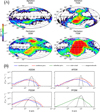 |
Fig. 2 Panels A: set of planetary geographical maps of the solar-wind protons’ precipitation fluxes on the surface for each scenario. Panel B: average energy profiles of the solar-wind protons’ precipitation fluxes for each scenario. The blue lines represent the energy distribution within the northern cusps, the red lines in the southern cusps, and the green line the averaged day-side energy distribution in the case at perihelion with fast solar wind (PFSW). The dashed and dotted lines represent the energy profiles of particle crossing a small window in, respectively, the solar wind and magnetosheath. |
Northern and southern cusp locations and extensions for each scenario.
3.2.2 Energy distribution
The approach adopted here for the evaluation of the precipitating particles fluxes also allows us to gain insight into their energy distribution. The latter is an important parameter for the possible onset of secondary processes such as surface sputtering (e.g. Wurz & Lammer 2003). Each panel in Fig. 2B shows the energy spectrum, in the 10 eV and 10 keV range, of the ions precipitating in the northern regions (blue lines) and the southern regions (red lines) identified in the previous analysis. As for the perihelion FSW case, given its global precipitation spanning the entire subsolar planetary surface, we did not distinguish between northern and southern regions; instead, we considered it as a single whole region (green line). As reference, we also represent the energy spectrum in the solar wind (dashed lines) and in the magnetosheath (dotted lines), which have been computed throughout a window surface totally immersed along the subsolar axis in each related region. The solar-wind energy spectrum represents the typical Maxwellian distribution injected into the box with a peak around 300 eV or 1 keV for the slow and fast solar winds (i.e. 250 and 450 km/s), respectively, with the temperature increasing from aphelion to perihelion. The magnetosheath energy spectrum covers an energy range from 10 eV to 1 keV in the case of SSW, and from a few tens of electronvolts to a few kiloelectronvolts in the case of FSW, showing apeak at a slightly lower energy than the solar wind but a much higher temperature, as expected. It should be noted that a spectrum detection within the magnetosheath requires a careful analysis when its subsolar thickness is compressed.
From these energy spectra, we observe that, in all cases, the northern and southern precipitation profiles are close to the reference magnetosheath energy profile: their peaks are nearly in the same energy band and show comparable values over the entire energy range. This suggests that the majority of the precipitating particles come relatively directly from the magnetosheath region, either from the subsolar point or from the flanks. Additionally, in the first three panels, the precipitation fluxes in the southern regions (red lines) show larger fluxes in the high energy band than those in the northern regions (blue lines).
The precipitation spectra also appear particularly broadened relative to the magnetosheath spectra. This is particularly evident for the perihelion cases (bottom panels), with larger precipitation fluxes in the high and low energy bands. This suggests the presence of additional acceleration or deceleration processes in the interaction with the bow shock and the magnetopause, which are not investigated in this study. Finally, the ion energy distribution is closer to that of the magnetosheath, with a broad spectrum from one electronvolt to a few kiloelectronvolts and a peak at an energy of a few hundred electronvolts, and it is weaker than the solar wind peak.
In the absence of specific observations, the sputtering effect due to the precipitation of solar wind ions on the surface is often assumed to occur from incoming ion energies ≥1 keV, corresponding to a typical solar-wind velocity of about 400 km/s. The results above suggest that the ion energy distribution is closer to that of the magnetosheath, with a broad spectrum from one electronvolt to a few kiloelectronvolts and a peak at an energy of a few hundred electronvolts, and it is weaker than the solar-wind peak.
3.3 Magnetic configuration
Given the strong link between precipitating particles and magnetic configuration, we analysed the magnetic-field topology near and inside the precipitation regions. To do so, we selected an equally distributed number of footprints in these regions and computed the magnetic-field lines starting from them.
In the case of FSW at perihelion, we did not find any closed magnetic-field line inside the large day-side precipitation area. All magnetic field lines detected are open field lines, with their other end extending through the magnetosheath into the interplanetary medium. This suggests that magnetosheath particles have direct access to most of the day-side surface of Mercury.
For the three other cases, we find both open and closed magnetic-field lines. The results are shown in Fig. 3 for each scenario, with the left, middle, and right columns representing the cases of, respectively, SSW at aphelion, FSW at aphelion, and SSW at perihelion. The first and second rows represent the projection in the magnetic equatorial plane of the open field lines (in purple) (i) from the northern cusp region (panels A1–3) and (ii) from the southern cusp region (panels B1–3). In order to better visualise their location in the Hermean environment, they have been superimposed to a grey-coded background representing the magnetic-field map in the magnetic equatorial plane.
Overall, we observe that all open field lines starting from the northern precipitation region (top panels), which are mostly located in the post-noon sector, soon cross the day-side magnetosheath in the pre-noon sector (i.e. dawn side) to continuously extend into this sector of the solar wind. Their configuration in the magnetosheath may become more or less complicated according to the level of turbulence in the foreshock region and in the downstream magnetosheath. This is particularly visible in the FSW case at aphelion (panel A2). We also observe that all open field lines starting from the southern precipitation region (middle panels), which are mostly located in the pre-noon sector, come from the night side and cross the magnetosheath in the post-noon sector (i.e. dusk side).
The bottom panels in Fig. 3 show a view of the closed magnetic-field lines (in blue) from the northern and southern precipitation regions as projected on the terminator plane YZ (Panels C1–3). Their configuration shows a northward shift, as expected from the planetary dipole’s northern shift. They also include a Y component and appear tilted relative to the vertical axis.
Finally, from these latter panels, we can easily infer the boundary between open and closed field lines as the ideal passage between the red dots connected to the blue lines – which represent the footprints of the closed field lines – and those that are not, which instead represent the footprints of the open field lines. As for the northern cusp, this boundary appears nearly aligned along a constant latitude, and its relatively high latitude seen in the aphelion in a SSW case (panel C1) appears to move towards the equator in the related FSW scenario (panel C2) and in the perihelion cases (panel C3). As for the southern cusp, the boundary between open and closed lines exhibits a more oblique orientation featuring high latitudes at pre-noon local times and low latitudes in the noon sector. The southern cusp also appears to move towards the more equatorial latitudes in the cases of FSW at aphelion and SSW at perihelion.
In summary, the magnetic configuration resulting from the interaction of an equatorial and nearly radial IMF, aligned along Parker’s spiral and with a small vertical planetary dipole, produces a very asymmetric configuration in the day-side magnetosphere. This IMF orientation introduces an east-west asymmetry, which adds to the global north-south asymmetry due to the vertical planetary dipole shift. This explains the post-noon (eastwards) shift of the northern cusp and the connection of the corresponding open field lines to the day-side solar wind and magnetosheath. Conversely, the southern cusp is shifted westwards, towards the pre-noon sector, and the related open magnetic-field lines cross a significant section of the night-side and dusk-side magnetosheaths. This behaviour recalls the dawn-dusk asymmetries observed in different parts of the terrestrial magnetosphere including the tail and the plasma sheet, the polar cap, the day-side magnetosphere, and the cusps in response to an equatorial IMF (e.g. Friis-Christensen et al. 1985). As theorised by Cowley (1981b,a), the origin is believed to lie in the fact that the forces exerted by such equatorial IMF on newly open magnetic flux tubes connected to the cusps would include horizontal components. In fact, more recent observations revealed the existence of tilted reconnection lines depending on different clock and cone angles (e.g. Trenchi et al. 2008; Michotte de Welle et al. 2024).
4 Discussion
As shown in Sect. 3, the magnetopause and bow-shock subsolar stand-off distances in the four simulated scenarios appear to be closer to the planet than those predicted by the empirical model proposed by Winslow et al. (2013). One of the possible reasons comes from the fact that the values predicted by the model had to be extrapolated from its analytical formulation, as most of the interplanetary conditions considered here are outside its validity domain. However, this discrepancy also occurs in the case at the aphelion point under FSW, where both the solar-wind dynamic pressure and the Alfvén Mach number lie in its validity range. In fact, apart from the dawn side being disturbed by a large foreshock region, we noticed a significant discrepancy in the sub-solar region, despite the noticeable excellent agreement between the simulated and empirical results shown in all the rest of the domain. In this section, we discuss the possible sources of this difference.
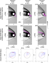 |
Fig. 3 Configuration of magnetic-field lines starting from the cusp regions. The three columns refer to the cases of aphelion SSW, aphelion FSW, and perihelion SSW. The first and second rows represent the pattern of the open magnetic-field lines (purple lines) starting from the northern (panels (A1–3)) and southern (panels (B1–3)) cusps, respectively, as projected on the magnetic equatorial map of the magnetic-field intensity (normalised to the pristine solar wind value). Panels (C1–3) show the closed magnetic-field lines (blue lines) from both the northern and southern solar wind precipitation regions as projected on the YZ terminator plane. The red dots represent the field lines’ footprints; if not associated with any closed field line, they are the footprints of the open field lines shown in Panels A and B. |
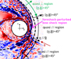 |
Fig. 4 Equatorial subsolar region zoomed-in view of the current density map for the aphelion FSW case shown in Fig. A.1. |
4.1 Role of the quasi-parallel configuration
As already mentioned, the interplanetary magnetic field makes a small angle with respect to the x-axis in the equatorial plane, and it becomes parallel to the bow-shock normal on the equatorial dawn side close to the subsolar point. We illustrate this situation in Fig. 4, with a zoomed-in view of the current density equatorial map (Jz) from Fig. A.1. The angle between the normal of the shock and the IMF remains below 45°, which corresponds to a quasi-parallel configuration, for the whole dawn side. A large foreshock region develops ahead of the bow shock, large disturbances appear in a much thinner magnetosheath and both boundaries are very disturbed. On the contrary, this angle becomes larger than 45° on the dusk side, which corresponds to a quasi-perpendicular configuration (region indicated in green on the map in Fig. 4). In this sector, the boundaries are very clearly defined, and the numerical predictions are well fitted by the empirical model (black dotted lines). In between, the sub-solar region (area pointed out by a purple arrow) corresponds to a quasi-parallel configuration. It still displays some disturbances linked to the nearby foreshock, by marking the transition boundary between both configurations, and resulting in a shorter subsolar stand-off distance than predicted by the model. Hence, we believe that the shorter magnetopause and bow-shock sub-solar stand-off distances predicted by the simulations could be due to a quasi-parallel configuration induced by the IMF orientation in this sector. Moreover, such an asymmetric feature cannot be reproduced by a symmetric paraboloid model as the one considered here.
4.2 Effects of a conductive core and surface
The presence of field-aligned currents in the Hermean magnetosphere has been inferred from MESSENGER observations of the magnetic-field distributions, as well as from active events occurring in the magnetotail (e.g. Anderson et al. 2014, 2018; Dewey 2020). In the absence of an ionosphere, the field-aligned currents can flow within the planetary surface and probably close their path within its conductive core (Janhunen & Kallio 2004; Anderson et al. 2018; Shi et al. 2025a,b). A variation of induced electric currents in regions of high electrical conductivity could in turn produce induced magnetic fields able to affect other global regions, such as the magnetopause. Janhunen & Kallio (2004) analysed the behaviour of the magnetospheric current system under different planetary conductive models with hybrid simulations, finding that asymmetries may occur in the magnetosphere under specific core modelling settings, which include differences in the magnetopause location. Similar results were reached by Jia et al. (2015) from MHD simulations: possible induction effects due to the presence of a differently conductive core may lead to important effects on the magnetopause. However, the quantitatively conductive properties of the inner layers and crust remain inadequately known. In this context, we did not consider any specific planetary conductivity or resistivity formulation. As such, we neglected any possible inductive effects from local current systems developing in proximity to the planetary surface, which could potentially affect the magnetopause, particularly in its subsolar part.
4.3 Impact of the planetary magnetic field
As was done in recent publications (e.g. Fatemi et al. 2020; Shi et al. 2025a), we describe the planetary magnetic field as a pure dipole that is shifted northwards based on what was observed by MESSENGER (Anderson et al. 2011). However, it has been debated that higher order spherical harmonics may possibly contribute significantly ro describing the Hermean magnetosphere (Anderson et al. 2011; Thébault et al. 2018). A modification of the planetary magnetic field would modify the magnetic-field distribution in the magnetosphere, which would in turn affect the type of solar wind - magnetosphere interaction, and consequently the position and shape of the magnetopause.
4.4 Role of the exosphere
One of the characteristics of Mercury is the presence of a tenuous exosphere mainly composed of calcium, featuring a very variable distribution, particularly on the dayside (Milillo et al. 2005; Mangano et al. 2015). This exosphere can be a source of heavy ions. However, MESSENGER in situ observations showed that their density is several orders of magnitude lower than that of the solar wind (Raines et al. 2013), and therefore they are not expected to affect the magnetospheric current system (Exner et al. 2020; Werner et al. 2022). This is why we did not include the presence of an exosphere in the simulations for this study.
5 Conclusions
We performed a set of 3D hybrid simulations to gain a better insight into the effects of the different interplanetary conditions that Mercury encounters along its orbit, especially on its bow shock and magnetosphere, as well as on the solar-wind proton precipitation rates on the surface. In particular, we analysed the specific effects of different interplanetary parameters, such as magnetic field, density and temperature, which increase by a factor of three between the aphelion (at about 0.47 AU) and the perihelion (at about 0.31 AU). For each of these two scenarios, we also examined the role of the solar-wind speed, which, although constant on average at these distances, shows some significant variation between 250 and 450 km/s. This results in the analysis of four cardinal scenarios: at aphelion and perihelion positions under slow (250 km/s) and faster (450 km/s) solar wind conditions.
The values of the interplanetary parameters are chosen based on the results of the recent statistical study in Sun et al. (2022). As for the IMF orientation, we followed the statistics performed by He et al. (2017) and James et al. (2017) from MESSENGER observations, which showed a predominant orientation along the Parker spiral; i.e. in the equatorial plane and with a strong radial component. Thus, we adopted an IMF with an angle of 17° and 25° relative to the Sun-Mercury direction at perihelion and aphelion, respectively. Finally, Mercury’s magnetic field is represented by a vertical magnetic dipole shifted to the north.
The global shapes of the boundaries are found to be generally consistent with those predicted by statistical models (e.g. that proposed in Winslow et al. 2013), with the magnetopause showing a nearly cylindrical shape after 2 RM, and the bow shock with a flaring that decreases with the Alfvénic Mach number. The magnetopause and bow-shock stand-off distances are found in the 1–1.4 RM and 1.3–2 RM ranges, respectively (Table 2). At the perihelion position under FSW, the magnetopause is found almost at the planetary surface. This has already been observed during solar transients (Slavin et al. 2019; Winslow et al. 2020). In addition, our results show that the orientation of the IMF along the Parker spiral induces a dawn-dusk asymmetry, leading to a thinner and disturbed magnetosheath on the dawn side as mainly driven by the quasi-parallel interaction with the bow shock. The fact the subsolar region is also in a quasi-parallel configuration can be one of the reasons why the subsolar bow shock and magnetopause appear closer to the planet than the statistical estimates. Finally, upon comparing all the scenarios with that at the aphelion in SSW (250 km/s), we find that an increase of the solar-wind speed to 450 km/s strongly reduces the stand-off distances of both the bow shock and magnetopause by ~30%. On the contrary, when the planet reaches the perihelion position, this reduction is observed to be much less, that is, ~10%, despite the fact that the interplanetary conditions increased by a factor of three.
We further investigated the precipitation rates of solar-wind protons on the planetary surface, which can represent an important source of energetic particles for secondary mechanisms to occur, such as surface sputtering, which is thought to affect the exosphere dynamics. When the planet is at perihelion and the solar wind is fast, the highest precipitation rates are found in a large region centred at noon on the geographic equator and covering most of the day side (i.e. we found an extension of ~110° latitude and ~90° longitude). This result is due to the magnetopause being close to the surface. Similar precipitation patterns were obtained from simulations with similar solar-wind flows but different orientations of the IMF (Fatemi et al. 2020; Guo et al. 2023).
The other three scenarios show features consistent with observations, such as a cusp location at higher latitudes in the north rather than the south due to the northward shift of the planetary magnetic dipole. We also found latitudinal and longitudinal extensions and precipitation fluxes of the northern cusp in line with previous statistical studies from MESSENGER observations (Winslow et al. 2012; Raines et al. 2022). Knowing the properties of the precipitating particles, we could also infer their energy distributions. We found that the energy distribution in both cusps is comparable to that of the magnetosheath, with possible larger fluxes in the lower and higher energy bands, especially at perihelion. These results are in line with other similar analyses from computer simulations, such as that in Lavorenti et al. (2023). As mentioned in the latter, this spectral broadening may be due to acceleration or deceleration processes at the magnetopause or at the bow shock, the study of which is beyond the scope of this work.
Our results also reveal the following features:
Notable is the local time asymmetry from the noon meridian between the northern and southern cusps. Previous statistical and numerical studies of the northern cusp have generally reported its location to be centred on or around the noon meridian (Winslow et al. 2013; Raines et al. 2022; He et al. 2017; Fatemi et al. 2020). In our three scenarios, the northern and the southern cusps are centred in, respectively, the post-noon sector between 13 and 14.3 LT and the pre-noon sector between and 9 and 10.7 LT. In addition, the southern cusp, expected to cover a larger area than the northern one, exhibits a wide extension towards equatorial latitudes. Surprisingly, its shape departs from an ellipse, as observed for the northern cusp, to the form of a parallelogram inclined in local time from high south latitudes (~45°S) in the pre-noon sector to equatorial latitudes in the post-noon sector with an average width of four hours LT. We suggest that this behaviour is driven by the IMF configuration. In fact, we have shown that, with an IMF aligned along the Parker spiral featuring a large radial component and a small dawn-dusk component, the magnetic configuration appears azimuthally tilted. Open magnetic-field lines from the northern cusp in the post-noon sector extend up to the day-side interplanetary medium through the thin magnetosheath. Conversely, open magnetic-field lines from the southern cusp in the pre-noon sector are connected to the interplanetary medium tailwards through the thick dusk-side magnetosheath. Closed field lines from both cusp regions no longer appear vertical, they are tilted from southern latitudes in the pre-noon sector to northern latitudes in the post-noon sector;
We observe that, in the southern hemisphere, the limit between open and closed field lines also appears very oblique from pre-noon southern latitudes to equatorial post-noon latitudes. We suggest that such an oblique configuration can explain the location and shape of the southern cusps, given the almost identical tilted orientation, while the northern cusp, with an open-closed field line boundary almost aligned along a constant latitude, still presents an elliptic shape elongated in longitude;
Overall, the largest precipitation fluxes in the northern cusp are found at perihelion under SSW conditions, while in the southern hemisphere the largest flux is seen at aphelion under FSW conditions. We observed that these conditions correspond to the location of the closest boundary between open and closed field lines to the equator, whose low latitudes may favour a more efficient penetration of the magnetosheath particles than at higher latitudes.
Such specific features may not have been seen in the statistical studies due to the high variability of the IMF orientation, which could be unknown at the time of the cusp satellites crossing, as well as due to the extremely fast dynamics of Mercury’s environment. In this sense, Raines et al. (2022) highlighted the extreme variability of the cusp fluxes and location from one orbit to another, and even during the same orbit. Simulation studies have examined a wide range of IMF orientations, most of which include either vertical or radial components (e.g. Jia et al. 2019; Fatemi et al. 2020; Aizawa et al. 2022). As such, this study is intended to provide complementary insights into the dynamics of the Hermean environment under specific relevant interplanetary conditions in light of the upcoming observations from the BepiColombo mission.
Acknowledgements
This work was funded by the project Initiative Physique des Infinis (IPI). Simulations were performed using the HPC resources from GENCI (CINES-IDRIS-TGCC) under the grant 2024-A0170410276 on the supercomputer Joliot Curie’s ROME partition, as well as the HPC resources of IDCS support unit from École polytechnique.
Appendix A Maps of magnetic field, particles and current density for each considered scenario to compare with the aphelion SSW case
References
- Aizawa, S., Persson, M., Menez, T., et al. 2022, Planet. Space Sci., 218, 105499 [NASA ADS] [CrossRef] [Google Scholar]
- Anderson, B. J., Johnson, C. L., Korth, H., et al. 2011, Science, 333, 1859 [NASA ADS] [CrossRef] [Google Scholar]
- Anderson, B. J., Johnson, C. L., Korth, H., et al. 2014, Geophys. Res. Lett., 41, 7444 [Google Scholar]
- Anderson, B. J., Johnson, C. L., Korth, H., & Philpott, L. C. 2018, Electric currents in geospace and beyond, 279 [Google Scholar]
- Cazzola, E., Fontaine, D., & Savoini, P. 2023, J. Atmos. Solar-Terrestr. Phys., 246, 106053 [Google Scholar]
- Cowley, S. 1981a, Planet. Space Sci., 29, 809 [Google Scholar]
- Cowley, S. 1981b, Planet. Space Sci., 29, 79 [Google Scholar]
- Dewey, R. M., Slavin, J. A., Raines, J. M., Azari, A. R., & Sun, W. 2020, Journal of Geophysical Research: Space Physics, 125, e2020JA028112 [Google Scholar]
- Dong, C., Wang, L., Hakim, A., et al. 2019, Geophys. Res. Lett., 46, 11584 [NASA ADS] [CrossRef] [Google Scholar]
- Eastwood, J., Lucek, E., Mazelle, C., et al. 2005, Space Sci. Rev., 118, 41 [NASA ADS] [CrossRef] [Google Scholar]
- Exner, W., Simon, S., Heyner, D., & Motschmann, U. 2020, J. Geophys. Res.: Space Phys., 125, e2019JA027691 [CrossRef] [Google Scholar]
- Fatemi, S., Poppe, A., & Barabash, S. 2020, J. Geophys. Res.: Space Phys., 125, e2019JA027706 [Google Scholar]
- Friis-Christensen, E., Kamide, Y., Richmond, A., & Matsushita, S. 1985, J. Geophys. Res.: Space Phys., 90, 1325 [Google Scholar]
- Gedalin, M. 2020, ApJ, 900, 171 [Google Scholar]
- Guo, J., Lu, S., Lu, Q., et al. 2023, J. Geophys. Res.: Planets, 128, e2023JE008032 [Google Scholar]
- He, M., Vogt, J., Heyner, D., & Zhong, J. 2017, J. Geophys. Res.: Space Phys., 122, 6150 [Google Scholar]
- Imber, S. M., & Slavin, J. 2017, J. Geophys. Res.: Space Phys., 122, 11 [Google Scholar]
- James, M. K., Imber, S. M., Bunce, E. J., et al. 2017, J. Geophys. Res.: Space Phys., 122, 7907 [NASA ADS] [CrossRef] [Google Scholar]
- Janhunen, P., & Kallio, E. 2004, in Copernicus Publications Göttingen, Germany, 1829 [Google Scholar]
- Jia, X., Slavin, J. A., Gombosi, T. I., et al. 2015, J. Geophys. Res.: Space Phys., 120, 4763 [NASA ADS] [CrossRef] [Google Scholar]
- Jia, X., Slavin, J. A., Poh, G., et al. 2019, J. Geophys. Res.: Space Phys., 124, 229 [NASA ADS] [CrossRef] [Google Scholar]
- Kallio, E., & Janhunen, P. 2003, in Copernicus Publications Göttingen, Germany, 2133 [Google Scholar]
- Kallio, E., & Janhunen, P. 2004, Adv. Space Res., 33, 2176 [NASA ADS] [CrossRef] [Google Scholar]
- Lapenta, G., Schriver, D., Walker, R. J., et al. 2022, J. Geophys. Res.: Space Phys., 127, e2021JA030241 [Google Scholar]
- Lavorenti, F., Henri, P., Califano, F., et al. 2022, A&A, 664, A133 [NASA ADS] [CrossRef] [EDP Sciences] [Google Scholar]
- Lavorenti, F., Jensen, E. A., Aizawa, S., et al. 2023, Planet. Sci. J., 4, 163 [Google Scholar]
- Leblanc, F., & Johnson, R. 2003, Icarus, 164, 261 [Google Scholar]
- Leblanc, F., & Johnson, R. E. 2010, Icarus, 209, 280 [Google Scholar]
- Livesey, W., Kennel, C., & Russell, C. 1982, Geophys. Res. Lett., 9, 1037 [NASA ADS] [CrossRef] [Google Scholar]
- Mangano, V., Massetti, S., Milillo, A., et al. 2015, Planet. Space Sci., 115, 102 [Google Scholar]
- Michotte de Welle, B., Aunai, N., Lavraud, B., et al. 2024, Front. Astron. Space Sci., 11, 1427791 [Google Scholar]
- Milillo, A., Wurz, P., Orsini, S., et al. 2005, Space Sci. Rev., 117, 397 [CrossRef] [Google Scholar]
- Modolo, R., Hess, S., Mancini, M., et al. 2016, J. Geophys. Res. (Space Phys.), 121, 6378 [Google Scholar]
- Moissard, C., Fontaine, D., & Savoini, P. 2019, J. Geophys. Res.: Space Phys., 124, 8208 [NASA ADS] [CrossRef] [Google Scholar]
- Moses, S., Coroniti, F., & Scarf, F. 1988, Geophys. Res. Lett., 15, 429 [NASA ADS] [CrossRef] [Google Scholar]
- Orsini, S., Mangano, V., Milillo, A., et al. 2018, Sci. Rep., 8, 928 [Google Scholar]
- Raines, J. M., Gershman, D. J., Zurbuchen, T. H., et al. 2013, Journal of Geophysical Research: Space Physics, 118, 1604 [Google Scholar]
- Raines, J. M., Dewey, R. M., Staudacher, N. M., et al. 2022, J. Geophys. Res.: Space Phys., 127, e2022JA030397 [Google Scholar]
- Richer, E., Modolo, R., Chanteur, G. M., Hess, S., & Leblanc, F. 2012, J. Geophys. Res. (Space Phys.), 117, A10228 [Google Scholar]
- Romanelli, N., Modolo, R., Leblanc, F., et al. 2018, J. Geophys. Res. (Space Phys.), 123, 5315 [Google Scholar]
- Scudder, J., Burlaga, L., & Greenstadt, E. 1984, J. Geophys. Res.: Space Phys., 89, 7545 [Google Scholar]
- Shi, Z., Fatemi, S., Rong, Z., He, F., & Wei, Y. 2025a, Icarus, 438, 116633 [Google Scholar]
- Shi, Z., Rong, Z., Fatemi, S., et al. 2025b, J. Geophys. Res.: Planets, 130, e2024JE008610 [Google Scholar]
- Slavin, J. A., Lepping, R. P., Wu, C.-C., et al. 2010, Geophys. Res. Lett., 37, L02105 [Google Scholar]
- Slavin, J. A., DiBraccio, G. A., Gershman, D. J., et al. 2014, J. Geophys. Res.: Space Phys., 119, 8087 [NASA ADS] [CrossRef] [Google Scholar]
- Slavin, J., Middleton, H., Raines, J., et al. 2019, J. Geophys. Res.: Space Phys., 124, 6613 [Google Scholar]
- Sun, W., Dewey, R. M., Aizawa, S., et al. 2022, Sci. China Earth Sci., 65, 25 [NASA ADS] [CrossRef] [Google Scholar]
- Thébault, E., Langlais, B., Oliveira, J., Amit, H., & Leclercq, L. 2018, Phys. Earth Planet. Interiors, 276, 93 [Google Scholar]
- Trenchi, L., Marcucci, M., Pallocchia, G., et al. 2008, J. Geophys. Res.: Space Phys., 113, A07S10 [Google Scholar]
- Turc, L., Fontaine, D., Savoini, P., & Modolo, R. 2015, J. Geophys. Res. (Space Phys.), 120, 6133 [Google Scholar]
- Walsh, A. P., Haaland, S., Forsyth, C., et al. 2014, in Copernicus GmbH, 705 [Google Scholar]
- Werner, A., Aizawa, S., Leblanc, F., et al. 2022, Icarus, 372, 114734 [Google Scholar]
- Winslow, R. M., Johnson, C. L., Anderson, B. J., et al. 2012, Geophys. Res. Lett., 39, GL051472 [Google Scholar]
- Winslow, R. M., Anderson, B. J., Johnson, C. L., et al. 2013, J. Geophys. Res.: Space Phys., 118, 2213 [Google Scholar]
- Winslow, R. M., Johnson, C. L., Anderson, B. J., et al. 2014, Geophys. Res. Lett., 41, 4463 [Google Scholar]
- Winslow, R. M., Philpott, L., Paty, C. S., et al. 2017, J. Geophys. Res.: Space Phys., 122, 4960 [Google Scholar]
- Winslow, R. M., Lugaz, N., Philpott, L., et al. 2020, ApJ, 889, 184 [Google Scholar]
- Wurz, P., & Lammer, H. 2003, Icarus, 164, 1 [Google Scholar]
- Zurbuchen, T. H., Raines, J. M., Slavin, J. A., et al. 2011, Science, 333, 1862 [Google Scholar]
All Tables
Values of magnetopause and bow shock’s stand-off distances on magnetic equator from simulations.
All Figures
|
Fig. 1 Aphelion SSW scenario. Upper panels show a cross-section in the meridian plane (at Y = 0 km), while lower panels show a cross-section along the magnetic equatorial plane (at Z = 484 km). Each row shows the maps of the magnetic-field intensity, B, the current components (JZ in upper panel and JY in lower panel), and the particle density. The dotted black lines represent the predicted magnetopause and bow shock’s shapes based on the model proposed in Winslow et al. (2013). The Sun is ideally located on the right edge, and the solar wind flows from the right edge to left. |
| In the text | |
|
Fig. 2 Panels A: set of planetary geographical maps of the solar-wind protons’ precipitation fluxes on the surface for each scenario. Panel B: average energy profiles of the solar-wind protons’ precipitation fluxes for each scenario. The blue lines represent the energy distribution within the northern cusps, the red lines in the southern cusps, and the green line the averaged day-side energy distribution in the case at perihelion with fast solar wind (PFSW). The dashed and dotted lines represent the energy profiles of particle crossing a small window in, respectively, the solar wind and magnetosheath. |
| In the text | |
|
Fig. 3 Configuration of magnetic-field lines starting from the cusp regions. The three columns refer to the cases of aphelion SSW, aphelion FSW, and perihelion SSW. The first and second rows represent the pattern of the open magnetic-field lines (purple lines) starting from the northern (panels (A1–3)) and southern (panels (B1–3)) cusps, respectively, as projected on the magnetic equatorial map of the magnetic-field intensity (normalised to the pristine solar wind value). Panels (C1–3) show the closed magnetic-field lines (blue lines) from both the northern and southern solar wind precipitation regions as projected on the YZ terminator plane. The red dots represent the field lines’ footprints; if not associated with any closed field line, they are the footprints of the open field lines shown in Panels A and B. |
| In the text | |
|
Fig. 4 Equatorial subsolar region zoomed-in view of the current density map for the aphelion FSW case shown in Fig. A.1. |
| In the text | |
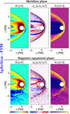 |
Fig. A.1 Aphelion FSW scenario. Same format as Fig. 1. |
| In the text | |
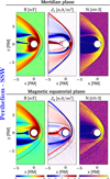 |
Fig. A.2 Perihelion SSW scenario. Same format as Fig. 1. |
| In the text | |
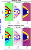 |
Fig. A.3 Perihelion FSW scenario. Same format as Fig. 1. |
| In the text | |
Current usage metrics show cumulative count of Article Views (full-text article views including HTML views, PDF and ePub downloads, according to the available data) and Abstracts Views on Vision4Press platform.
Data correspond to usage on the plateform after 2015. The current usage metrics is available 48-96 hours after online publication and is updated daily on week days.
Initial download of the metrics may take a while.