| Issue |
A&A
Volume 701, September 2025
|
|
|---|---|---|
| Article Number | A234 | |
| Number of page(s) | 11 | |
| Section | Extragalactic astronomy | |
| DOI | https://doi.org/10.1051/0004-6361/202553996 | |
| Published online | 18 September 2025 | |
Noema formIng Cluster survEy (NICE): A census of star formation and cold gas properties in massive protoclusters at 1.5 < z < 4
1
School of Astronomy and Space Science, Nanjing University, Nanjing 210093, China
2
Key Laboratory of Modern Astronomy and Astrophysics (Nanjing University), Ministry of Education, Nanjing 210093, China
3
AIM, CEA, CNRS, Université Paris-Saclay, Université Paris Diderot, Sorbonne Paris Cité, F-91191 Gif-sur-Yvette France
4
, IRAM, 300 rue de la piscine, F-38406 Saint-Martin d’Hères, France
5
Cosmic Dawn Center (DAWN), Jagtvej 128, DK2200 Copenhagen N, Denmark
6
DTU-Space, Technical University of Denmark, Elektrovej 327, 2800 Kgs. Lyngby, Denmark
7
Max-Planck-Institut für Extraterrestrische Physik (MPE), Giessenbachstrasse 1, 85748 Garching, Germany
8
School of Mathematics and Physics, Anqing Normal University, Anqing 246133, China
9
Institute of Astronomy and Astrophysics, Anqing Normal University, Anqing 246133, China
10
Purple Mountain Observatory, Chinese Academy of Sciences, 10 Yuanhua Road, Nanjing 210023, China
11
Niels Bohr Institute, University of Copenhagen, Jagtvej 128, DK-2200 Copenhagen N, Denmark
12
Instituto de Astrofísica de Canarias, C. Vía Láctea, s/n, 38205 La Laguna, Tenerife, Spain
13
Universidad de La Laguna, Dpto. Astrofísica, 38206 La Laguna, Tenerife, Spain
14
European Southern Observatory, Karl-Schwarzschild-Str. 2, D-85748 Garching bei Munchen, Germany
15
Steward Observatory, University of Arizona, 933 N. Cherry Avenue, Tucson, AZ 85721, USA
16
INAF – Osservatorio di Astrofisica e Scienza dello Spazio di Bologna, Via Gobetti 93/3, I-40129 Bologna, Italy
17
Department of Astronomy, University of Geneva, Chemin Pegasi 51, 1290 Versoix, Switzerland
18
Instituto de Física, Pontificia Universidad Católica de Valparaíso, Casilla 4059, Valparaíso, Chile
19
INAF – Osservatorio Astronomico di Trieste, Via Tiepolo 11, 34131 Trieste, Italy
20
IFPU – Institute for Fundamental Physics of the Universe, Via Beirut 2, 34014 Trieste, Italy
21
Department of Physics, University of Helsinki, Gustaf Hällströmin katu 2, FI-00014 Helsinki, Finland
22
Department of Physics & Astronomy, University of California Los Angeles, 430 Portola Plaza, Los Angeles, CA 90095, USA
23
Chinese Academy of Sciences South America Center for Astronomy, National Astronomical Observatories, CAS, Beijing 100101, China
⋆ Corresponding authors: This email address is being protected from spambots. You need JavaScript enabled to view it.
; This email address is being protected from spambots. You need JavaScript enabled to view it.
Received:
2
February
2025
Accepted:
8
July
2025
Abstract
Massive protoclusters at z ∼ 1.5 − 4, the peak of the cosmic star formation history, are key to understanding the formation mechanisms of massive galaxies in today’s clusters. However, studies of protoclusters at these high redshifts remain limited, primarily due to small sample sizes and heterogeneous selection criteria. For this work, we conducted a systematic investigation of the star formation and cold gas properties of member galaxies of eight massive protoclusters in the COSMOS field, using the statistical and homogeneously selected sample from the Noema formIng Cluster survEy (NICE). Our analysis reveals a steep increase in the star formation rates per halo mass (ΣSFR/Mhalo) with redshifts in these intensively star-forming protoclusters, reaching values one to two orders of magnitude higher than those observed in the field at z > 2. We further show that instead of an enhancement of starbursts, this increase is largely driven by the concentration of massive and gas-rich star-forming galaxies in the protocluster cores. The member galaxies still generally follow the same star-forming main sequence as in the field, with a moderate enhancement at the low-mass end. Notably, the most massive protocluster galaxies (M⋆ > 8×10¹⁰ M⊙) exhibit higher μgas and τgas than their field counterparts, while remaining on the star-forming main sequence. These gas-rich, massive, and star-forming galaxies are predominantly concentrated in the protocluster cores and are likely progenitors of massive ellipticals in the center of today’s clusters. These results suggest that the formation of massive galaxies in such environments is sustained by substantial gas reservoirs, which in turn support persistent star formation and drive early mass assembly in forming cluster cores.
Key words: galaxies: clusters: general / galaxies: evolution / galaxies: high-redshift / galaxies: starburst
© The Authors 2025
 Open Access article, published by EDP Sciences, under the terms of the Creative Commons Attribution License (https://creativecommons.org/licenses/by/4.0), which permits unrestricted use, distribution, and reproduction in any medium, provided the original work is properly cited.
This article is published in open access under the Subscribe to Open model. This email address is being protected from spambots. You need JavaScript enabled to view it. to support open access publication.
1. Introduction
The environmental influence on the progenitors of massive galaxies in local clusters is critical for understanding the formation of these galaxies (Peng et al. 2010; Behroozi et al. 2019; van der Burg et al. 2020). Over the past decade, extensive studies of massive protoclusters at the peak of the cosmic star formation history (z ∼ 2 − 4), selected through various methods, have been inconclusive in producing an unambiguous consistent picture of the environmental effects on star formation and cold gas properties of galaxies in these structures (e.g., Rudnick et al. 2017; Gómez-Guijarro et al. 2019; Jin et al. 2023, 2024; Bakx et al. 2024; Pensabene et al. 2024). Specifically, some structures show a prevalence of submillimeter galaxies (SMGs) or ultra-luminous infrared galaxies (LIRGs), suggesting enhanced star formation in their galaxies as compared to average field environments (e.g., Casey 2016; Wang et al. 2016; Oteo et al. 2018). Other studies, primarily based on Hα emitters in protoclusters, report little to no difference in the star-forming main sequence (SFMS) compared to their field counterparts (e.g, Valentino et al. 2015; Shimakawa et al. 2018; Pérez-Martínez et al. 2023). Molecular gas is the fuel for star formation. The well-established star formation law (Kennicutt 1998; Gao & Solomon 2004) highlights the role of internal secular processes in the conversion of cold gas into stars. Additionally, a bimodal scenario has been proposed to describe the observed offset between starburst galaxies and normal star-forming galaxies, where starburst galaxies show higher star formation efficiency (SFE), which may result from a higher merger rate or a more compact distribution of molecular gas, among other factors (Daddi et al. 2010; Sargent et al. 2014; Liu et al. 2019).
In dense environments, increased interactions can compress gas, thus enhancing SFEs, while cold gas inflows through filaments connected to protoclusters can replenish gas reservoirs, thus sustaining high gas fractions. Deep CO observations of cluster galaxies z ∼ 1.6 reveal a consistent or enhanced gas fraction compared to the field counterparts (Rudnick et al. 2017; Noble et al. 2017). In the Spiderweb protocluster at z = 2.15, Dannerbauer et al. (2017) identified a massive and extended CO(1–0) disk around the central radio galaxies. Follow-up analysis by Pérez-Martínez et al. (2025) revealed a decreasing gas fraction with increasing stellar mass, showing a particularly steep decline above log(M⋆/M⊙) = 10.5. In CL J1001, a starbusting protocluster at z = 2.51, Wang et al. (2018) observed decreasing gas fractions toward the cluster center, suggesting the imminent formation of a passive core by z ∼ 2. Tadaki et al. (2019) found a declining gas fraction and gas depletion time with increasing stellar mass in galaxies in three protoclusters traced by radio galaxies at z ∼ 2, and suggested that gas accretion is accelerated in less massive galaxies and suppressed in more massive ones. At even higher redshifts (z ≳ 4), extreme starbusting protocluster cores such as SPT2349-56 and Distant Red Core (DRC) exhibit lower gas fractions compared to field SMGs (Long et al. 2020; Hill et al. 2022). Nevertheless, there is a paucity of protoclusters at high redshift with deep multi-wavelength coverage to comprehensively link the stellar and gas properties of member galaxies. Such observations are essential for revealing the physical mechanisms driving the formation of massive galaxies in these dense environments.
The Noema formIng Cluster survEy (NICE, Zhou et al. 2024) is a 159-hour NOEMA Large Program (ID: M21AA, PIs: E. Daddi and T. Wang) targeting 48 massive protocluster candidates across multiple fields, complemented by a 40-h ALMA program (ID: 2021.1.00815.S) focusing on 25 southern candidates. The primary goal of these programs is to spectroscopically confirm protoclusters at cosmic noon through CO emission from their member galaxies, significantly expanding the sample size in this field of research. Notably, eight protoclusters at 1.5 < z < 4 have been confirmed in the COSMOS field (Sillassen et al. 2024). The COSMOS field provides extensive ancillary data across optical, near-infrared (NIR), far-infrared (FIR), submillimeter, and radio wavelengths (Weaver et al. 2022; Jin et al. 2018; Smolčić et al. 2017), which, combined with the CO observations from the NICE survey, offer a unique opportunity to investigate the environmental impact on galaxy evolution.
For this paper we investigated the star formation activity and cold gas content of eight massive protoclusters in the COSMOS field, identified through the NICE survey (hereafter NICE-COSMOS). Our analysis focuses on the protoclusters’ central region (within one virial radius), as detailed in the following sections. We adopt a standard ΛCDM cosmology with H0 = 70 km s−1 Mpc−1, Ωm = 0.3, and ΩΛ = 0.7, and a Chabrier (2003) initial mass function.
2. Data
2.1. NICE-COSMOS protoclusters
The eight protoclusters in NICE-COSMOS, along with their member identification, are detailed in Sillassen et al. (2024). Briefly, the members are selected with |zphot–zspec, group| < 0.1(1 + zspec, group) within a virial projected radius based on the COSMOS2020 catalog (Weaver et al. 2022). The NICE survey selects intensively star-forming massive protoclusters at 2 ≲ z ≲ 4, which are chosen as overdensities of high-z massive galaxies traced by red IRAC sources in association with SPIRE-350 μm peakers that show intense star formation. We list the selection criteria here:
(1) Overdensity of red IRAC sources:
![Mathematical equation: $$ \begin{aligned} \begin{aligned}{[3.6] - [4.5]} &> 0.1 \,; \\ 20 < [4.5]&< 23 \,; \\ \Sigma _N&> 5\sigma \, \text{(N} \text{=} \text{5} \text{ or} \text{10)}. \end{aligned} \end{aligned} $$](/articles/aa/full_html/2025/09/aa53996-25/aa53996-25-eq1.gif) (1)
(1)
[3.6], [4.5] are IRAC magnitudes from COSMOS2020 (Weaver et al. 2022), and ΣN =  is the Nth closest neighbor density estimator, where dN is the distance to the Nth closest galaxy.
(2) SPIRE-350μm peakers:
 (2)
(2)
S250, S350, and S500 are the Herschel/SPIRE fluxes at 250 μm, 350 μm, and 500μm.
Figure A.1 shows the spatial distribution of all members including CO and continuum detections in the eight protoclusters in NICE-COSMOS, which are primarily concentrated at the cluster centers. For the following analysis, we focus on galaxies within one virial radius, 1Rvir, as defined in Sillassen et al. (2024), as this area is also well covered by the NOEMA and ALMA observations. The virial radii range from 141 pkpc to 429 pkpc, and the number of member galaxies per structure varies between 13 and 31.
According to the selection method, the NICE protoclusters are traced by intensively star-forming massive galaxies, which are likely to undergo a more active formation phase driven by enhanced gas reservoirs, elevated merger rates, or other physical processes, compared to protoclusters selected through alternative methods.
2.2. Stellar masses and star formation rates
We used stellar masses and star formation rates (SFRs) derived with LePhare (Arnouts et al. 2002) in COSMOS2020 (Weaver et al. 2022). For galaxies detected in the FIR, specifically those in the super-deblended catalog (Jin et al. 2018), we also explored various SFR tracers to obtain accurate measurements.
We first cross-matched the members in the super-deblended catalog (Jin et al. 2018) with a separation smaller than 1″. The matches have a median separation of 0.15″. Notably, the 3GHz and 24 μm fluxes are measured directly at the galaxy positions, hence the risk of misidentification or flux misattribution is substantially reduced. For galaxies detected at 3 GHz (Smolčić et al. 2017) with a signal-to-noise ratio (S/N) greater than 3, we calculated the SFR from LIR (Kennicutt 1998), as derived from the 3 GHz radio emission. This was done using the infrared radio correlation (IRRC, qIR(z, M⋆), Delvecchio et al. 2021) and a spectral index of α = –0.8. The high spatial resolution (0.75″) of the VLA 3 GHz observations helps mitigate blending issues in crowded regions, which can affect FIR flux measurements. For sources with S/N3 GHz < 3, we computed LIR from 24 μm fluxes using the conversion from Wuyts et al. (2008). The results are listed in Table 1.
Properties of the CO or continuum-detected galaxies in the massive protoclusters of NICE-COSMOS.
As we show in Fig. 1, SFRradio and SFR24 μm are consistent. For galaxy 839791 in COSMOS-SBC6, which has a radio luminosity twice that of the crossover luminosity described in Wang et al. (2024), the threshold above which radio emission is dominated by AGN, we used SFR24 μm to minimize the contamination from AGN-related radio emission.
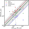 |
Fig. 1. Comparison of SFRs derived from radio emission with those derived using other methods. The comparison includes SFRs estimated from Wuyts et al. (2008, green), deblended FIR fluxes from Jin et al. (2018, red), SFRs derived with LEPHARE as in COSMOS2020 ((Weaver et al. 2022), blue), and SFRs scaled from overall average SEDs of the protoclusters to dust continuum (black). Only galaxies with S/N3GHz > 3 are shown. The black solid line represents a 1:1 relation, while the shaded region indicates the 0.2 dex uncertainties. The dashed colored lines show the median ratios between SFRradio and the SFRs derived from the fours different methods, respectively: 0.90, 1.81, 0.37, 1.57. |
In addition, we calculated SFRs by scaling the total LIR derived from the best-fit SED of the integrated FIR photometry of each protocluster (Sillassen et al. 2024) to the dust continuum emission of individual members, assuming the same dust temperature for all members. We find that the scaled SFR is generally 1.6 times higher than SFRradio; this is more prominent for those galaxies with SFRradio ∼ 100 M⊙ yr−1, while galaxies with higher SFRradio have similarly scaled SFRs.
Overall, we conclude that using SFRradio does not change the conclusion of this paper.
2.3. Gas masses
The molecular gas mass is converted from the Rayleigh-Jeans dust continuum at 850 μm,  , as calibrated with the prescription in Hughes et al. (2017). This method leverages dust continuum emission, which is intrinsically associated with gas in the entire cold molecular gas reservoir (Genzel et al. 2015; Scoville et al. 2016), and offers a much more sensitive measure than high-J CO emission, which primarily traces the dense gas phase only (Liu et al. 2015; Daddi et al. 2015; Valentino et al. 2020) and has limited detections due to the narrow line width compared to continuum observations. The dust continuum at 3 mm and 2 mm from the NOEMA and ALMA observations of the NICE survey, closely corresponding to rest-frame 850 μm for the cluster galaxies, was used to derive gas masses. The NOEMA and ALMA observations have average angular resolutions of 4.1″and 0.7″, respectively. For spatially resolved sources, we used a Gaussian model to fit the visibilities. Unresolved sources were modeled as point sources.
We also estimated the gas masses from CO(3–2) or CO(4–3) line emission,  , by converting them to the ground-state CO(1–0) luminosity, assuming the CO spectral line energy distribution (CO-SLED) of star-forming galaxies at z = 2.0–2.7 from the ASPECS survey (Boogaard et al. 2020). These galaxies exhibit slightly higher CO excitation compared to main sequence galaxies at z < 2 (Valentino et al. 2020), but overall agree, within the uncertainties, with the average SLEDs of SMGs at z = 1.2 – 4.8 (Birkin et al. 2021). The conversion factor αCO was derived using the mass–SFR–metallicity relation from Genzel et al. (2015) and the metallicity dependence of αCO from Tacconi et al. (2018) for our sample.
In Fig. 2 we compare the gas masses estimated using the two methods. The two methods yield consistent results within 0.3 dex, with  approximately 1.5 times higher than
  . A similar comparison of CO(1–0) and 1.2 mm dust continuum measurements in galaxies within the Spiderweb protocluster also shows comparable results, albeit with large scatters (Zhang et al. 2024). Table 1 lists the αCO values and gas masses calculated with different tracers. For consistency, in the following we adopt gas masses estimated from the dust continuum.
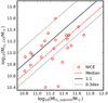 |
Fig. 2. Comparison of the gas mass derived from CO emission lines and dust continuum. The black line denotes the one-to-one relation and the dotted lines show the 0.3 dex uncertainties. The NICE sample are circles, and the median ratio of −0.18 dex is indicated by the dashed line. |
3. Star formation and cold gas properties
3.1. Enhanced Star Formation in Massive Halos in the Early Universe
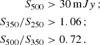
The value of ΣSFR/Mhalo in clusters increases with redshift, following an empirical relation of (1+z)n (see Alberts & Noble 2022 for a review). The NICE survey extends such studies to z > 2. We adopted the integrated SFR and best estimates of halo masses of the eight protoclusters from Sillassen et al. (2024) to obtain the total SFR per unit halo mass (ΣSFR/Mhalo). The SFR is from the FIR spectral energy distribution (SED) fitting using the dust templates in Magdis et al. (2012), and the halo masses are the average results from six methods including stellar mass-to-halo mass relations, overdensity with galaxy bias, and NFW profile fitting to radial stellar mass density. In Fig. 3 we include the eight massive protoclusters in NICE-COSMOS; LH-SBC3 at z = 3.95, which is the most distant protocluster identified in the NICE survey (Zhou et al. 2024); protoclusters RO1001 at z = 2.91 (Kalita et al. 2021) and CL J1001 at z = 2.51 (Wang et al. 2018), which are prototypes within the NICE survey; and SPT2349-56 at z = 4.3 (Hill et al. 2022) and Distant Red Core at z = 4.0 (Long et al. 2020), which are starbursting protoclusters similar to the NICE clusters. We found that ΣSFR/Mhalo increases by an order of magnitude from z = 2 to z = 4, following the evolutionary trend observed in galaxy clusters up to z = 1 (ΣSFR/Mhalo ∝ (1+z)5.4, Webb et al. 2013), which has recently been shown to extend to clusters at z = 1.6–2 (Smail 2024). These values are one to two orders of magnitude higher than those observed in the field (∝ (1+z)3 − 4 Sargent et al. 2012; Ilbert et al. 2013, 2015). This may be due to the evolution of the SFMS, modulated by the evolution of the M⋆, tot/Mhalo relation, and the reduction of the quenched fraction (Elias et al. in prep.).
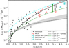 |
Fig. 3. Total SFR per unit halo mass as a function of redshift. Shown as red circles are the eight massive protoclusters in the COSMOS field and LH-SBC3 at z = 3.95, the most distant protocluster identified in the NICE survey (Zhou et al. 2024), as well as two other prototypes within the NICE survey, RO1001 at z = 2.91 (Kalita et al. 2021) and CL J1001 at z = 2.51 (Wang et al. 2018). Two other starbursting protoclusters, SPT2349-56 at z = 4.3 (Hill et al. 2022) and Distant Red Core at z = 4.0 (Long et al. 2020), are shown as a cyan square and diamond, respectively. CGG-z4, a compact galaxy group at z = 4.3 in the COSMOS field (Brinch et al. 2025), is shown as a cyan circle. The black dots and the curves show the (proto)clusters and redshift evolution compiled in Alberts & Noble (2022). The (proto)cluster data are drawn from Haines et al. (2013), Santos et al. (2014, 2015), Popesso et al. (2015a,b), Ma et al. (2015), Alberts et al. (2014, 2016), Casey (2016), Strazzullo et al. (2018), Smith et al. (2019), Lacaille et al. (2019). The black dashed line shows a redshift evolution trend ∝z1.77 (Popesso et al. 2011), while the green dash-dotted line indicates a ∝(1 + z)5.4 relation (Alberts et al. 2014; Webb et al. 2013; Bai et al. 2009). The cyan dash-dotted line also follows the ∝(1 + z)5.4 trend, but is scaled from logM200/M⊙ = 14.5 to 14, assuming ΣSFR/ |
3.2. Star-forming main sequence in dense environments
The SFR and stellar mass of all UVJ-active cluster members (Williams et al. 2009) are shown in Fig. 4. Galaxies at different redshifts are scaled to z = 2.5, following the SFMS normalization and redshift evolution from Schreiber et al. (2015). Despite significant scatter, the median values of these galaxies closely follow the main sequence in the field, in line with the results from Hα emitters in protoclusters at z ∼ 2.5 (e.g., Spiderweb, Pérez-Martínez et al. 2023).
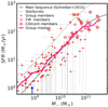 |
Fig. 4. Star-forming main sequence of galaxy members in the eight protoclusters within NICE-COSMOS. CO-detected and dust continuum-detected members are highlighted with open red circles, while other FIR-detected galaxies are marked with open red squares. The remaining cluster members are represented as red dots. To enable comparison, the galaxies are scaled to a common redshift of z = 2.5, using the SFMS normalization and redshift evolution from Schreiber et al. (2015). The SFRs of FIR-detected members are derived from 3 GHz radio emission or 24 μm fluxes, while the SFRs for the rest are obtained from COSMOS2020 (see Section 2.2 for details). The pink curve represents the median SFR of member galaxies within the NICE-COSMOS protoclusters. For reference, the black solid curve shows the main sequence at z = 2.5 from Schreiber et al. (2015), and the dotted curve indicates the starburst regime, defined as RSB = 4 (Rodighiero et al. 2011). The blue arrow indicates the mass completeness limit of star-forming galaxies at z = 2.5 from COSMOS2020 (Weaver et al. 2022). |
The CO-detected members, which are among the most massive with the highest SFRs, may indicate a greater abundance of gas fueling star formation in these galaxies. However, this trend is not observed in the CO-detected Hα emitters in the Spiderweb protocluster (Pérez-Martínez et al. 2025), where SFRs are derived from the dust-corrected Hα fluxes, possibly due to the differences in protocluster selection criteria. In contrast, the less massive galaxies display slightly elevated star formation compared to field galaxies, a trend similar to that observed in Hα emitters within the young protocluster USS1558-003 at z = 2.53 (Hayashi et al. 2012; Daikuhara et al. 2024).
It is important to note that the cluster members were primarily selected based on photometric redshifts, which may include interlopers. This may affect the results shown in Fig. 4, especially at the low-mass end, where the contamination is most significant. On the other hand, the high-mass end is less impacted as it is dominated by CO-detected galaxies that are spectroscopically confirmed members.
3.3. Build-up of massive galaxies in the dense cores
We analyzed the stellar mass distribution of the cluster galaxies and found that more massive galaxies are located closer to the protocluster center (Fig. 5a). The median stellar mass within 0.1 Rvir is ∼1010.6 M⊙, compared to ∼109.5 M⊙ at the outskirts, representing more than 1 dex difference. This difference in the mass of main sequence galaxies naturally enhances the overall star formation activities in these protoclusters. Out of the 31 massive galaxies (M⋆ > 3 × 10¹⁰ M⊙), 21 are located within 0.3Rvir, with all but one showing detected CO emission. This aligns with the high fraction of SMGs predicted in protocluster cores by Araya-Araya et al. (2024) simulations and highlights the presence of substantial gas reservoirs in these regions. Similarly, a top-heavy stellar mass function has been identified in the starbursting protocluster CL J1001 (Sun et al. 2024), suggesting a prevalence of massive galaxy accumulation in such protoclusters. Although these massive galaxies generally follow the main sequence, those in the cores are on average situated above the main sequence compared to their counterparts in the outskirts (Fig. 5b).
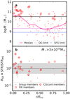 |
Fig. 5. Panel a: Stellar mass as a function of distance to the cluster centers. The symbols are as defined in Fig. 4. The completeness limits of star-forming galaxies and quiescent galaxies are also shown as references. Panel b: Starburstiness (RSB) of massive galaxies (M⋆ > 3 × 10¹⁰ M⊙) as a function of the distance to the cluster center. The dashed line shows the field main sequence and the shaded region shows the uncertainty. |
The field of view (FoV) of the NOEMA and ALMA observations, with a full width at half maximum (FWHM) of ∼30″and ∼1′, respectively, is sufficiently large to encompass the area within the virial radius of the protoclusters. This indicates that we are witnessing the rapid build-up of massive galaxies in the cores of these protoclusters at cosmic noon.
3.4. Gas content
The gas masses of CO-detected NICE-COSMOS galaxies span the range Mgas = 1010.6 ∼ 1011.7 M⊙. The gas-to-stellar mass ratio μgas = Mgas/M⋆ and gas depletion time τgas = Mgas/SFR of NICE protocluster galaxies have median values of μgas, NICE = 1.32 and τgas, NICE = 0.78 Gyr. These values are consistent with those observed in other protocluster galaxies at similar redshifts (e.g., Tadaki et al. 2019; Pérez-Martínez et al. 2025). However, protoclusters at higher redshifts (z ≳ 4), such as SPT2349-56 (Hill et al. 2022) and LH-SBC3 (Zhou et al. 2024), tend to show lower μgas and τgas, while massive galaxies in Distant Red Core at z = 4 (Long et al. 2020) have comparable gas content to those in protoclusters at z ∼ 2.5. For a fair comparison, we recalculated the gas masses of galaxies in the literature using the same method described in Section 2.3 when CO(1–0) measurements were unavailable.
To assess the environmental impact on the gas content, we normalized μgas and τgas to the corresponding field levels, accounting for their dependence on stellar mass, starburstiness, and redshift. This analysis utilized parameterized relations compiled from the A3COSMOS project, based on a systematic mining of ALMA archival data for CO-observed galaxies in the COSMOS field (Liu et al. 2019). The results are presented in Fig. 6.
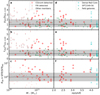 |
Fig. 6. Gas-to-stellar mass ratio (μgas = Mgas/M⋆), gas depletion time (τgas = Mgas/SFR), and starburstiness (RSB) as a function of stellar mass (left column) and redshift (right column). μgas and τgas are scaled relative to field galaxy levels (μgas, scale, τgas, scale), accounting for the stellar masses, redshifts, and starburstiness of each galaxy. The red circles represent galaxies detected in CO or dust continuum in the NICE protoclusters, including the eight in the COSMOS field (Sillassen et al. 2024), LH-SBC3 (Zhou et al. 2024), RO1001 (Kalita et al. 2021), and CL J1001 (Wang et al. 2018), while red squares and dots indicate the 3σ upper limits of those detected in the FIR and the rest of the cluster galaxies. Two additional starbursting protoclusters at z ≳ 4, SPT2349-56 (Hill et al. 2022) and Distant Red Core (Long et al. 2020), are shown in cyan. Field galaxies from Kaasinen et al. (2019), Boogaard et al. (2020), Frias Castillo et al. (2023) are represented as green triangles, with the molecular gas content derived from CO(1–0) emission lines. The black dashed lines denote the positions of field galaxies; the gray shading indicates the uncertainties. |
The 3σ detection limit of the NICE observations corresponds to a gas mass of Mgas ∼ 1011 M⊙ for galaxies at z ∼ 2.5, meaning that our sample predominantly includes the most massive members and the less massive galaxies with high starburstiness (Fig. 6c). The most massive ones (M⋆ > 1010.8 M⊙), which are concentrated in the core regions, are nearly all detected via CO or dust continuum emission. These massive galaxies generally exhibit higher gas content (∼2×) compared to their counterparts in the field (Figs. 6a, b). Several of them display significantly elevated gas-to-stellar mass ratios and gas depletion times relative to field galaxies. However, their SFRs are not correspondingly enhanced, suggesting that they have abundant gas reservoirs to sustain their growth or their SFRs are prevented from increasing to starburst levels due to merger-related processes or negative feedback.
We also note that the field galaxies (Kaasinen et al. 2019; Boogaard et al. 2020; Frias Castillo et al. 2023), whose molecular gas content is derived from CO(1–0) emission adopting αCO obtained using the method outlined in Section 2.3, fall within the field-level range defined by the A3COSMOS project. This is consistent with the findings from Calvi et al. (2023), who found a correlation between molecular gas masses of SMGs and the significance of the associated overdensity.
Most galaxies with lower stellar masses are not detected in CO or dust continuum, except for the starbursts. However, these starburst galaxies exhibit gas-to-stellar mass ratios and gas depletion times comparable to those of field galaxies. It remains unclear whether the CO- or dust-nondetected cluster members have enhanced or deficient gas content.
In contrast, three protoclusters traced by Lyα emitters and/or red galaxies surrounding a radio galaxy (Tadaki et al. 2019) show the opposite trend, with a declining gas fraction and gas depletion time as stellar mass increases. This indicates a mass-dependent environmental effect, where gas accretion is accelerated in less massive galaxies, while suppressed in more massive ones. These contrasting trends may reflect different evolutionary stages of the two protocluster populations.
Interestingly, we find that most of the gas-rich galaxies belong to protoclusters at z ∼ 2.5, whereas massive galaxies in more distant protoclusters exhibit a declining gas content, though still generally within the uncertainties of field galaxies (Fig. 6d,e), approximately 2 times at z = 2.5 and 1.2 times at z = 4. Similarly, Calvi et al. (2023) identified a possible transitioning phase at z ∼ 4, with z < 4 protoclusters more populated by dusty galaxies. We speculate that our observed trend may partly reflect a selection bias in constructing the field sample, which tends to favor the brightest sources at high redshifts, typically located in dense environments.
We further checked the overall mean intensity of the radiation field, ⟨U⟩, of the NICE-COSMOS protoclusters, as measured from the integrated FIR SED fitting in Sillassen et al. (2024). ⟨U⟩ can be used to infer the metallicity weighted star formation efficiency (SFE ≡1/τgas) and is proportional to dust temperature (Magdis et al. 2012, 2017). The evolution of ⟨U⟩ with redshift for the eight protoclusters generally follows the trend observed in main sequence galaxies (Béthermin et al. 2015); a few of them show lower ⟨U⟩. This is in line with the moderately longer gas depletion time observed in the individual member galaxies and may indicate a colder dust temperature in these protoclusters (see Fig. 7).
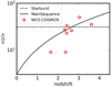 |
Fig. 7. Evolution of the mean intensity of the radiation field, ⟨U⟩, with redshift. The red circles show the overall ⟨U⟩ of the eight protoclusters in NICE-COSMOS. The solid curve and dashed line represent the trend of main sequence galaxies and starbursts, as in Béthermin et al. (2015). |
4. Summary and discussion
In this paper we analyzed the star formation and cold gas properties of eight protoclusters in the COSMOS field, selected through the NICE survey, which targets intensively star-forming protocluster cores at cosmic noon.
We find that the total SFR per unit halo mass (ΣSFR/Mhalo) in protoclusters at z > 2 increases rapidly with redshift, scaling as (1 + z)5.4 (Fig. 3). This could be due to either a higher number of massive star-forming galaxies in massive halos or enhanced star formation in cluster galaxies. Additionally, we find that the fraction of quiescent galaxies decreases relative to that observed in lower-redshift (proto)clusters, and that the streaming mass of the halos (i.e., the threshold mass delimiting the hot and cold in hot accretion regimes; see Daddi et al. 2022 and Dekel et al. 2009) is also a good predictor for the quiescent fraction, making the gas accretion mode a potential explanation for the quiescent fraction evolution across halos (Elias et al. in prep.). We also caution that the higher ΣSFR/Mhalo values at higher redshifts could also be partly driven by lower halo masses. Nevertheless, this rise in star formation activity in protoclusters is not reflected in individual member galaxies. The SFMS remains comparable to that observed in the field (Fig. 4), suggesting that the elevated ΣSFR/Mhalo in protoclusters is not driven by a higher fraction of starburst galaxies in dense environments. We note that the cluster members may be affected by contamination due to photometric redshift uncertainties (Sillassen et al. 2024). However, the massive end is dominated by CO-detected and thus spectroscopically confirmed members, making the main sequence at the high-mass end less susceptible to interlopers.
Using observations from NOEMA and ALMA in the NICE survey, we investigated the gas content of cluster galaxies. The CO or dust continuum-detected galaxies are predominantly massive cluster members (M⋆ > 3×10¹⁰ M⊙), which preferentially reside in the core of the protoclusters (r ≲ 0.3Rvir, Fig. 5). This indicates an overabundance of massive star-forming galaxies in these protocluster cores, which contributes to their elevated ΣSFR/Mhalo. This finding aligns with the simulations by Araya-Araya et al. (2024), which identify an excess of massive star-forming galaxies undergoing a submillimeter-bright phase in protocluster cores, suggesting a downsizing formation scenario for massive galaxies.
In terms of stellar-to-gas mass ratio and gas depletion time, the median values are consistent with field levels. However, the most massive galaxies (M⋆ > 8 × 10¹⁰ M⊙) are notably more gas-rich than their field counterparts (Fig. 6). This suggests efficient cold gas accretion in the central regions of these protoclusters, supporting the growth of these galaxies to higher masses while remaining in the main sequence mode, without triggering starburst phases. For the less massive galaxies, CO or dust continuum detections are limited to the most starbursting ones, which follow the scaling relation (μgas(z, M⋆, RSB), τgas(z, M⋆, RSB), Liu et al. 2019) observed in the field galaxies. The moderately higher τgas is consistent with the overall mean intensity of the radiation field in the protoclusters, indicating a generally cold dust temperature in these dense environments. However, we caution that the NICE survey is biased toward protoclusters in active star-forming phases. The influence of such environments on member galaxies may differ from that observed in protoclusters selected through other methods.
Acknowledgments
We thank the anonymous referee for valuable comments. This work was supported by National Natural Science Foundation of China (Project Nos. 13001103, 12173017 and Key Project No.12141301), National Key R&D Program of China (grant no. 2023YFA1605600), Scientific Research Innovation Capability Support Project for Young Faculty (Project No. ZYGXQNJSKYCXNLZCXM-P3), and the China Manned Space Program with grant no. CMS-CSST-2025-A04. L.Z. and Y.S. acknowledges the support from the National Key R&D Program of China No. 2022YFF0503401 and 2018YFA0404502, the National Natural Science Foundation of China (NSFC grants 12141301, 12121003, 11825302). Y.S. thanks the support by the New Cornerstone Science Foundation through the XPLORER PRIZE. Y.J.W. acknowledges support by National Natural Science Foundation of China (Project No. 12403019) and Jiangsu Natural Science Foundation (Project No. BK20241188). GEM acknowledges the Villum Fonden research grant 13160 “Gas to stars, stars to dust: tracing star formation across cosmic time”, grant 37440, “The Hidden Cosmos”, and the Cosmic Dawn Center of Excellence funded by the Danish National Research Foundation under the grant No. 140. CGG acknowledges support from CNES. ZJ acknowledges funding from JWST/NIRCam contract to the University of Arizona NAS5-02015. ID acknowledges funding by the INAF Minigrant “Harnessing the power of VLBA toward a census of AGN and star formation at high redshift” and by the European Union – NextGenerationEU, RRF M4C2 1.1, Project 2022JZJBHM: “AGN-sCAN: zooming-in on the AGN-galaxy connection since the cosmic noon” – CUP C53D23001120006. CdE acknowledges funding from the MCIN/AEI (Spain) and the “NextGenerationEU”/PRTR (European Union) through the Juan de la Cierva-Formación program (FJC2021-047307-I). SJ is supported by the European Union’s Horizon Europe research and innovation program under the Marie Skłodowska-Curie grant agreement No. 101060888. This research used APLpy, an open-source plotting package for Python (Robitaille & Bressert 2012; Robitaille 2019). This work is based on observations carried out under project number M21AA with the IRAM NOEMA Interferometer. IRAM is supported by INSU/CNRS (France), MPG (Germany) and IGN (Spain). This research uses data obtained through the Telescope Access Program (TAP), which is funded by the National Astronomical Observatories, Chinese Academy of Sciences, and the Special Fund for Astronomy from the Ministry of Finance. This work is based on observations obtained with WIRCam, a joint project of CFHT, Taiwan, Korea, Canada, France, at the Canada-France-Hawaii Telescope (CFHT) which is operated by the National Research Council (NRC) of Canada, the Institute National des Sciences de l’Univers of the Centre National de la Recherche Scientifique of France, and the University of Hawaii.
References
- Alberts, S., & Noble, A. 2022, Universe, 8, 554 [Google Scholar]
- Alberts, S., Pope, A., Brodwin, M., et al. 2014, MNRAS, 437, 437 [NASA ADS] [CrossRef] [Google Scholar]
- Alberts, S., Pope, A., Brodwin, M., et al. 2016, ApJ, 825, 72 [NASA ADS] [CrossRef] [Google Scholar]
- Araya-Araya, P., Cochrane, R. K., Hayward, C. C., et al. 2024, ApJ, 977, 204 [Google Scholar]
- Arnouts, S., Moscardini, L., Vanzella, E., et al. 2002, MNRAS, 329, 355 [Google Scholar]
- Bai, L., Rieke, G. H., Rieke, M. J., Christlein, D., & Zabludoff, A. I. 2009, ApJ, 693, 1840 [NASA ADS] [CrossRef] [Google Scholar]
- Bakx, T. J. L. C., Berta, S., Dannerbauer, H., et al. 2024, MNRAS, 530, 4578 [NASA ADS] [CrossRef] [Google Scholar]
- Behroozi, P., Wechsler, R. H., Hearin, A. P., & Conroy, C. 2019, MNRAS, 488, 3143 [NASA ADS] [CrossRef] [Google Scholar]
- Béthermin, M., Daddi, E., Magdis, G., et al. 2015, A&A, 573, A113 [Google Scholar]
- Birkin, J. E., Weiss, A., Wardlow, J. L., et al. 2021, MNRAS, 501, 3926 [Google Scholar]
- Biviano, A., Fadda, D., Durret, F., Edwards, L. O. V., & Marleau, F. 2011, A&A, 532, A77 [NASA ADS] [CrossRef] [EDP Sciences] [Google Scholar]
- Boogaard, L. A., van der Werf, P., Weiss, A., et al. 2020, ApJ, 902, 109 [NASA ADS] [CrossRef] [Google Scholar]
- Brinch, M., Jin, S., Gobat, R., et al. 2025, A&A, 694, A218 [NASA ADS] [CrossRef] [EDP Sciences] [Google Scholar]
- Calvi, R., Castignani, G., & Dannerbauer, H. 2023, A&A, 678, A15 [NASA ADS] [CrossRef] [EDP Sciences] [Google Scholar]
- Casey, C. M. 2016, ApJ, 824, 36 [CrossRef] [Google Scholar]
- Casey, C. M., Kartaltepe, J. S., Drakos, N. E., et al. 2023, ApJ, 954, 31 [NASA ADS] [CrossRef] [Google Scholar]
- Chabrier, G. 2003, ApJ, 586, L133 [NASA ADS] [CrossRef] [Google Scholar]
- Cowie, L. L., Barger, A. J., Fomalont, E. B., & Capak, P. 2004, ApJ, 603, L69 [Google Scholar]
- Daddi, E., Elbaz, D., Walter, F., et al. 2010, ApJ, 714, L118 [NASA ADS] [CrossRef] [Google Scholar]
- Daddi, E., Dannerbauer, H., Liu, D., et al. 2015, A&A, 577, A46 [NASA ADS] [CrossRef] [EDP Sciences] [Google Scholar]
- Daddi, E., Rich, R. M., Valentino, F., et al. 2022, ApJ, 926, L21 [NASA ADS] [CrossRef] [Google Scholar]
- Daikuhara, K., Kodama, T., Pérez-Martínez, J. M., et al. 2024, MNRAS, 531, 2335 [NASA ADS] [CrossRef] [Google Scholar]
- Dannerbauer, H., Lehnert, M. D., Emonts, B., et al. 2017, A&A, 608, A48 [NASA ADS] [CrossRef] [EDP Sciences] [Google Scholar]
- Dekel, A., Birnboim, Y., Engel, G., et al. 2009, Nature, 457, 451 [Google Scholar]
- Delvecchio, I., Daddi, E., Sargent, M. T., et al. 2021, A&A, 647, A123 [NASA ADS] [CrossRef] [EDP Sciences] [Google Scholar]
- Frias Castillo, M., Hodge, J., Rybak, M., et al. 2023, ApJ, 945, 128 [NASA ADS] [CrossRef] [Google Scholar]
- Gao, Y., & Solomon, P. M. 2004, ApJ, 606, 271 [NASA ADS] [CrossRef] [Google Scholar]
- Geach, J. E., Smail, I., Ellis, R. S., et al. 2006, ApJ, 649, 661 [NASA ADS] [CrossRef] [Google Scholar]
- Genzel, R., Tacconi, L. J., Lutz, D., et al. 2015, ApJ, 800, 20 [Google Scholar]
- Gómez-Guijarro, C., Riechers, D. A., Pavesi, R., et al. 2019, ApJ, 872, 117 [CrossRef] [Google Scholar]
- Haines, C. P., Pereira, M. J., Smith, G. P., et al. 2013, ApJ, 775, 126 [NASA ADS] [CrossRef] [Google Scholar]
- Hayashi, M., Kodama, T., Tadaki, K.-I., Koyama, Y., & Tanaka, I. 2012, ApJ, 757, 15 [NASA ADS] [CrossRef] [Google Scholar]
- Hill, R., Chapman, S., Phadke, K. A., et al. 2022, MNRAS, 512, 4352 [NASA ADS] [CrossRef] [Google Scholar]
- Hughes, T. M., Ibar, E., Villanueva, V., et al. 2017, MNRAS, 468, L103 [NASA ADS] [CrossRef] [Google Scholar]
- Ilbert, O., McCracken, H. J., Le Fèvre, O., et al. 2013, A&A, 556, A55 [NASA ADS] [CrossRef] [EDP Sciences] [Google Scholar]
- Ilbert, O., Arnouts, S., Le Floc’h, E., et al. 2015, A&A, 579, A2 [NASA ADS] [CrossRef] [EDP Sciences] [Google Scholar]
- Jin, S., Daddi, E., Liu, D., et al. 2018, ApJ, 864, 56 [Google Scholar]
- Jin, S., Sillassen, N. B., Magdis, G. E., et al. 2023, A&A, 670, L11 [NASA ADS] [CrossRef] [EDP Sciences] [Google Scholar]
- Jin, S., Sillassen, N. B., Magdis, G. E., et al. 2024, A&A, 683, L4 [NASA ADS] [CrossRef] [EDP Sciences] [Google Scholar]
- Kaasinen, M., Scoville, N., Walter, F., et al. 2019, ApJ, 880, 15 [NASA ADS] [CrossRef] [Google Scholar]
- Kalita, B. S., Daddi, E., D’Eugenio, C., et al. 2021, ApJ, 917, L17 [NASA ADS] [CrossRef] [Google Scholar]
- Kennicutt, R. C., Jr 1998, ApJ, 498, 541 [Google Scholar]
- Lacaille, K. M., Chapman, S. C., Smail, I., et al. 2019, MNRAS, 488, 1790 [NASA ADS] [CrossRef] [Google Scholar]
- Le Floc’h, E., Papovich, C., Dole, H., et al. 2005, ApJ, 632, 169 [Google Scholar]
- Liu, D., Gao, Y., Isaak, K., et al. 2015, ApJ, 810, L14 [NASA ADS] [CrossRef] [Google Scholar]
- Liu, D., Schinnerer, E., Groves, B., et al. 2019, ApJ, 887, 235 [Google Scholar]
- Long, A. S., Cooray, A., Ma, J., et al. 2020, ApJ, 898, 133 [NASA ADS] [CrossRef] [Google Scholar]
- Ma, C. J., Smail, I., Swinbank, A. M., et al. 2015, ApJ, 806, 257 [Google Scholar]
- Magdis, G. E., Daddi, E., Béthermin, M., et al. 2012, ApJ, 760, 6 [NASA ADS] [CrossRef] [Google Scholar]
- Magdis, G. E., Rigopoulou, D., Daddi, E., et al. 2017, A&A, 603, A93 [NASA ADS] [CrossRef] [EDP Sciences] [Google Scholar]
- Noble, A. G., McDonald, M., Muzzin, A., et al. 2017, ApJ, 842, L21 [Google Scholar]
- Oteo, I., Ivison, R. J., Dunne, L., et al. 2018, ApJ, 856, 72 [Google Scholar]
- Peng, Y.-J., Lilly, S. J., Kovač, K., et al. 2010, ApJ, 721, 193 [Google Scholar]
- Pensabene, A., Cantalupo, S., Cicone, C., et al. 2024, A&A, 684, A119 [NASA ADS] [CrossRef] [EDP Sciences] [Google Scholar]
- Pérez-Martínez, J. M., Dannerbauer, H., Kodama, T., et al. 2023, MNRAS, 518, 1707 [Google Scholar]
- Pérez-Martínez, J. M., Dannerbauer, H., Emonts, B. H. C., et al. 2025, A&A, 696, A236 [NASA ADS] [CrossRef] [EDP Sciences] [Google Scholar]
- Popesso, P., Rodighiero, G., Saintonge, A., et al. 2011, A&A, 532, A145 [NASA ADS] [CrossRef] [EDP Sciences] [Google Scholar]
- Popesso, P., Biviano, A., Finoguenov, A., et al. 2015a, A&A, 579, A132 [NASA ADS] [CrossRef] [EDP Sciences] [Google Scholar]
- Popesso, P., Biviano, A., Finoguenov, A., et al. 2015b, A&A, 574, A105 [NASA ADS] [CrossRef] [EDP Sciences] [Google Scholar]
- Robitaille, T. 2019, https://doi.org/10.5281/zenodo.2567476 [Google Scholar]
- Robitaille, T., & Bressert, E. 2012, Astrophysics Source Code Library [record ascl:1208.017] [Google Scholar]
- Rodighiero, G., Daddi, E., Baronchelli, I., et al. 2011, ApJ, 739, L40 [Google Scholar]
- Rudnick, G., Hodge, J., Walter, F., et al. 2017, ApJ, 849, 27 [NASA ADS] [CrossRef] [Google Scholar]
- Rujopakarn, W., Eisenstein, D. J., Rieke, G. H., et al. 2010, ApJ, 718, 1171 [NASA ADS] [CrossRef] [Google Scholar]
- Santos, J. S., Altieri, B., Tanaka, M., et al. 2014, MNRAS, 438, 2565 [NASA ADS] [CrossRef] [Google Scholar]
- Santos, J. S., Altieri, B., Valtchanov, I., et al. 2015, MNRAS, 447, L65 [NASA ADS] [CrossRef] [Google Scholar]
- Sargent, M. T., Béthermin, M., Daddi, E., & Elbaz, D. 2012, ApJ, 747, L31 [Google Scholar]
- Sargent, M. T., Daddi, E., Béthermin, M., et al. 2014, ApJ, 793, 19 [NASA ADS] [CrossRef] [Google Scholar]
- Schreiber, C., Pannella, M., Elbaz, D., et al. 2015, A&A, 575, A74 [NASA ADS] [CrossRef] [EDP Sciences] [Google Scholar]
- Scoville, N., Sheth, K., Aussel, H., et al. 2016, ApJ, 820, 83 [Google Scholar]
- Shimakawa, R., Kodama, T., Hayashi, M., et al. 2018, MNRAS, 473, 1977 [NASA ADS] [CrossRef] [Google Scholar]
- Sillassen, N. B., Jin, S., Magdis, G. E., et al. 2022, A&A, 665, L7 [NASA ADS] [CrossRef] [EDP Sciences] [Google Scholar]
- Sillassen, N. B., Jin, S., Magdis, G. E., et al. 2024, A&A, 690, A55 [NASA ADS] [CrossRef] [EDP Sciences] [Google Scholar]
- Smail, I. 2024, MNRAS, 529, 2290 [Google Scholar]
- Smith, C. M. A., Gear, W. K., Smith, M. W. L., Papageorgiou, A., & Eales, S. A. 2019, MNRAS, 486, 4304 [CrossRef] [Google Scholar]
- Smolčić, V., Novak, M., Delvecchio, I., et al. 2017, A&A, 602, A6 [NASA ADS] [CrossRef] [EDP Sciences] [Google Scholar]
- Strazzullo, V., Coogan, R. T., Daddi, E., et al. 2018, ApJ, 862, 64 [NASA ADS] [CrossRef] [Google Scholar]
- Sun, H., Wang, T., Xu, K., et al. 2024, ApJ, 967, L34 [NASA ADS] [CrossRef] [Google Scholar]
- Tacconi, L. J., Genzel, R., Saintonge, A., et al. 2018, ApJ, 853, 179 [Google Scholar]
- Tadaki, K.-I., Kodama, T., Hayashi, M., et al. 2019, PASJ, 71, 40 [NASA ADS] [CrossRef] [Google Scholar]
- Valentino, F., Daddi, E., Strazzullo, V., et al. 2015, ApJ, 801, 132 [NASA ADS] [CrossRef] [Google Scholar]
- Valentino, F., Daddi, E., Puglisi, A., et al. 2020, A&A, 641, A155 [NASA ADS] [CrossRef] [EDP Sciences] [Google Scholar]
- van der Burg, R. F. J., Rudnick, G., Balogh, M. L., et al. 2020, A&A, 638, A112 [NASA ADS] [CrossRef] [EDP Sciences] [Google Scholar]
- Wang, T., Elbaz, D., Daddi, E., et al. 2016, ApJ, 828, 56 [NASA ADS] [CrossRef] [Google Scholar]
- Wang, T., Elbaz, D., Daddi, E., et al. 2018, ApJ, 867, L29 [NASA ADS] [CrossRef] [Google Scholar]
- Wang, Y., Wang, T., Liu, D., et al. 2024, A&A, 685, A79 [NASA ADS] [CrossRef] [EDP Sciences] [Google Scholar]
- Weaver, J. R., Kauffmann, O. B., Ilbert, O., et al. 2022, ApJS, 258, 11 [NASA ADS] [CrossRef] [Google Scholar]
- Webb, T. M. A., O’Donnell, D., Yee, H. K. C., et al. 2013, AJ, 146, 84 [NASA ADS] [CrossRef] [Google Scholar]
- Williams, R. J., Quadri, R. F., Franx, M., van Dokkum, P., & Labbé, I. 2009, ApJ, 691, 1879 [NASA ADS] [CrossRef] [Google Scholar]
- Wuyts, S., Labbé, I., Förster Schreiber, N. M., et al. 2008, ApJ, 682, 985 [NASA ADS] [CrossRef] [Google Scholar]
- Zhang, Y. H., Dannerbauer, H., Pérez-Martínez, J. M., et al. 2024, A&A, 692, A22 [NASA ADS] [CrossRef] [EDP Sciences] [Google Scholar]
- Zhou, L., Wang, T., Daddi, E., et al. 2024, A&A, 684, A196 [NASA ADS] [CrossRef] [EDP Sciences] [Google Scholar]
Appendix A: NICE-COSMOS images
 |
Fig. A.1. RGB images of the eight protoclusters in the COSMOS field identified in the NICE survey. The color channels are R: [4.5], G: Ks, B: Y, except for the two protoclusters covered by COSMOS-Web (Casey et al. 2023), COSMOS-SBC4 and COSMOS-SBCX3, where the color channels are R: F444W, G: F277W, B: F150W. Each image has a size of 1′×1′. The red, yellow, and cyan circles highlight the CO-detected members, spectroscopically confirmed members, and all other members identified by Sillassen et al. (2024), respectively. |
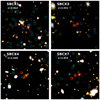 |
Fig. A.1. continued. |
All Tables
Properties of the CO or continuum-detected galaxies in the massive protoclusters of NICE-COSMOS.
All Figures
|
Fig. 1. Comparison of SFRs derived from radio emission with those derived using other methods. The comparison includes SFRs estimated from Wuyts et al. (2008, green), deblended FIR fluxes from Jin et al. (2018, red), SFRs derived with LEPHARE as in COSMOS2020 ((Weaver et al. 2022), blue), and SFRs scaled from overall average SEDs of the protoclusters to dust continuum (black). Only galaxies with S/N3GHz > 3 are shown. The black solid line represents a 1:1 relation, while the shaded region indicates the 0.2 dex uncertainties. The dashed colored lines show the median ratios between SFRradio and the SFRs derived from the fours different methods, respectively: 0.90, 1.81, 0.37, 1.57. |
| In the text | |
|
Fig. 2. Comparison of the gas mass derived from CO emission lines and dust continuum. The black line denotes the one-to-one relation and the dotted lines show the 0.3 dex uncertainties. The NICE sample are circles, and the median ratio of −0.18 dex is indicated by the dashed line. |
| In the text | |
|
Fig. 3. Total SFR per unit halo mass as a function of redshift. Shown as red circles are the eight massive protoclusters in the COSMOS field and LH-SBC3 at z = 3.95, the most distant protocluster identified in the NICE survey (Zhou et al. 2024), as well as two other prototypes within the NICE survey, RO1001 at z = 2.91 (Kalita et al. 2021) and CL J1001 at z = 2.51 (Wang et al. 2018). Two other starbursting protoclusters, SPT2349-56 at z = 4.3 (Hill et al. 2022) and Distant Red Core at z = 4.0 (Long et al. 2020), are shown as a cyan square and diamond, respectively. CGG-z4, a compact galaxy group at z = 4.3 in the COSMOS field (Brinch et al. 2025), is shown as a cyan circle. The black dots and the curves show the (proto)clusters and redshift evolution compiled in Alberts & Noble (2022). The (proto)cluster data are drawn from Haines et al. (2013), Santos et al. (2014, 2015), Popesso et al. (2015a,b), Ma et al. (2015), Alberts et al. (2014, 2016), Casey (2016), Strazzullo et al. (2018), Smith et al. (2019), Lacaille et al. (2019). The black dashed line shows a redshift evolution trend ∝z1.77 (Popesso et al. 2011), while the green dash-dotted line indicates a ∝(1 + z)5.4 relation (Alberts et al. 2014; Webb et al. 2013; Bai et al. 2009). The cyan dash-dotted line also follows the ∝(1 + z)5.4 trend, but is scaled from logM200/M⊙ = 14.5 to 14, assuming ΣSFR/ |
| In the text | |
|
Fig. 4. Star-forming main sequence of galaxy members in the eight protoclusters within NICE-COSMOS. CO-detected and dust continuum-detected members are highlighted with open red circles, while other FIR-detected galaxies are marked with open red squares. The remaining cluster members are represented as red dots. To enable comparison, the galaxies are scaled to a common redshift of z = 2.5, using the SFMS normalization and redshift evolution from Schreiber et al. (2015). The SFRs of FIR-detected members are derived from 3 GHz radio emission or 24 μm fluxes, while the SFRs for the rest are obtained from COSMOS2020 (see Section 2.2 for details). The pink curve represents the median SFR of member galaxies within the NICE-COSMOS protoclusters. For reference, the black solid curve shows the main sequence at z = 2.5 from Schreiber et al. (2015), and the dotted curve indicates the starburst regime, defined as RSB = 4 (Rodighiero et al. 2011). The blue arrow indicates the mass completeness limit of star-forming galaxies at z = 2.5 from COSMOS2020 (Weaver et al. 2022). |
| In the text | |
|
Fig. 5. Panel a: Stellar mass as a function of distance to the cluster centers. The symbols are as defined in Fig. 4. The completeness limits of star-forming galaxies and quiescent galaxies are also shown as references. Panel b: Starburstiness (RSB) of massive galaxies (M⋆ > 3 × 10¹⁰ M⊙) as a function of the distance to the cluster center. The dashed line shows the field main sequence and the shaded region shows the uncertainty. |
| In the text | |
|
Fig. 6. Gas-to-stellar mass ratio (μgas = Mgas/M⋆), gas depletion time (τgas = Mgas/SFR), and starburstiness (RSB) as a function of stellar mass (left column) and redshift (right column). μgas and τgas are scaled relative to field galaxy levels (μgas, scale, τgas, scale), accounting for the stellar masses, redshifts, and starburstiness of each galaxy. The red circles represent galaxies detected in CO or dust continuum in the NICE protoclusters, including the eight in the COSMOS field (Sillassen et al. 2024), LH-SBC3 (Zhou et al. 2024), RO1001 (Kalita et al. 2021), and CL J1001 (Wang et al. 2018), while red squares and dots indicate the 3σ upper limits of those detected in the FIR and the rest of the cluster galaxies. Two additional starbursting protoclusters at z ≳ 4, SPT2349-56 (Hill et al. 2022) and Distant Red Core (Long et al. 2020), are shown in cyan. Field galaxies from Kaasinen et al. (2019), Boogaard et al. (2020), Frias Castillo et al. (2023) are represented as green triangles, with the molecular gas content derived from CO(1–0) emission lines. The black dashed lines denote the positions of field galaxies; the gray shading indicates the uncertainties. |
| In the text | |
|
Fig. 7. Evolution of the mean intensity of the radiation field, ⟨U⟩, with redshift. The red circles show the overall ⟨U⟩ of the eight protoclusters in NICE-COSMOS. The solid curve and dashed line represent the trend of main sequence galaxies and starbursts, as in Béthermin et al. (2015). |
| In the text | |
|
Fig. A.1. RGB images of the eight protoclusters in the COSMOS field identified in the NICE survey. The color channels are R: [4.5], G: Ks, B: Y, except for the two protoclusters covered by COSMOS-Web (Casey et al. 2023), COSMOS-SBC4 and COSMOS-SBCX3, where the color channels are R: F444W, G: F277W, B: F150W. Each image has a size of 1′×1′. The red, yellow, and cyan circles highlight the CO-detected members, spectroscopically confirmed members, and all other members identified by Sillassen et al. (2024), respectively. |
| In the text | |
|
Fig. A.1. continued. |
| In the text | |
Current usage metrics show cumulative count of Article Views (full-text article views including HTML views, PDF and ePub downloads, according to the available data) and Abstracts Views on Vision4Press platform.
Data correspond to usage on the plateform after 2015. The current usage metrics is available 48-96 hours after online publication and is updated daily on week days.
Initial download of the metrics may take a while.