| Issue |
A&A
Volume 701, September 2025
|
|
|---|---|---|
| Article Number | A105 | |
| Number of page(s) | 11 | |
| Section | Planets, planetary systems, and small bodies | |
| DOI | https://doi.org/10.1051/0004-6361/202554415 | |
| Published online | 05 September 2025 | |
Non-linear evolution of the unstratified polydisperse dust settling instability
Faculty of Aerospace Engineering, Delft University of Technology,
Kluyverweg 1,
2629
HS
Delft,
The Netherlands
★ Corresponding author: This email address is being protected from spambots. You need JavaScript enabled to view it.
Received:
7
March
2025
Accepted:
14
July
2025
Abstract
Context. The dust settling instability (DSI) is a member of the resonant drag instability family, and is thus related to the streaming instability (SI). Linear calculations found that the unstratified monodisperse DSI has growth rates much higher than the SI even with lower initial dust-to-gas ratios. However, recent non-linear investigation found no evidence of strong dust clumping at the saturation level.
Aims. We seek to investigate the non-linear saturation of the mono- and polydisperse DSI. We examine the convergence behaviour with regard to both the numerical resolution as well as the number of species. By characterising the morphology of the dust evolution triggered by the DSI, we can shed more light on its role in planetesimal formation.
Methods. We performed a suite of 2D shearing box hydrodynamic simulations with the code IDEFIX, both in the mono- and polydisperse regimes. We focussed on the time evolution of the maximum dust density, noting the time at which the instability is triggered, and analysed the morphology of the resultant structure.
Results. In our monodisperse DSI simulations, the maximum dust density increases and the instability saturates earlier with a higher spatial resolution, with no signs of convergence yet. The polydisperse simulations do seem to converge with the number of species and produce maximum dust densities that are comparable to, albeit lower than, the monodisperse simulations. Different dust species tend to form adjacent but separate dust filaments, which may have implications on dust growth and further clumping.
Conclusions. The monodisperse DSI produces dust structure at densities high enough to likely lead to clumping. The polydisperse DSI produces lower but comparable dust densities at the same spatial resolution. Our idealised treatment suggests that the DSI is important for planetesimal formation, as it is less affected by the inclusion of a dust size distribution than the SI.
Key words: accretion, accretion disks / hydrodynamics / instabilities / methods: numerical / planets and satellites: formation
© The Authors 2025
 Open Access article, published by EDP Sciences, under the terms of the Creative Commons Attribution License (https://creativecommons.org/licenses/by/4.0), which permits unrestricted use, distribution, and reproduction in any medium, provided the original work is properly cited.
This article is published in open access under the Subscribe to Open model. This email address is being protected from spambots. You need JavaScript enabled to view it. to support open access publication.
1 Introduction
Planet formation theory requires dust to grow in proto-planetary discs from micron-sized particles, as inherited from the interstellar medium, to kilometre-sized planetesimals in less than 10 Myr. Dust growth by coagulation is efficient for small particles, but the process halts once dust grows to centimetre-sized pebbles due to the radial drift Weidenschilling (1977) as well as the bouncing and fragmentation barriers (Blum & Wurm 2008). Safronov (1969) and Goldreich & Ward (1973) independently proposed a shortcut to this approach, whereby dust settling into a gravitationally unstable thin layer leads to the direct formation of planetesimals. However, it was soon found out that this settling causes vertical shear that triggers turbulence at a level that prevents the formation of the dense thin dust layer (Weidenschilling 1980).
The current understanding of planet formation relies on dust instabilities as a means to increase dust densities and form self-gravitating clumps (Chiang & Youdin 2010). The streaming instability (SI) (Youdin & Goodman 2005; Youdin & Johansen 2007; Johansen & Youdin 2007) is widely seen as the favourite mechanism to accomplish this. While simulations with single species show that the SI is capable of producing high-density dust clumps (Johansen et al. 2007), multi-species SI with a dust size distribution seem to face some challenges. Krapp et al. (2019) found linear growth rates for discrete multi-species SI that are much lower than the ones for single species. Paardekooper et al. (2020) showed that the SI vanishes in parts of the wave number space when approaching the continuous size distribution limit. In the non-linear regime, Yang & Zhu (2021) found that growth is still possible for a multi-species SI when the dust-to-gas ratio, μ, exceeds unity (see also Matthijsse et al. 2025).
The resonant drag instability (RDI) framework was recently put forward as a way to derive a family of instabilities that occur at low dust-to-gas ratio, μ (Squire & Hopkins 2018b,a). RDIs develop when the gas supports a wave with a phase velocity that matches the (projected) streaming velocity of dust particles through the gas. This resonance leads to linear instability, often causing fast growth of the dust density perturbations. The choice of gas wave and dust streaming determines the type of RDI: sound waves lead to the acoustic RDI (Squire & Hopkins 2018b; Magnan et al. 2024a), while inertial waves lead to either the streaming or settling instability (Squire & Hopkins 2018a; Magnan et al. 2024b), depending on the direction of the dust drift. The newly identified dust settling instability (DSI) was found to grow much faster in the linear regime and required a lower initial μ than the SI Squire & Hopkins (2018a); Zhuravlev (2019).
Paardekooper & Aly (2025a,b) generalised the RDI framework to polydisperse dust distributions with finite widths. They found that the resonance contribution to the instability is negative in the case of the SI but positive for the DSI. This means that in the linear regime the low μ SI has no polydisperse counterpart in the limit of a continuous dust distribution (but see Krapp et al. 2019, for an analysis of discrete multi-species dust that found a weak non-converging version of the SI), whereas there is a polydisperse DSI with growth rates comparable to (but lower than) the monodisperse DSI. Krapp et al. (2020) found DSI linear growth rates that converge with the number of species, as opposed to the linear SI (Krapp et al. 2019). However, Krapp et al. (2020) found the non-linear evolution of the mondisperse DSI to be insufficient: species with a low dimensionless stopping time of τs ≤ 0.01 show very little dust concentration (where τs is scaled by the orbital frequency, Ω), while species with τs = 0.1 produce dust structures that are not dense enough for clumping and require timescales longer than the settling time. Their non-linear numerical simulations treat every species individually, so the non-linear polydisperse DSI remains largely unprobed, which is one of the main goals of this paper.
In this work we first of all revisit the non-linear evolution of the monodisperse dust, the level of dust compression produced, and its convergence with spatial resolution. We then address the non-linear evolution of a polydisperse dust distribution, its convergence with the number of species used to probe the distribution, and highlight how this treatment produces different density structures than numerical simulations with individual dust species. We start by describing our numerical set-up in Section 2, followed by a presentation of the monodisperse (Section 3) and polydisperse (Section 4) results, before discussing our results in Section 5.
2 Set-up
2.1 Governing equations
We performed a suite of 2D (R-Z) unstratified shearing box simulations (Goldreich & Lynden-Bell 1965; Hawley et al. 1995) to study the non-linear evolution of the DSI. Assuming Epstein drag (Epstein 1924), the conservation equations in the local frame for a continuum of dust species (Paardekooper et al. 2021; Paardekooper & Aly 2025a,b):
![Mathematical equation: $\[\partial_t \sigma+\nabla \cdot(\sigma \mathbf{u})=0,\]$](/articles/aa/full_html/2025/09/aa54415-25/aa54415-25-eq1.png) (1)
(1)
![Mathematical equation: $\[\partial_t \mathbf{u}+(\mathbf{u} \cdot \nabla) \mathbf{u}=z_0 \Omega^2 \hat{\mathbf{z}}-2 \boldsymbol{\Omega} \times \mathbf{u}+3 \Omega^2 x \hat{\mathbf{x}}-\frac{\mathbf{u}-\mathbf{v}_{\mathrm{g}}}{\tau_{\mathrm{s}}},\]$](/articles/aa/full_html/2025/09/aa54415-25/aa54415-25-eq2.png) (2)
(2)
where vg is the gas velocity, σ is the size density (Paardekooper et al. 2020), and u is the size-dependent dust velocity, such that
![Mathematical equation: $\[\rho_{\mathrm{d}}=\int \sigma \mathrm{d} \tau_{\mathrm{s}},\]$](/articles/aa/full_html/2025/09/aa54415-25/aa54415-25-eq3.png) (3)
(3)
![Mathematical equation: $\[\rho_{\mathrm{d}} \mathbf{v}_{\mathrm{d}}=\int \sigma \mathbf{u} \mathrm{d} \tau_{\mathrm{s}},\]$](/articles/aa/full_html/2025/09/aa54415-25/aa54415-25-eq4.png) (4)
(4)
with vd the bulk dust velocity and ρd the dust volume density.
The first term on the right-hand side of Eq. (2) is the dust vertical acceleration meant to account for stratification, with z0 being the height below the midplane (see Krapp et al. 2020). The second and third terms are the inertial forces due to the local frame, and the last term on the right-hand side is the drag force acting on the dust. The governing equations for the gas read:
![Mathematical equation: $\[\partial_t \rho_{\mathrm{g}}+\nabla \cdot\left(\rho_{\mathrm{g}} \mathbf{v}_{\mathrm{g}}\right)=0,\]$](/articles/aa/full_html/2025/09/aa54415-25/aa54415-25-eq5.png) (5)
(5)
![Mathematical equation: $\[\begin{aligned}\partial_t \mathbf{v}_{\mathrm{g}}+\left(\mathbf{v}_{\mathrm{g}} \cdot \nabla\right) \mathbf{v}_{\mathrm{g}}= & -\mu z_0 \Omega^2 \hat{\mathbf{z}}-2 \boldsymbol{\Omega} \times \mathbf{v}_{\mathrm{g}}+3 \Omega^2 x \hat{\mathbf{x}} \\& +2 \eta \hat{\mathbf{x}}-\frac{\nabla p}{\rho_{\mathrm{g}}}+\frac{1}{\rho_{\mathrm{g}}} \int \sigma \frac{\mathbf{u}-\mathbf{v}_{\mathrm{g}}}{\tau_{\mathrm{s}}} \mathrm{~d} \tau_{\mathrm{s}},\end{aligned}\]$](/articles/aa/full_html/2025/09/aa54415-25/aa54415-25-eq6.png) (6)
(6)
where ρg and vg are the gas density and velocity, and μ is the total dust-to-gas density ratio. In order to establish hydrostatic equilibrium, the first term on the right-hand side was introduced to balance the back-reaction of the vertical settling of dust particles Krapp et al. (2020). We note that this offers a treatment of vertical stratification that is not self-consistent: stratification is only partly included through the ![Mathematical equation: $\[z_{0} \Omega^{2} \hat{\mathbf{z}}\]$](/articles/aa/full_html/2025/09/aa54415-25/aa54415-25-eq7.png) term in the dust momentum equation. Gas stratification through the vertical density and pressure gradients is not included, but balance with dust vertical stratification is established through the
term in the dust momentum equation. Gas stratification through the vertical density and pressure gradients is not included, but balance with dust vertical stratification is established through the ![Mathematical equation: $\[-\mu z_{0} \Omega^{2} \hat{\mathbf{z}}\]$](/articles/aa/full_html/2025/09/aa54415-25/aa54415-25-eq8.png) term in the gas momentum equation. The second and third terms are again the fictitious forces resulting from the choice of reference frame. The fourth term is the acceleration resulting from a radial global pressure gradient, where 2ρgη = −∂p/∂r1 and we have assumed an isothermal equation of state with a fixed sound speed such that η/(cΩ) = 10−3/2. Note that the drag back-reaction on the gas (last term) is now an integral over all dust species.
term in the gas momentum equation. The second and third terms are again the fictitious forces resulting from the choice of reference frame. The fourth term is the acceleration resulting from a radial global pressure gradient, where 2ρgη = −∂p/∂r1 and we have assumed an isothermal equation of state with a fixed sound speed such that η/(cΩ) = 10−3/2. Note that the drag back-reaction on the gas (last term) is now an integral over all dust species.
Since we can only consider a finite number of dust species in our numerical treatment (namely, n=5, 10, and 20), the integrals are replaced by a sum over the dust species. We chose the species using Gauss-Legendre quadrature, whereby the stopping times (nodes) and corresponding densities (weights) are given as the roots of the nth Legendre polynomial over the width of the range of stopping times. This approach usually converges to the continuum faster than choosing stopping times that are equidistant in log-space (see Matthijsse et al. 2025, for a comparison between the two sampling methods in the case of the polydisperse SI).
2.2 Equilibrium initial conditions
Our simulations start with a spatially constant dust and gas densities. Our initial conditions employ an MRN dust size distribution (Mathis et al. 1977), whereby the dust size density is distributed according to σ ∝ a3+β, with a being the dust size and β = −3.5 the index. This distribution is motivated by observations of the interstellar medium and is thought to occur when dust evolution is dominated by either coagulation or a fragmentation cascade (Birnstiel et al. 2011). Time-independent solutions can be found for the above governing equations whereby both gas and dust velocities are independent of the y and z co-ordinates and only the y components of velocity depend on the x co-ordinate (see Paardekooper et al. 2020, for a full derivation). The resulting equations for the gas and dust velocities read:
![Mathematical equation: $\[v_{\mathrm{g} x}=\frac{2 \eta}{\kappa} \frac{\mathcal{J}_1}{\left(1+\mathcal{J}_0\right)^2+\mathcal{J}_1^2},\]$](/articles/aa/full_html/2025/09/aa54415-25/aa54415-25-eq9.png) (7)
(7)
![Mathematical equation: $\[v_{\mathrm{g} y}=-\frac{3}{2} \Omega x-\frac{\eta}{\Omega} \frac{1+\mathcal{J}_0}{\left(1+\mathcal{J}_0\right)^2+\mathcal{J}_1^2},\]$](/articles/aa/full_html/2025/09/aa54415-25/aa54415-25-eq10.png) (8)
(8)
![Mathematical equation: $\[u_x=\frac{2 \eta}{\kappa} \frac{\mathcal{J}_1-\kappa \tau_{\mathrm{s}}\left(1+\mathcal{J}_0\right)}{\left(1+\kappa^2 \tau_{\mathrm{s}}^2\right)\left(\left(1+\mathcal{J}_0\right)^2+\mathcal{J}_1^2\right)},\]$](/articles/aa/full_html/2025/09/aa54415-25/aa54415-25-eq11.png) (9)
(9)
![Mathematical equation: $\[u_y=-\frac{3}{2} \Omega x-\frac{\eta}{\Omega} \frac{1+\mathcal{J}_0+\kappa \tau_{\mathrm{s}} \mathcal{J}_1}{\left(1+\kappa^2 \tau_{\mathrm{s}}{ }^2\right)\left(\left(1+\mathcal{J}_0\right)^2+\mathcal{J}_1^2\right)},\]$](/articles/aa/full_html/2025/09/aa54415-25/aa54415-25-eq12.png) (10)
(10)
with integrals
![Mathematical equation: $\[\mathcal{J}_m=\frac{1}{\rho_{\mathrm{g}}} \int \frac{\sigma\left(\kappa \tau_{\mathrm{s}}\right)^m}{1+\kappa^2 \tau_{\mathrm{s}}^2} \mathrm{~d} \tau_{\mathrm{s}},\]$](/articles/aa/full_html/2025/09/aa54415-25/aa54415-25-eq13.png) (11)
(11)
where κ is the epicyclic frequency, which is equal to Ω for the Keplerian discs studied here. We note that these solutions simplify to Nakagawa et al. (1986) equilibrium velocities in the case of a single dust species and a Keplerian disc. The equilibrium vertical velocities are
![Mathematical equation: $\[v_{\mathrm{g} z}=0,\]$](/articles/aa/full_html/2025/09/aa54415-25/aa54415-25-eq14.png) (12)
(12)
![Mathematical equation: $\[u_z=z_0 \Omega^2 \tau_{\mathrm{s}},\]$](/articles/aa/full_html/2025/09/aa54415-25/aa54415-25-eq15.png) (13)
(13)
where we recall that the backreaction from the dust vertical settling is balanced hydrostatically.
2.3 Numerics
We fixed the computational domain dimensions to Lx = Lz = 0.1z0 and we took z0 to be equal to the gas scale height, Hg. This domain height was chosen so that we can recover large structures that may form due to the DSI, without exceedingly violating the assumption of uniform vertical density (non-stratification). For a disc in hydrostatic equilibrium, one expects a gas density (and in case of an isothermal disc, pressure) change across our domain at the level of ≃10%. This would increase to a ≃50% change if one used a vertical extent 5 times higher, at which point an unstratified set-up becomes difficult to justify. A square domain with a uniform radial and vertical resolution was chosen so that we did not impose any artificial restrictions on the dust structure. We used the pressure support parameter η = 10−3 and fixed Ω = 1, which gives an isothermal sound speed of c = 10−3/2. The pressure support parameter, η, controls the global pressure gradient in a disc, and hence the strength of the dust radial streaming, which in turn affects the level of clumping due to the SI. In the case of the DSI, the streaming of dust is mostly vertical, and is hence expected to be less affected by the value of η (our choice of η in this paper is consistent with Squire & Hopkins 2018b and Krapp et al. 2020).
The (initially uniform) gas density is ρg = 1 in code units and the dust-to-gas ratio μ = 0.1. While this is much higher than the typically assumed μ = 0.1, this provides an idealised numerical set-up to assess whether the DSI can be important for planet formation under favourable conditions. Growth rates in the linear regime are ∝ μ1/3 for the monodisperse DSI and ∝ μ1/2 for the polydisperse DSI (Paardekooper & Aly 2025b), so we expect a slower evolution for μ = 0.1 by a factor of a few. On the other hand, local enhancement of μ due to dust drift can enable the favourable conditions examined here, provided there is a mechanism that stirs dust to a high altitude. We seeded the instability by perturbing the initial gas and dust velocities using white noise with a magnitude of 0.05c. We ran all simulations for a period of 100Ω−1, which is 10 times larger that the dust settling time at τs = 0.1, so as to ensure that we reached saturation.
The simulations were performed with the code IDEFIX (Lesur et al. 2023) on the Delft High Performance Computing Centre (DHPC). IDEFIX is a publicly available finite-volume Godunov code written for modelling astrophysical fluid flows. We used a second-order total variation diminishing Runge-Kutta time integrator. For the gas, we used the HLLC solver to compute the inter-cell fluxes (Toro et al. 1994). For the dust, we used a solver similar to that implemented in ATHENA++ (Huang & Bai 2022), which sets the flux to zero for diverging left and right normal velocities. Importantly, we found it essential to implement a flag that reverts to flat reconstruction of face values whenever the dust density becomes negative or the velocity jumps by more than a factor of 5 from the neighbouring cell, to prevent the code from crashing.
Parameters of the monodisperse simulation suite.
3 Monodisperse simulations
We list the parameters for our monodisperse settling instability simulations suite in Table 1. Simulations run1 to run4 represent our fiducial monodisperse parameters, with τs = 0.1 and μ = 0.1, but at four different spatial resolutions. In simulations run5 to run9, we fixed the resolution and τs and μ to correspond to the same values for our fiducial polydisperse simulation with five dust species, providing a direct comparison that will be presented in the next section, along with run10, which uses a value of τs equivalent to the average of the five dust species.
Figure 1 shows the time evolution of the maximum dust density for four different resolutions (run1 to run4). The maximum dust density clearly increases with resolution and the simulations do not yet show signs of convergence. We can also see that the instability is triggered and saturates earlier for higher resolutions; again with no signs of convergence. We note that this is a main difference between the DSI and SI: while the maximum dust density also increases with resolution for the SI, the saturation time does not seem to get shorter, as it does for the DSI (see for example Matthijsse et al. 2025, Figure 7). This is particularly important since the main constraint on whether the DSI contributes to planetesimal formation is the competition between the instability saturation and the settling timescales. At the highest resolution (run4), the monodisperse DSI produces dust densities often exceeding 100ρg (with a maximum of 188ρg at t = 59Ω−1, which slightly exceeds the Roche density (Li & Youdin 2021), and an average of 66ρg between 60 and 100Ω−1) and is thus likely to cause gravitational collapse. While the saturation time is still not faster than the settling time (10Ω−1 for τs = 0.1), it is likely to reach that value for a higher-resolution run if the observed trend persists.
The instability can be visualised in Figure 2, in which we show dust density snapshots for simulations run1 to run4 at t = 80Ω−1, with the resolution increasing from left to right. The filamentary nature reported by Krapp et al. (2020) can be seen clearly in this figure. We also observe that as finer structure is resolved, higher dust densities are achieved within the filaments. This is likely to remain the case for resolutions higher than run4, which was the most computationally expensive simulation that we performed. However, we note that we have not used any dust diffusion in these simulations. Dust diffusion will damp out modes at large wavenumbers, potentially leading to convergence with spatial resolution.
Krapp et al. (2020) performed similar monodisperse simulations using the code FARGO3D (Benítez-Llambay & Masset 2016; Benítez-Llambay et al. 2019) and concluded that the settling instability is likely not important for clumping and planetesimal formation. To address this discrepancy, we ran simulations run2 to run3 with FARGO3D. The time evolution of the maximum dust density is plotted in Figure 3 with the same colour code and y-axis limits as Figure 1 for an easier comparison (while extending the x axis to t = 200Ω−1). We notice that the green curve (run4) reaches comparable levels in both figures (albeit with a slower triggering in the case of Figure 3, due to a smaller perturbation amplitude in the initialisation). However, going to higher resolutions, while the saturation time exhibits the same trend (earlier for higher resolutions), the maximum dust density obtained in the FARGO3D simulations becomes significantly lower, the opposite of what we find in the IDEFIX simulations. We attribute this discrepancy to a numerical artefact that produces small-scale stripes in the gas fields. These were reported in Benítez-Llambay et al. (2019, Section 3.5.5) and Matthijsse et al. (2025) in the case of the SI, although there they do not seem to have an effect on dust. In the case of the settling instability, on the other hand, they do seem to negatively affect the dust density enhancement and this effect gets stronger at higher resolutions. We explore this issue in some detail in Appendix A. We note that Krapp et al. (2020) used a different shearing box dimension for their run corresponding to this μ and τs (the same radial extent but five times larger in height), so a direct comparison is not intended here. However, in Appendix A we repeat their simulation with the same box dimensions and obtain a maximum dust density consistent with their finding.
In order to make a connection with linear theory, we performed an additional simulation with the same set-up as run2 (i.e. 10242 grid cells), but with a single mode perturbation instead of white noise. We imposed a small wave on the equilibrium gas and dust densities and velocities at the unscaled wavenumber Kx = 31 790 and Kz = 1986 with an amplitude of 10−4. We picked this particular wavenumber as it sits in the DSI instability region (i.e. close to the resonance) calculated from linear theory (Squire & Hopkins 2018b; Paardekooper & Aly 2025b, eg.) and the wave is resolved by ≃32 cells in the radial direction. In Figure 4 we compare the time evolution of the perturbation amplitude, computed from the absolute value of the fast Fourier transform of the dust density field, with the amplitude expected from the analytical growth rate (ω(K)) calculated from linear theory. We find a close agreement between the growth rates from our simulation and linear theory, until non-linear evolution starts at t ≈ 30Ω−1. The dust density evolution in the non-linear state is very similar to that in run2 with the white noise perturbation, albeit with a somewhat later saturation (by about 10Ω−1).
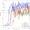 |
Fig. 1 Evolution of the maximum dust density with time for the monodisperse settling instability with four different resolutions (run1 to run4 in Table 1). Short horizontal lines on the left indicate averages between 60 and 100Ω−1 and the vertical dotted line indicates the settling time. |
4 Polydisperse simulations
After establishing the role of the DSI in forming high density dust structure in monodisperse simulations, we now turn to address how a distribution of dust sizes may change this picture. Our polydisperse simulations suite are summarised in Table 2. Here we fixed the dust properties to μ = 0.1 and stopping times, τs, between 0.001 and 0.1 following MRN distribution (Mathis et al. 1977), with τs and μ for each species chosen in the manner described in Section 2. We fixed the spatial resolution to 512 × 512 grid cells, and changed the number of dust species, n = 5, 10, and 20. Our first objective is to determine whether the DSI converges with the number of dust species modelled and, if so, how different the evolution is from that of monodisperse dust. To this end we used our monodisperse run10 with τs = 0.037 for comparison, as this presents the average stopping time for our polydisperse simulations. We note, however, that since the monodisperse DSI is not very sensitive to the stopping time, a very similar comparison could be made using the monodisperse simulation run3 (with τs = 0.1).
In Figure 5 we plot the time evolution of the maximum (total) dust density for the three polydisperse simulations and with n = 5, 10, and 20, as well as the monodisperse run10. The short horizontal lines on the left of the plot indicate averages between 60 and 100Ω−1. The averaged maximum dust density for poly10 is much closer to poly20 than poly5, indicating signs of convergence with the number of dust species. We caution, however, that we fixed the spatial resolution for this comparison, which may mean this result is not general as the spatial resolution may also affect the point at which we reach convergence with the number of species. One would need to vary both the spatial resolution and the number of dust species together for a more rigorous convergence study, which is beyond the scope of this work. We note that the maximum total dust density for poly20 is 4 times less than the monodisperse simulation with the same average τs, a reduction that is similar to that in the polydisperse SI (Matthijsse et al. 2025). In contrast to the SI, however, the saturation time for the DSI does not change much when going from mono- to polydisperse. This is crucial when assessing the viability of the polydisperse DSI, since the instability needs to develop within the settling time 1/(τsΩ).
4.1 Evolution of small dust: Monodisperse versus polydisperse
Krapp et al. (2020) looked at the non-linear evolution of the DSI for different stopping times through multiple independent monodisperse simulations and concluded that the DSI produces very little density structure at low τs and μ (see their Figure 3). In Figure 6 we present the dust density maps for three different species, τs = 0.00124, 0.01, and 0.08 (left to right) for the polydisperse run (top panels) and the three corresponding monodisperse runs (bottom panels) for a snapshot at t = 100Ω−1. These are the minimum, middle, and maximum stopping times for our poly5 simulation. While the DSI develops in the largest dust species to similar levels for both the mono- and polydisperse simulations, we can clearly see that for the intermediate and small dust species, the polydisperse treatment is able to capture much more density structure compared to the monodisperse simulations. We also observe a level of correlation between the structure formed in the different species in the polydisperse simulation.
Figure 7 shows the time evolution of the maximum dust density for the same three species as in Figure 6 for both the mono- and polydisperse simulations. Here we can appreciate more quantitatively the difference in evolution due to the polydisperse treatment. While the trigger time for the largest dust species is somewhat similar between poly- and mono-disperse simulations, we notice that the DSI is triggered earlier in the polydisperse simulation for the smaller dust species. We also see that, especially for the intermediate and small dust stopping times, the DSI results in larger dust density enhancements in the polydisperse simulations. Figure 7 indicates that, once the DSI is triggered for any dust species, its feedback on the gas causes the instability to occur in all other species. This is also hinted at by the apparent correlation observed in the structures formed by the DSI in the top panels in Figure 6.
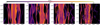 |
Fig. 2 Dust density for the monodisperse simulations at t = 80Ω−1. Panels show runs with different resolutions, increasing from left to right (run4 to run1). |
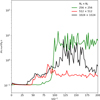 |
Fig. 3 Same as Figure 1 but with FARGO3D and excluding the highest resolution (run1, blue curve). We use the same limits for the y axis for an easier comparison, but we extend the x axis to t = 200Ω−1 |
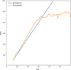 |
Fig. 4 Amplitude of perturbation as a function of time for the single mode perturbation simulation (orange) compared to the amplitude of the same mode computed from the analytical growth rate. |
Parameters for the polydisperse simulation suite.
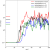 |
Fig. 5 Evolution of maximum (total) dust density with time for three polydisperse simulations with n = 5, 10, and 20, as well as the monodisperse run10. The short horizontal lines to the left indicate averages between 60 and 100Ω−1 and the vertical dotted line indicates the settling time for the monodisperse run10 (with a stopping time τs = 0.037 equivalent to the average stopping time of the polydisperse runs). |
4.2 Morphology
The correlation between dust structures at different τs shown in Figure 6 motivates us to further investigate the morphology of the polydisperse simulations. In Figure 8 we show the total dust density for the poly20 run at t = 90Ω−1, i.e. the sum of the densities from all 20 dust species. The long, thin filaments each correspond to overdensities in different dust species towards the high end of the τs range. Hence, the large-scale structure corresponds to multiple smaller structures from the different species. Intriguingly, each species seems to form similar-looking filaments to other species, but with a spatial offset.
In Figure 9 we plot the top 2% density for the highest six stopping times (coloured open curves) as well as the top 5% total density of the sum of all 20 species (filled black curve), for the same snapshot shown in Figure 8. We notice how different dust species form different filaments and are coherent but offset from each other. The filled black contours, representing the highest total dust density regions, often coincide with separate filaments from individual species. While the structures formed in different dust species are clearly correlated, they tend to be spatially separated. This means that, while large-scale structure will contain contributions from dust with different stopping times, at small scales dust interactions are mostly monodisperse, involving dust particles with similar stopping times.
A closer inspection of Figure 9 shows the tendency for the size-segregated structures to form a τs gradient. The direction of the gradient varies with the details of the flow. The open contours in Figure 9 line up right to left in order of decreasing τs in the top multi-species filament, and the opposite direction in the middle filament. Examining the over-density in the sum of all species (filled black contours), we notice that they are more likely to overlap with lower τs contours (cyan and violet) than high τs (red and blue). The trend does not continue to even lower τs; we only show the highest 6 out of 20 τs species to reduce clutter, but Figures 6 and 7 show that low τs dust is less efficient in clumping.
The fact that the highest total density regions are more likely to overlap with structures formed by species that are not the high end of the τs range indicates that there might be a peak in the dust size distribution resulting from the DSI. This is similar to the peak reported in the polydisperse SI, which is also caused by the spatial segregation of dust with different sizes and the τs gradient that results from it (Matthijsse et al. 2025). We test this implication in Figure 10, in which we plot the time evolution of the dust size distribution as a function of τs for the top 10% in dust density, normalised by the initial MRN distribution. While there is a considerable scatter, we can see there is a tendency for the maximum of the distribution to occur at τs less than the maximum. Comparing Figure 10 to Figure 6 in Matthijsse et al. (2025), we see that the SI produces a much better defined peak in the size distribution, with considerably less scatter, than the DSI. This may be due to the fact that the DSI tends to produce larger filaments stretching throughout the simulation box, and thus the statistics of the size distribution are heavily influenced by the evolution of each filament, whereas the SI tends to produce numerous but smaller structures, and therefore the size distribution is less sensitive to evolution of each structure.
5 Discussion and conclusion
The DSI has been shown to have analytical growth rates in the linear regime orders of magnitude higher than the SI and independent of the stopping time (Squire & Hopkins 2018b). However, for the DSI to play an important role in planetesimal formation, it needs to reach maximum dust densities in the non-linear regime comparable to the ones of the SI, and, importantly, form these high-density structures faster than the settling time, which is seen as the more important barrier (Krapp et al. 2020). In our monodisperse simulations, our results show a trend suggesting that both criteria could be met at higher (currently unprobed) spatial resolutions, as a higher resolution both increases the maximum dust density and shortens the time it takes for the DSI to form structure. This is a main difference between the SI and DSI: while spatial resolution increases the maximum dust density, it does not shorten the saturation time (Matthijsse et al. 2025). This is likely due to the fact that linear growth in the DSI is dominated by the double resonance2, which increases indefinitely with wavenumber. We note, however, that the ability of the DSI to outpace the settling time is affected by the amplitude of the initial seed perturbations in our simulations. Regarding the maximum dust density attained by the DSI, diffusion (which was not taken into account in this paper) will set a limit on the maximum wavenumber that contributes to the DSI, and spatial convergence will be reached. Much like the SI (Chen & Lin 2020; McNally et al. 2021), the level of dust diffusion and gas viscosity is also likely to limit clumping due to the DSI, as is shown for the linear regime in Figure 10 in Paardekooper & Aly (2025b).
In this paper we attempted two types of comparisons between mono- and polydisperse DSI simulations. First, we compared polydisperse simulations with 5, 10, and 20 dust species (poly5, poly10, and poly20) to a single monodisperse simulation (run10) with a dust-to-gas ratio, μ, equal to that of the total combined μ across all dust species in each polydisperse run, and a monodisperse stopping time equal to the average stopping time of the polydisperse runs (Figure 5). This comparison showed that, while the maximum dust density obtained for the polydisperse runs is less than the monodisperse one by a factor of a few (similar to the SI, see Matthijsse et al. 2025), the saturation time of mono- and polydisperse runs is very similar (unlike the SI trends). This is somewhat expected from the linear analysis in Paardekooper & Aly (2025b), where it is shown that the size distribution has a much more significant negative effect for the SI than the DSI. Figure 5 also showed that the polydisperse simulations seem to approach convergence with the number of dust species at about n = 10 (with the caveat that this test was only performed at a fixed spatial resolution).
Second, we compared a single polydisperse simulation (poly5) with five different monodisperse runs (run5 to run9), each with μ and τs equal to a corresponding species in the poly5 run. This comparison showed that the polydisperse treatment results in a significantly different dust evolution. Structure forms for all τs in our size distribution in polydisperse simulations, whereas only high τs dust forms structure in corresponding monodisperse ones (Figures 6 and 7).
The spatial distribution of the highest density regions shows that the polydisperse DSI exhibits a filamentary structure. Dust with different sizes tends to form adjacent thin filaments, which seem to be ordered, with the largest dust forming filaments at the edge of the bigger structure (Figure 9). The highest overall density regions tend to disfavour these edge filaments, leading to a dust size distribution that does not monotonically increase with dust size (Figure 10). Matthijsse et al. (2025) recently reported a similar trend for the polydisperse SI, with the main difference being that the SI forms several smaller filaments, whereas the DSI tends to form one bigger dust structure in spanning the computational domain.
Our results indicate that the polydisperse DSI shows potential in forming clumps and is likely important for planetesimal formation. In cases in which the DSI does not form clumps with high-enough densities to trigger gravitational collapse (on a timescale shorter than the settling time), it can still play a role in creating overdensities that facilitate the onset of the SI or the closely related vertically shearing SI (VSSI, Lin 2021). This latter scenario is particularly plausible as the DSI operates in the upper disc layers, whereas the SI and VSSI operate in the midplane as the dust settles, creating a natural ordering whereby the DSI leads to other drag instabilities, rather than compete with them.
We note that an important caveat in this work is the local treatment of stratification, similar to Krapp et al. (2019), represented by the terms proportional to z0 in Eqs. (2) and (6). Dust settling is inherently a stratified process and the DSI may manifest very differently if we take into account the vertical gas pressure gradient in a more realistic way. Moreover, this approximate treatment of vertical gravity obliged us to use a simulation box with a small vertical extent (otherwise it becomes harder to justify the unstratified assumption), which may underestimate the resulting maximum dust density. We also had to add an effective acceleration to the gas to account for the vertical backreaction from the settling dust, which is strictly speaking only in equilibrium in the initial conditions and may inaccurately affect the evolution of both gas and dust. A more faithful assessment of the role of the DSI in planet formation requires a self-consistent stratified approach. Moreover, in such a selfconsistent stratified vertically global set-up, one would expect other instabilities to take place. These would include pure hydro instabilities such as the vertical shear instability (VSI, Urpin & Brandenburg 1998; Nelson et al. 2013) and the Kelvin-Helmholtz (KH) instability (Sekiya 1998; Johansen et al. 2006), as well as drag instabilities such as VSSI and the classical SI near the midplane or in regions where the dust-to-gas ratio approaches unity (Schäfer et al. 2025). The interplay between these different instabilities may fundamentally change the nature of the DSI and its role in forming dust clumps in a stratified, vertically global set-up.
We also note that even within the unstratified and vertically local treatment we adopted here, we have assumed a strictly isothermal equation of state and thus neglected the effects of cooling and buoyancy. A more careful treatment of the thermodynamics would implicitly take into account vertical gradients and shear, which is likely to affect both the VSI and DSI. Lehmann & Lin (2023) performed a linear stability analysis of a local unstratified shearing box but included the effects of buoyancy using the Boussinesq approximation (Latter & Papaloizou 2017) and showed that in the linear regime vertical buoyancy greatly stabilises the DSI (apart from a narrow band in k space around the resonances). However, they also reported a new instability, the dust settling shearing instability (DSSI), which can be thought of as a combination of the VSI and DSI when both dust-settling and vertical shear in the gas are accounted for, with growth rates in the linear regime that may exceed either of the classical versions of the instabilities. The interplay between these instabilities, and the way they manifest in the non-linear regime, warrants future investigation.
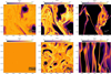 |
Fig. 6 Dust density at t = 100Ω−1 for three different species, τs = 0.00124, 0.01, and 0.08 (left to right) for the polydisperse run poly5 (top panels) and the three corresponding monodisperse runs (bottom panels). Note that the colour bar limits are fixed for the same τs (top and bottom panels), but the maximum value increases by an order of magnitude as τs increases (left to right) |
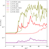 |
Fig. 7 Time evolution of the maximum dust density for the same three species as in Figure 6 for the monodisperse (runs 5, 7, and 9) and poly5 simulations. |
 |
Fig. 8 Total dust density for the poly20 run at t = 90Ω−1. |
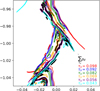 |
Fig. 9 Coloured open curves represent contours of the top 2% density for the highest six stopping times (see figure legend) for the same snapshot shown in Figure 8. The filled black curve represents the top 5% total density of the sum of all 20 species. |
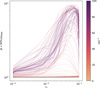 |
Fig. 10 Evolution of the dust size distribution as a function of τs for the top 10% in dust density, normalised by the initial MRN distribution. |
Data availability
The data and scripts used to produce the figures in this paper are available at: https://doi.org/10.4121/f45864ae-5e02-41e9-8a2f-f73a2d7086d7
Acknowledgements
We thank the anonymous referee for a detailed report and helpful suggestions. We thank Jip Matthijsse for fruitful discussions. This project has received funding from the European Research Council (ERC) under the European Union Horizon Europe programme (grant agreement No 101054502). The authors acknowledge the use of computational resources of the Delft-Blue supercomputer, provided by Delft High Performance Computing Centre (https://www.tudelft.nl/dhpc).
Appendix A Settling instability with FARGO3D
Our attempts to simulate the DSI with FARGO3D presented in Figure 3 show a decrease in the dust ability to clump with increasing resolution from run4 to run3 (though it seems the trend is reversed increasing the resolution further from run3 to run2), which the opposite of what we expect. We attributed this to numerical artifacts that develop in the gas in the shape of stripes. These have been reported before in the case of the SI (Benítez-Llambay et al. 2019; Matthijsse et al. 2025), in which case they have only been noticed in the gas and did not seem to affect the dust evolution.
Here we take a closer look at this phenomenon. We plot the gas and dust density fields for a snapshot at t = 100Ω−1 in Figure A.1 for run4, run3, and run2 (top to bottom). We can see clear stripes showing in the gas density for the higher resolution runs (run4 at the top only shows fainter ripple). While the stripes do not show in the dust density field, they seem to have a strong effect on the clumping, as it greatly decreases for the higher resolution runs where the gas stripes are more evident (note that while the color bar limits are different for gas and dust, they are kept the same for the different resolutions for an easier comparison). In Figure A.2 we show the radial velocity fields for both gas and dust for the same snapshot. Here we see the stripes in both gas and dust for the higher resolution runs, which strongly suggests that the negative effect on clumping at higher resolution is indeed caused by these numerical artifacts. Figures A.1 and A.2 also indicate a slight reduction of the strength of these stripes going from run3 to run2, which would be expected from the time series of the maximum dust density in Figure 3.
Krapp et al. (2020) simulated the monodisperse DSI with varying physical numerical parameters using FARGO3D. Their simulation corresponding to our runs 1 through 4 (i.e. τs = 0.1 and μ = 0.1) used a box with dimensions Lx = 0.1z0 and Lx = 0.5z0 with 1024 × 2560 grid cells and reported a time-average of the maximum dust density 22ρg. Note that this set-up has higher resolution in the horizontal than in the vertical direction. We repeat this set-up for a more consistent comparison. We also simulate the same box with higher vertical resolution with 1024 × 5120 grid cells to see whether the same trend observed in runs 2 to 4 applies here. We show a snapshot of the dust density at t = 80Ω−1 for both simulations in Figure A.3. The lower resolution run (left) is consistent with that reported in Krapp et al. (2020). We notice that dust clumps more efficiently in the lower resolution run, with a maximum dust density of 23.3ρg, similar to that reported in Krapp et al. (2020). The higher resolution run (right) shows a much less efficient clumping, with a maximum dust density almost an order of magnitude lower.
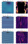 |
Fig. A.1 Gas (left) and dust (right) densities for a snapshot at t = 100Ω−1 for run4, run3, and run2 (top to bottom). Note the visible stripes in the gas, while for the dust clumping is noticeably stronger for the lowest resolution |
 |
Fig. A.2 Same as Figure A.1 but for radial velocity. Here we can see the numerical stripes for run3 and run2 in both gas and dust |
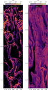 |
Fig. A.3 Dust density at t = 80Ω−1 for a more vertically extended shearing box. Left: 1024 × 2560 grid cells, consistent with Krapp et al. (2020). Right: 1024 × 5120 grid cells |
References
- Benítez-Llambay, P., & Masset, F. S. 2016, ApJS, 223, 11 [Google Scholar]
- Benítez-Llambay, P., Krapp, L., & Pessah, M. E. 2019, ApJS, 241, 25 [Google Scholar]
- Birnstiel, T., Ormel, C. W., & Dullemond, C. P. 2011, A&A, 525, A11 [NASA ADS] [CrossRef] [EDP Sciences] [Google Scholar]
- Blum, J., & Wurm, G. 2008, ARA&A, 46, 21 [Google Scholar]
- Chen, K., & Lin, M.-K. 2020, ApJ, 891, 132 [Google Scholar]
- Chiang, E., & Youdin, A. N. 2010, Ann. Rev. Earth Planet. Sci., 38, 493 [Google Scholar]
- Delft High Performance Computing Centre (DHPC) 2024, DelftBlue Supercomputer (Phase 2), https://www.tudelft.nl/dhpc/ark:/44463/DelftBluePhase2 [Google Scholar]
- Epstein, P. S. 1924, Phys. Rev., 23, 710 [Google Scholar]
- Goldreich, P., & Lynden-Bell, D. 1965, MNRAS, 130, 125 [Google Scholar]
- Goldreich, P., & Ward, W. R. 1973, ApJ, 183, 1051 [Google Scholar]
- Hawley, J. F., Gammie, C. F., & Balbus, S. A. 1995, ApJ, 440, 742 [Google Scholar]
- Huang, P., & Bai, X.-N. 2022, ApJS, 262, 11 [NASA ADS] [CrossRef] [Google Scholar]
- Johansen, A., & Youdin, A. 2007, ApJ, 662, 627 [Google Scholar]
- Johansen, A., Henning, T., & Klahr, H. 2006, ApJ, 643, 1219 [NASA ADS] [CrossRef] [Google Scholar]
- Johansen, A., Oishi, J. S., Mac Low, M.-M., et al. 2007, Nature, 448, 1022 [Google Scholar]
- Krapp, L., Benítez-Llambay, P., Gressel, O., & Pessah, M. E. 2019, ApJ, 878, L30 [Google Scholar]
- Krapp, L., Youdin, A. N., Kratter, K. M., & Benítez-Llambay, P. 2020, MNRAS, 497, 2715 [NASA ADS] [CrossRef] [Google Scholar]
- Latter, H. N., & Papaloizou, J. 2017, MNRAS, 472, 1432 [CrossRef] [Google Scholar]
- Lehmann, M., & Lin, M.-K. 2023, MNRAS, 522, 5892 [CrossRef] [Google Scholar]
- Lesur, G. R. J., Baghdadi, S., Wafflard-Fernandez, G., et al. 2023, A&A, 677, A9 [NASA ADS] [CrossRef] [EDP Sciences] [Google Scholar]
- Li, R., & Youdin, A. N. 2021, ApJ, 919, 107 [NASA ADS] [CrossRef] [Google Scholar]
- Lin, M.-K. 2021, ApJ, 907, 64 [Google Scholar]
- Magnan, N., Heinemann, T., & Latter, H. N. 2024a, MNRAS, 529, 688 [NASA ADS] [CrossRef] [Google Scholar]
- Magnan, N., Heinemann, T., & Latter, H. N. 2024b, MNRAS [arXiv:2408.07441] [Google Scholar]
- Mathis, J. S., Rumpl, W., & Nordsieck, K. H. 1977, ApJ, 217, 425 [Google Scholar]
- Matthijsse, J., Aly, H., & Paardekooper, S.-J. 2025, A&A, 695, A158 [NASA ADS] [CrossRef] [EDP Sciences] [Google Scholar]
- McNally, C. P., Lovascio, F., & Paardekooper, S.-J. 2021, MNRAS, 502, 1469 [NASA ADS] [CrossRef] [Google Scholar]
- Nakagawa, Y., Sekiya, M., & Hayashi, C. 1986, Icarus, 67, 375 [Google Scholar]
- Nelson, R. P., Gressel, O., & Umurhan, O. M. 2013, MNRAS, 435, 2610 [Google Scholar]
- Paardekooper, S.-J., & Aly, H. 2025a, A&A, 696, A53 [NASA ADS] [CrossRef] [EDP Sciences] [Google Scholar]
- Paardekooper, S.-J., & Aly, H. 2025b, A&A, 697, A40 [NASA ADS] [CrossRef] [EDP Sciences] [Google Scholar]
- Paardekooper, S.-J., McNally, C. P., & Lovascio, F. 2020, MNRAS, 499, 4223 [CrossRef] [Google Scholar]
- Paardekooper, S.-J., McNally, C. P., & Lovascio, F. 2021, MNRAS, 502, 1579 [NASA ADS] [CrossRef] [Google Scholar]
- Safronov, V. S. 1969, Evoliutsiia doplanetnogo oblaka. (.) [Google Scholar]
- Schäfer, U., Johansen, A., & Flock, M. 2025, A&A, 694, A57 [NASA ADS] [CrossRef] [EDP Sciences] [Google Scholar]
- Sekiya, M. 1998, Icarus, 133, 298 [CrossRef] [Google Scholar]
- Squire, J., & Hopkins, P. F. 2018a, MNRAS, 477, 5011 [Google Scholar]
- Squire, J., & Hopkins, P. F. 2018b, ApJ, 856, L15 [NASA ADS] [CrossRef] [Google Scholar]
- Toro, E. F., Spruce, M., & Speares, W. 1994, Shock Waves, 4, 25 [Google Scholar]
- Urpin, V., & Brandenburg, A. 1998, MNRAS, 294, 399 [Google Scholar]
- Weidenschilling, S. J. 1977, MNRAS, 180, 57 [Google Scholar]
- Weidenschilling, S. J. 1980, Icarus, 44, 172 [NASA ADS] [CrossRef] [Google Scholar]
- Yang, C.-C., & Zhu, Z. 2021, MNRAS, 508, 5538 [NASA ADS] [CrossRef] [Google Scholar]
- Youdin, A. N., & Goodman, J. 2005, ApJ, 620, 459 [Google Scholar]
- Youdin, A., & Johansen, A. 2007, ApJ, 662, 613 [Google Scholar]
- Zhuravlev, V. V. 2019, MNRAS, 489, 3850 [NASA ADS] [Google Scholar]
Note that our definition of the pressure support parameter, η, is consistent with Paardekooper et al. (2020, 2021); Matthijsse et al. (2025), but is different from the definition widely used in the literature (Youdin & Goodman 2005), such that η = r0Ω2ηYG. This definition of η is dimensional by choice, and results in a length scale, η/Ω2, independent of r0, which does not play a role in a local framework. The timescale is defined by Ω−1.
At a high radial wavenumber, kx, the growth rate in the linear regime increases without bound with the wavenumber (Squire & Hopkins 2018a). This is called the double resonance angle as both the SI and DSI unstable branches merge (in wavenumber space), where the criterion k · Δv = 0 is met (with v being the drift velocity).
All Tables
All Figures
|
Fig. 1 Evolution of the maximum dust density with time for the monodisperse settling instability with four different resolutions (run1 to run4 in Table 1). Short horizontal lines on the left indicate averages between 60 and 100Ω−1 and the vertical dotted line indicates the settling time. |
| In the text | |
|
Fig. 2 Dust density for the monodisperse simulations at t = 80Ω−1. Panels show runs with different resolutions, increasing from left to right (run4 to run1). |
| In the text | |
|
Fig. 3 Same as Figure 1 but with FARGO3D and excluding the highest resolution (run1, blue curve). We use the same limits for the y axis for an easier comparison, but we extend the x axis to t = 200Ω−1 |
| In the text | |
|
Fig. 4 Amplitude of perturbation as a function of time for the single mode perturbation simulation (orange) compared to the amplitude of the same mode computed from the analytical growth rate. |
| In the text | |
|
Fig. 5 Evolution of maximum (total) dust density with time for three polydisperse simulations with n = 5, 10, and 20, as well as the monodisperse run10. The short horizontal lines to the left indicate averages between 60 and 100Ω−1 and the vertical dotted line indicates the settling time for the monodisperse run10 (with a stopping time τs = 0.037 equivalent to the average stopping time of the polydisperse runs). |
| In the text | |
|
Fig. 6 Dust density at t = 100Ω−1 for three different species, τs = 0.00124, 0.01, and 0.08 (left to right) for the polydisperse run poly5 (top panels) and the three corresponding monodisperse runs (bottom panels). Note that the colour bar limits are fixed for the same τs (top and bottom panels), but the maximum value increases by an order of magnitude as τs increases (left to right) |
| In the text | |
|
Fig. 7 Time evolution of the maximum dust density for the same three species as in Figure 6 for the monodisperse (runs 5, 7, and 9) and poly5 simulations. |
| In the text | |
|
Fig. 8 Total dust density for the poly20 run at t = 90Ω−1. |
| In the text | |
|
Fig. 9 Coloured open curves represent contours of the top 2% density for the highest six stopping times (see figure legend) for the same snapshot shown in Figure 8. The filled black curve represents the top 5% total density of the sum of all 20 species. |
| In the text | |
|
Fig. 10 Evolution of the dust size distribution as a function of τs for the top 10% in dust density, normalised by the initial MRN distribution. |
| In the text | |
|
Fig. A.1 Gas (left) and dust (right) densities for a snapshot at t = 100Ω−1 for run4, run3, and run2 (top to bottom). Note the visible stripes in the gas, while for the dust clumping is noticeably stronger for the lowest resolution |
| In the text | |
|
Fig. A.2 Same as Figure A.1 but for radial velocity. Here we can see the numerical stripes for run3 and run2 in both gas and dust |
| In the text | |
|
Fig. A.3 Dust density at t = 80Ω−1 for a more vertically extended shearing box. Left: 1024 × 2560 grid cells, consistent with Krapp et al. (2020). Right: 1024 × 5120 grid cells |
| In the text | |
Current usage metrics show cumulative count of Article Views (full-text article views including HTML views, PDF and ePub downloads, according to the available data) and Abstracts Views on Vision4Press platform.
Data correspond to usage on the plateform after 2015. The current usage metrics is available 48-96 hours after online publication and is updated daily on week days.
Initial download of the metrics may take a while.