| Issue |
A&A
Volume 701, September 2025
|
|
|---|---|---|
| Article Number | A281 | |
| Number of page(s) | 12 | |
| Section | Interstellar and circumstellar matter | |
| DOI | https://doi.org/10.1051/0004-6361/202554534 | |
| Published online | 25 September 2025 | |
Observation of new interstellar clouds in the Libra constellation inside the Local Bubble
1
Department of Astronomy, ELTE Eötvös Loránd University, 1117 Budapest, Pázmány P. s. 1/A, Hungary
2
University of Debrecen, Institute of Physics, Debrecen, Hungary
3
Astropolarimetry Research Group, Office of Supported Research Groups, Hungarian Research Network, 1052 Budapest, Piarista utca 4, Hungary
4
Environmental Optics Laboratory, Department of Biological Physics, ELTE Eötvös Loránd University, 1117 Budapest, Pázmány P. s. 1/A, Hungary
5
Fornax 2002 Ltd., 2119 Pécel, Ady Endre utca 1, Hungary
★★ Corresponding author: This email address is being protected from spambots. You need JavaScript enabled to view it.
Received:
14
March
2025
Accepted:
22
July
2025
Abstract
Context. The structure of the interstellar medium of our immediate Galactic environment has typically been studied by extinction, line emission, and absorption measurements. Interstellar clouds with moderate extinction (0.3 < AG < 1), however, may also appear as reflection nebulae in scattered light. Nearby translucent clouds may be detected by their cloud shine even inside the Local Bubble.
Aims. We explore a so far less studied area at high Galactic latitude in a search for translucent clouds inside the Local Bubble.
Methods. We mapped the sky in the visible spectral range on 21 July 2023 on the Namibian Khomas Highland with our telescope, which has a wide field of view. Optical imaging combined with multi-wavelength data helped us to localize clouds. We used Gaia DR3 data to estimate their distances and then derived their physical parameters.
Results. We detected a pattern of elongated reflection nebulae in the Libra constellation at high Galactic latitudes (l = 332°, b = 36°). The stripes of this new interstellar cloud are roughly parallel to the Galactic plane and are associated with similar structures seen in H I 21 cm maps. We identified four cloud layers: (i) The nearest component with an extinction of AG ≤ 0.2 is closer than 50 pc. (ii) The second component with an extinction of AG 0.5 has an estimated distance of 60 pc. (iii) The third component lies at 75 pc with a similar extinction. (iv) The fourth component with an extinction of AG > 1.5 and an estimated distance of 135 pc may correspond to the wall of the Local Bubble (or Local Chimney), while the former components are inside of this wall. We named these clouds the Zebra nebula system because they have strong stripes. The cloud with the highest extinction in the centre of the region we studied is called the Zebra1 nebula. The size of this interstellar cloud is 6.5 pc × 1.6 pc, and it consists of mostly neutral atomic hydrogen, but small dense parts of the cloud may be molecular. Its total mass is 70M⊙ × (d/[60] pc)2. The Zebra1 nebula is surrounded by other less opaque clouds with similar distances. They are all located inside the Local Bubble.
Conclusions. Wide-field optical imaging is capable of locating nearby high-latitude interstellar clouds. Apparently, there are still clouds to discover inside the Local Bubble (or Local Chimney).
Key words: catalogs / surveys / ISM: bubbles / ISM: clouds / ISM: molecules
Both first two authors contributed equally to this article.
© The Authors 2025
 Open Access article, published by EDP Sciences, under the terms of the Creative Commons Attribution License (https://creativecommons.org/licenses/by/4.0), which permits unrestricted use, distribution, and reproduction in any medium, provided the original work is properly cited.
This article is published in open access under the Subscribe to Open model. This email address is being protected from spambots. You need JavaScript enabled to view it. to support open access publication.
1 Introduction
Models of the distribution of cold interstellar medium around the Solar System pictured an evacuated cavity, the Local Bubble (LB), that is surrounded by a shell of swept-up gas and dust, as shown by Cox & Reynolds (1987) and Welsh & Shelton (2009), for example. Several authors recently modeled the 3D structure of the LB and the nearby interstellar medium in general based on stellar photometric data from the data releases Gaia DR2 (Gaia Collaboration 2018) and DR3 (Gaia Collaboration 2021) and other all-sky data, such as Lallement et al. (2019) Leike et al. (2020) Linsky & Redfield (2021) Zucker et al. (2022). Edenhofer et al. (2024) also released a 3D dust map with an angular resolution of up to 14′ for the 69 pc to 1250 pc distance range from the Solar System, while Dharmawardena et al. (2024) recently extended the integrated extinction mapping to 2.8 kpc with a sampling of l, b, d = 1° × 1° × 1.7 pc. Rybarczyk et al. (2024) used H I spectral and extinction data to identify cold neutral medium (CNM) structures that may be associated with the LB wall. The surface of the LB with an internal width of ~200 pc is not closed, but extends perpendicular to the Galactic plane, 250– 300 pc above and below, forming the Local Chimney (O’Neill et al. 2024). Breitschwerdt et al. (2016) interpreted the LB as a structure that was created by a supernova explosion, which may also have triggered star formation in all the nearest star-forming regions, as shown by Zucker et al. (2022), for example. The cavity is filled with extremely low-density hot plasma (Sanders et al. 1977), but there are also warm translucent clouds, such as the Local Interstellar Cloud (LIC) and its neighbors within 15 pc (see Redfield & Linsky 2008; Frisch et al. 2011, Redfield & Linsky 2015), and even molecular clouds such as MBM33 and MBM35 with distances shorter than 100 pc (Zucker et al. 2019).
Translucent nearby dark clouds may be seen in forward-directed scattering, as shown by Mattila (1970) and Mattila et al. (2018), for instance. This alternative way of discovery was applied in our wide-field observations to locate new clouds in Libra.
2 Data and methods
2.1 Optical observations
Our photographic observation was performed in the Isabis Astro Lodge (16°28′55″ East, 23°26′19″ South, altitude ~1800 m) on the Namibian Khomas Highland under a cloudless and aerosol-free sky, far from city lights (the nearest town was over 70 km away). Our telescope with a wide field of view of 15°26 (horizontal) ×10°.18 (vertical) was moved by a motor-driven German Equatorial Fornax 51 Telescope Mount (Fornax Ltd., Pécel, Hungary) and was controlled with the telescope drive master (MDA-Invent Kft., Érd, Hungary) tracking system with increased precision. Our camera was a full-frame (24 mm × 36 mm) back-illuminated astrocamera with a cooled monochromatic CMOS sensor (Moravian C3-61000EC Pro, Moravian Instrument, Zlin, Czech Republic). The Fornax 51 Telescope Mount was guided by an FS-2 controller and a SkyTools 4 software. The telescope had a Sigma 135 mm/F1.8 Art telephoto lens.
Figure 1 shows our measurement site and telescope instruments in the Isabis Astro Lodge of the Namibian Khomas Highland. The images were taken on 21 and 23 July 2023 with an exposure time of 600 s, centered at around (l = 332°, b = 36°). The quality of the nocturnal sky was 21.85-21.95 magnitude/arcsec2, which corresponds to level 1 in the Bortle scale (Bortle 2001). A repeated measurement in roughly the same sky window (with a slight RA offset) two days later was performed to confirm the detection of an earlier uncataloged formation in the Libra constellation.
The photographs were controlled and processed using the MaximDL software. The images were calibrated with bias, dark, and flat frames (including flat darks). Further technical details can be found in Slíz-Balogh et al. (2024).
No filters were used for the images, so that the bandwidth and spectral distribution of the image were determined solely by the inherent characteristics of the Moravian C3-61000EC Pro camera Sony IMX455 full-frame monochrome sensor. The relative quantum efficiency spectrum of the sensor is shown in Fig. 2.
Our images of the region are presented in Fig. 3. They each cover a size of 15°26 × 10°.18 in the sky area. For example, image (A) is centered at l = 332°, b = 36° and shows 14h06m17s ≤ RA ≤ 15h07m17s, -21°33′50″ ≤ Dec ≤ -11°23′2″.
2.2 Planck all-sky extinction data
The distribution of dust that may cause the observed cloud shine pattern in the region was studied using the extinction data of Planck Collaboration Int. XXIX (2016). Their 5′ spatial resolution full-sky dust map is based on fitting Planck, IRAS, and WISE data, and it was calibrated with interstellar extinction values observed for QSOs. We downloaded AV_RQ (V band) visual extinction data from the Planck Legacy Archive1 server. A 15° × 15° region is shown in Fig. 4.
2.3 HI4PI survey H I 21 cm data
In order to identify the velocity-coherent interstellar clouds that cause the detected cloud shine, H I 21 cm data of the region were also investigated. This part of the sky was observed with the Parkes 64m radio telescope (McClure-Griffiths et al. 2009) with a beam size of 16′.2 in the GASS survey (Kalberla & Haud 2015), and the processed data are stored in the HI4PI database (HI4PI Collaboration 2016). We took individual spectra and channel maps from the HI4PI data server of the H I survey server of the Argelander-Institut für Astronomie2. A sample H I 21 cm spectrum is shown in Fig. 5.
We drew a map of the hydrogen column density using the Aladin Sky Server Bonnarel et al. (2000) based on the HI4PI full sky H I survey by HI4PI Collaboration (2016) to locate clouds of neutral hydrogen. The total hydrogen column density distribution of the region is shown in Fig. 6.
Local hydrogen column density peaks were defined by the N(H) = 8 × 1020 cm-2 contour. We then downloaded for each of them ON and two OFF H I 21 cm spectra. The ON-spectra (average of two OFF) were then calculated to correct for the immediate foreground and background. In this way, the peculiar velocity of each N (H) peak was derived.
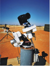 |
Fig. 1 Measurement site of our observations at the Isabis Astro Lodge in the Namibian Khomas Highland with our portable telescope. Photo by Pál Sári. |
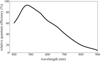 |
Fig. 2 Relative quantum efficiency of the CMOS camera sensor of our polarimetric telescope as a function of wavelength (nm). |
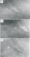 |
Fig. 3 Photometric images of the region in the constellation Libra. The size of the images is 15°.26 × 10°.18. The brightest star in the images is the spectroscopic binary alf02 Lib at RA = 14h50m52.71s Dec = -16°02′30″.4. Top: picture center at RA = 14h36m47s, Dec = -16°28′26″) taken on 21 July 2023 at 18:24:57 UT. Middle: picture center at RA = 14h56m47s, Dec = -16°28′26″ taken on 21 July 2023 at 18:44:58. Bottom: picture center at RA = 14h41m47s, Dec = -16°28′26″ taken on 23 July 2023 at 18:58:54 UT. Photos by Judit Slíz-Balogh and Attila Mádai. |
 |
Fig. 4 AV_RQ (V band) visual extinction map from the Planck Legacy Archive centered on RA = 14h40m, Dec = -16°. The contours are drawn at 0.3, 0.38, 0.46, 0.54, 0.62, and 0.7 magnitudes. The Zebra nebula is shown roughly in the middle. An equatorial coordinate grid is overlaid. |
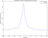 |
Fig. 5 Sample GASS (Kalberla & Haud 2015) H I 21 cm spectrum from the HI4PI archive at l = 336° 137, b = 40°.257 RA = 14h34m27.4s, Dec = -15° 52′48″. |
2.4 Gaia data and cloud layer distances
We investigated the extinction of stars within the observed field. Line-of-sight interstellar clouds increase the AG extinction of the stars behind it, which causes a break point in the extinction versus distance diagram of stars along the line of sight. We determined the cloud layer distance based on locating these break points (see e.g., Maheswar et al. (2010) and Straižys et al. (2018).
As the first step, we selected Gaia DR3 stars on the basis of AG extinction and d distance as AG ≥ 0.01 and d < 180 pc from the same sky window as in Fig. 3(A). In total, 3822 stars met both criteria. Figure 7 depicts the AG extinction of these stars as a function of distance.
We zoom-in on smaller distances in Fig. 7 in order to explore the nearby layers of the interstellar medium. Figure 8 shows the full distance-extinction distribution for the 0 pc < d < 100 pc.
The distance-dependent extinction of the diffuse Galactic dust can be estimated using the Parenago (1945) law, which we explain and provide current revisions for in Appendix A. This curve would describe the crowd of points in Figs. 7 and 8, with the lowest extinctions. In order to show the data of these stars better, we zoom-in on AG < 0.1 and 0 pc < d < 100 pc in Fig. 9. The data points of stars at off-cloud sight-lines would follow this curve and present a sort of baseline (Yan et al. 2019). This baseline is especially important in a search for the nearest cloud layers. We used moving average and curve fitting in various subregions of the AG versus distance diagrams to locate break points, as shown by Maheswar et al. (2010), for example.
By investigating the upper and lower limits given for the stellar distances and extinctions in Gaia DR3, we gauged the accuracy of the distance and extinction values. The distance error bars are typically smaller than 1 pc, and the AG error bars are typically smaller than 0.02 below a distance of 100 pc.
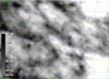 |
Fig. 6 Total hydrogen column density distribution based on the full sky H I survey by HI4PI Collaboration (2016). The boundary of the optical frame is overlaid (yellow). Gaia stars with a G-band extinction of AG ≥ 0.3 Gaia at a distance of d ≤ 80 pc are overplotted (filled red circles). |
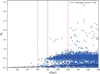 |
Fig. 7 Distance vs extinction diagram based on 3822 stars in the Gaia DR3 taken from the sky window (14h06m 17s ≤ RA ≤ 15h07m 17s, -21°33′50″≤ DE ≤ -11°23′2″), as Fig. 3(A). The vertical red lines mark break points at about 60, 80, and 120 pc. |
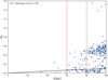 |
Fig. 8 Distance vs. extinction diagram based on the Gaia DR3 taken from the sky window of Fig. 3(A), but limited to distances d < 100 pc. The vertical red lines mark the break points at about 60 and 80 pc. |
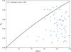 |
Fig. 9 Distance vs. extinction diagram based on the Gaia DR3 taken from the sky window of Fig. 3(A), but limited to distances d < 100 pc and extinctions AG < 0.1. |
2.5 Identifying individual interstellar clouds
Although we studied a high-latitude region, projection effects might mimic structures. In order to identify interstellar clouds, we searched for velocity-coherent structures using the H I 21 cm survey data in the directions of the object candidates of the multiwavelength sky surface brightness data. We determined the cloud borders following the contours in the H I 21 cm channel maps.
We then repeated the Gaia extinction-distance analysis for each of them. As an example, Fig. 10 shows the distribution of stars and the derived diagram for the central cloud structure.
3 Results
3.1 ISM layers that cause the extinction
There is a moderate extinction in the studied region. The minimum and average values of the Planck-based extinction (Planck Collaboration Int. XXIX 2016) in the 150 square degree region are AV,min = 0.17 and  , respectively. When stars with AG < 0.01 are excluded, the distribution of the Gaia DR3 AG extinction values shows two peaks with midpoints at AG = 0.1 and AG = 0.5 mag (see Fig. 11). There are further local maxima at AG = 1, AG = 1.5 and AG = 2. The latter two are not visible in the truncated histogram.
Based on Figs. 4 and 6, the studied region is dominated by structures of moderate extinction and column density with AV > 0.4 and N(H) > 7 × 20cm-2. Following Jordi et al. (2010), the conversion factor between V and G band extinction is in the range of
 (1)
(1)
We note that using relation (1) and Güver & Özel (2009) on the AV to N (H) ratio, we calculate it as
![Mathematical equation: N(\mathrm{H})_\mathrm{ext}/[\mathrm{cm}^{-2}]=2.2\times 10^{21}A_\mathrm{V}\approx 2.5\times 10^{21}A_\mathrm{G}.](/articles/aa/full_html/2025/09/aa54534-25/aa54534-25-eq3.png) (2)
(2)
Considering this and also Figs. 7, 8 and 9, we searched for nearby stars with an extinction in the G band of at least 0.3 magnitude to place an upper limit on the distance of the closest significant ISM layer. There are 13 stars at various locations inside the region with AG ≥ 0.3 Gaia G band extinction at a distance of d ≤ 80 pc (and 2 stars right at its borders), as shown in Fig. 6. The closest star is Gaia DR3 6305561265305558528 at 63 pc with AG = 0.4. These stars place an upper limit of d < 80 pc on the distance of the nearby ISM layer that largely contributes to the extinction.
By applying moving averages and curve fitting in various subregions of the AG versus distance diagrams, we located break points at about 60 ± 5 pc, 75 ± 5 pc, and 130 ± 10 pc. The on-the-sky extent of the layers was tested by plotting stars back to the sky in distance bins. The 60 pc layer was tested by plotting stars that are closer than 70 pc with an extinction of AG ≥ 0.08 (i.e., above the value of the Parenago curve at about 70 pc). These Gaia stars lie in the SE part of the field. Stars that indicate other layers are more widely distributed in our field.
These main three extinction layers are also clearly visible by eye in Figs. 7, 8 and 9.
The parameters of the layers are listed in Table 1. It is not yet clear how far the closest layer may be, however.
The distance of the wall of the LB in the direction we studied is at about 140 ± 20 pc, as shown in Figs. 10 and B2 of O’Neill et al. (2024). When we take its thickness of about 35 pc into account (see Table 1 and Fig. 5 of O’Neill et al. 2024), the inner boundary of the LB is beyond 100 pc. This means that the peak we recognize in all our extinction versus distance diagrams at 120–140 pc may be accepted as a signature of the LB shell, and the other nearby layers are then inside the LB (see Table 1).
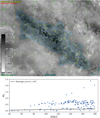 |
Fig. 10 Top: Gaia stars used for the extinction vs distance diagram of the Zebra1 nebula. The background is the total hydrogen column density in the velocity interval -9 km s-1 < vLSR < 4 km s-1 from Kalberla et al. (2020). Bottom: corresponding extinction vs. distance diagram. |
3.2 The Zebra1 nebula
The main pattern of the sky surface brightness distribution and of the N(H) and the AV maps is a network of sometimes curved cloud stripes. In the center of the field, however, we identified a large (6°.2 × 1°.2) area of higher extinction (Fig. 4). This region shows a maximum and average extinction of max(AV) = 1 and AV = 0.49, respectively. The average velocity of the background-foreground corrected H I 21 cm spectra at the N(H) peaks inside the Zebra1 area is  , with a total velocity dispersion of σ(vLSR) = 9 km s-1.
H I 21 cm spectra at one of these N(H) peaks are shown in Fig. 12.
The H I 21 cm line profile varies inside the Zebra1 region (see Appendix B), but it is a velocity-coherent structure, as seen in the H I channel maps from -8.2kms-1 to +0.8kms-1. We therefore conclude that it is an interstellar cloud, and we refer to it as the Zebra1 nebula. The main part of Zebra1 is best seen in the channel -3.3 km s-1, as shown in Fig. 13.
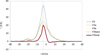 |
Fig. 12 H I 21 cm spectra in the direction of the N(H) peak F inside the Zebra1 nebula. ON (F0) and two OFF spectra (F0a and F0b are shown as well as the residual (F0total) calculated by subtracting the average of the OFF spectra (F0base) from the ON spectrum. A vertical line is drawn at vLSR = -3.3 km s-1). |
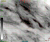 |
Fig. 13 H I 21 cm channel map (at vLSR = -3.3 km s-1) of the Zebra1 nebula and its surroundings from the GASS survey. The contours are at 18, 24, 30, and 36 K km s-1. An equatorial coordinate grid is overlaid. |
3.3 The distance of the Zebra1 nebula
When the extinction of a high galactic latitude cloud is similar to that shown by background stars, we can derive an upper limit for the distance of the cloud using the distances of these stars. The total number of Gaia DR3 stars in the 150□° region with AG ≥ 0.01mag and d < 180 pc is about 3600, so there should be about 175 inside the Zebra1 defining area, and we see 137. All the 109 Gaia stars with an extinction above the minimum visual extinction of AV,min = 0.31 in the Zebra1 nebula are at a distance of d > 75 pc. This is our first estimate for the upper limit of the distance. Accordingly, we searched for d < 75 pc break points in the Gaia-based extinction versus distance diagram of the Zebra1 nebula. By applying moving-average and curve fitting (see Fig. 14), we obtained 65 pc and 55 pc, respectively, for the probable distance for the Zebra1 nebula. The result is clearly affected by the very low number of nearby stars. We assumed that neighboring clouds with similar H I 21 cm velocities belong to the same ISM layer and so share the same distance. We united their extinction versus distance diagrams, as we did for the clouds seen at vLSR = -3.3 km s-1. The result confirmed the 60 pc distance.
 |
Fig. 14 Extinction vs distance diagram of the Zebra1 nebula zoomed into the 45 pc < d < 83 pc region with a moving-average (dotted line) and Gaussian fit (red continuous line) indicating a distance of about 60 pc. |
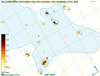 |
Fig. 15 CO(2–1) integrated line intensity at the head of the Zebra1 nebula from the Planck Legacy Archive. The contours at W = 0.7 K km s-1 peak at W = 0.7 K km s-1 An equatorial coordinate grid is overlaid. |
3.4 The size and mass of the Zebra1 nebula
The cPlat line-of-sight extent of the Zebra1 nebula was estimated from its apparent aPlat semimajor and bPlat semiminor axes, calculated from its angular size and dPlat distance as
 (3)
(3)
We accepted that cPlat < aPlat because the total velocity dispersion (σ(vLSR)) along the major axis of the cloud is larger than the FWHM line width.
The Tkin kinetic temperature of translucent clouds may vary in a broad range (100 K to few 1000 K). We followed Mattila (1979) to estimate Tkin from the H I 21 cm measurements.
An upper limit was derived from the ∆v line width as
![Mathematical equation: \sup T_\mathrm{kin}=(\frac{\Delta v}{0.214})^2 [\mathrm{K}].](/articles/aa/full_html/2025/09/aa54534-25/aa54534-25-eq8.png) (4)
(4)
With ∆v = 5K km s-1, this gives an upper limit of sup Tkin = 546 K, but we did not account for the turbulent broadening, so that the actual Tkin should be much lower. This means that the Zebra1 nebula is probably mostly neutral interstellar medium, and reliable mass estimates might be based on extinction and/or H I 21 cm observations.
The cloud is best seen in the H I channel maps from -8.2 kms-1 to +0.8 K km s-1, and the HI21 cm emission drops to the background level at vLSR = -9 km s-1 and 4 K km s-1. This was the velocity range for which we integrated the hydrogen column density corresponding to the Zebra1 nebula. We estimated the cloud mass using the total hydrogen column density estimates of Kalberla et al. (2020) and the Planck visual extinction data (see Table 2).
Interstellar clouds.
3.5 Other clouds
Our optical images indicated further bright nebulosities around the Zebra1 nebula. Multiwavelength sky surface brightness images show several associated bright regions in the region. We identified the Zebra1 neighborhood clouds as velocity-coherent structures using the H I channel maps, just as for the Zebra1 nebula. Some of them have the same LSR velocity as the Zebra1 nebula, such as the stripe seen NW of the Zebra1 (see Fig. 13). Some others are best seen at vLSR = -8.2 K km s-1 or at vLSR ≈ 0 K km s-1. Typically, these clouds have velocity gradients up to a few km s-1 mostly in the NE-SW direction. We calculated the main parameters of these clouds as for the Zebra1 nebula, and all are summarized in Table 2.
We collected data of the stars, which helped us to limit the distance of the Zebra1 nebula in Table 3. For a comparison, stars for the Zebra8 (Lower Cloud) and the LDN 1780 interstellar clouds are also shown there. Table 3 lists the nearest Gaia DR3 stars with some or considerable extinction, that is, with AG above the corresponding average AV value in the cloud (as derived from the Planck extinction maps). These background stars set an upper limit to the cloud distance. The columns of Table 3 are: (1) the name of the region; (2) related Gaia DR3 stars; (3) Gaia distance of the star; (4) Gaia G band extinction of the star; (5) V band extinction in the direction of the star as derived from Planck extinction maps; (6) our notes on the star selection. We selected the following stars for the regions in Table 3: (a) the nearest star with an AG value above the Parenago curve at the distance of the star; (b) the nearest star with an AG value above 3 times the value of the Parenago curve at the distance of the star; (c) the nearest star for which its Gaia AG based AV value exceeded the Planck based average AV value of the given region; (d) the star which showed the highest AG value up to a distance of 105pc; (e) the star which showed the highets AG value up to a distance of 180pc.
4 Discussion
4.1 Infrared appearance
Some extended surface brightness excess inside the W(H I) = 24 K km s-1 contour of the v( H I) = 3.3 Kkms-1 channel map of the Zebra1 nebula in the WISE (Wright et al. 2010) W3 (12 μm) and W4 (22 μm) images is visible, but it is not really visible at the shorter wavelengths (i.e., at 3.8 and 4.6 μm). In Fig. 16 we show the region of Zebra1 in the 12 μm WSSA (Meisner & Finkbeiner 2014) images, that is, in WISE band W3 data that are free of compact sources and contaminating artifacts. The 12 μm emission peaks apparently coincide with those of the extinction (see Fig. 4).
4.2 Other objects in the line of sight
Redfield & Linsky (2008) identified two clouds of the very local interstellar medium (VLISM) within 15 pc from the Sun in the direction of our field (in addition to the LIC): the GEM and NGP clouds. Their radial velocities are 36.3 km s-1 and 37.0 km s-1, respectively. These two structures are very extended, and their listed centers are well outside the studied region. Based on our Fig. 9, the contribution of any very local ISM to the Gaia extinctions is very small, AG(VLISM) < 0.02.
Searching for infrared excess clouds, Reach et al. (1998) combined data from the Cosmic Background Explorer Diffuse Infrared Background Experiment (COBE DIRBE) far-infrared and Leiden–Dwingeloo–Parkes H I 21 cm survey. They are located at an infrared excess of  at two positions in the region (see their Fig. 7a) at l = 334°, b = 39°.6, and at l = 332°, b = 38°. The first cloud coincides with the Zebra1 nebula, and the second cloud is 3 degrees SW of it, but the authors did not list these 0°.5 sized local peaks of far-IR excess in their catalog.
Stars limiting the distance of the interstellar clouds.
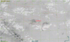 |
Fig. 16 12μm WSSA (Meisner & Finkbeiner 2014) image of the region of the Zebra1 nebula. The integrated intensity contours of the vLSR(H I) = -3.3 Kkm s-1) channel are overlaid, together with a galactic coordinate grid. |
4.3 The broad environment of the Zebra1 nebula
The ISM in the high-latitude region 25° ≤ b ≤ 47° at Galactic latitudes of 310° ≤ l ≤ 360° was not well studied so far (see the H I channel maps in Fig. 17).
The Redfield & Linsky (2008) survey listed DIR 316+39, a high Galactic latitude object with  similar to that at the Zebra1 nebula. DIR 316+39 has a diameter of 2° and a dust temperature of 18.8 K, which is typical for Galactic cirrus. LDN 1780 also appears there in their Fig. 7 with a size of 1.2 degrees and
  , but no infrared excess value is given in their Table 3, where it is listed as MBM 33.
DIR 316+39 was mapped by Onishi et al. (2001) using the NANTEN telescope, and a TR ≈ 1 K 12CO (J=1-0) line was detected. They did not report the line velocity, and we therefore accepted the vLSR = -1.6kms-1 velocity of the GASS survey H I 21 cm channel, in which the cloud is clearly visible.
We performed an extinction versus distance analysis for a circular area of 1.2 degrees around the center of the DIR 316+39 cloud. The first jump appears at 89 pc, where Gaia DR3 6195375361091393408 has AG = 0.6. This gives an upper limit for the distance of DIR 316+39.
LDN1778/1780 is the nearest member of a complex of high-latitude dark nebulae LDN134, LDN 169, LDN 183, and (see Lynds 1962; Mattila 1979; Clark & Johnson 1981; Hartmann et al. 1998). This group of high-latitude (|b| ≥ 25°) molecular clouds was also surveyed in CO(J = 2–1) by Magnani et al. (1985), who identified seven clouds. The complex is therefore also known as the MBM 33-MBM 39 (Fig. 15). Their velocities range from vLSR(MBM 38) = 0.8 km s-1 to vLSR(MBM 33) = 3.3kms-1. Toth et al. (1995) suggested that LDN 1780, which actually corresponds to MBM 33, might be part of the Loop I shells.
We performed an extinction versus distance analysis for the environment of the LDN 1780 cloud as well, which showed Gaia DR3 4397273833608878208 at 92pc with AG = 0.5 and five more stars with a similar extinction closer than 110 pc. Our distance estimate from the moving-average and curve fitting is dDIR3016+39 = 80 ± 10 pc, which agrees well with the  pc value derived by Zucker et al. (2019) using Gaia DR2.
We added the parameters of DIR 316+39 and LDN 1780 to Table 2 for comparison.
 |
Fig. 17 H I 21 cm channel maps of the high-latitude (25° ≤ b ≤ 47°) part of the Loop I from the GASS survey. The H I 21 cm line area is integrated in ∆v = 0.8 km s-1 channels centered at vLSR = -3.3 km s-1 vLSR = -0.8 km s-1 vLSR = 3.3 km s-1 in the left, center, and right image, respectively. The positions of the L1780, Zebra1 nebula and DIR316+39 are marked. A Galactic coordinate grid is overlaid. |
4.4 Clouds inside the Local Bubble
The cloud distances derived from curve fits are smaller by 10– 15pc than the distances of the nearest Gaia DR3 stars, with considerable extinction for the given cloud. All the clouds in Table 2. are inside the LB, even when we accept the upper limits as cloud distances. This means that there is a population of high-latitude clouds there that even has (see DIT306+39 and LDN1780; see, e.g., the Zebra1 nebula) molecular parts.
Estimating the 2c line-of-sight diameters of the clouds assuming  , we obtained a rough estimate of 60cm-2 < n(H) < 230cm-2 for the average volume densities of the Zebra clouds. This is larger by some orders of magnitude than the total hydrogen volume density of the local interstellar cloud and the other warm clouds of the VLISM that surround the Solar System with 0.1cm-2 < n(H) < 0.3cm-2 (see, e.g., Frisch et al. 1999; Redfield & Linsky 2008; Frisch et al. 2011; Linsky et al. 2022).
We compared the HI21 cm channel maps of a large (>50° × 25°) region to determine the relation of the Loop I to the Zebra1 nebula. Figure 17 shows the vLSR = 3.3 km s-1 (velocity of MBM 33, also know as LDN 1780); the vLSR = -0.8 km s-1 (velocity of DIR 316+39 of Reach et al. 1998) and vLSR = -3.3kms-1 (the velocity of the Zebra1 nebula). Based on their velocities, we cannot directly relate these objects to each other.
When we zoom out to a field of view that also includes the Galactic center region, these filamentary structures rather appear as a set of roughly concentric shells. The arcs visible above the Sco-Cen-Lup triple OB associations at higher Galactic latitudes might be cloud filaments that formed by shock waves in expanding bubble shells.
The little dips in some H I line profiles might be cause by self-absorption from cold (20 K) hydrogen gas, as shown by Burton et al. (1978). The H I gas kinetic temperature can then be calculated as well (see Koley & Roy 2019). The recent Parkes survey might also provide us with such data when it is published.
4.5 Uncertainties on deriving Tkin of the CNM
According to Heiles & Troland (2003), about 60% of all H I is in the warm neutral medium (WNM), and about half of the WNM has spin temperatures of 500–5000 K. We note that the upper limit we derived for the spin temperature of the Zebra1 nebula is close to this lower value. As a comparison, the column density weighted median for the CNM is 70 K.
We note, however, that the CNM is accumulated in sheets and not in spheres. When the turbulence is not isotropic, the calculation of the turbulent velocity distribution from the observed ΔvLOS line-of-sight velocity distribution is not straightforward. If the cloud were part of a sheet, we would need to know the sheet inclination angle (see Heiles & Troland 2003).
We also note that Liszt (2001) showed that hydrogen is not thermalized (TS < Tkin), and TS of the HI in CNM is hard to derive because we usually observe cold H I through a WNM with a range of temperatures.
5 Conclusions and outlook
We reported pattern of bright filamentary structures through optical imaging at high (b ≈ 40°) Galactic latitudes that we named Zebra nebula system because of its stripes.
We identified elongated interstellar clouds using multiwavelength data with moderate to average AG extinction.
The wall of the LB lies at a distance of about 135 pc in this direction, so that these clouds, which are all closer than 100 pc, must be located inside the LB.
Based on the H I 21 cm data, we cannot exclude that some of these nearby structures are related to the Loop I.
The most prominent cloud of the region, the Zebra1 nebula, lies at a distance of 60 ± 15 pc with a total mass of about 70(d/[60 pc])2 M⊙. This translucent cloud possible has a part in which hydrogen is molecular, that is, at its AV 1mag extinction peak position, where Planck CO(2–1) maps also indicate CO line emission.
Wide-field optical imaging of high Galactic latitude regions may help us to locate further nearby clouds even inside the LB. Future calibrated observations of the optical sky surface brightness in the region of the Zebra1 nebula and its neighborhood will allow us to correlate the cloud surface brightness with extinction, as was done by Mattila et al. (2018). A polarization study as was done for the MBM 33–39 complex by Neha et al. (2018), for example, would be helpful in understanding the 3D structure of the clouds in the Zebra1 region as well. Molecular line (CH, CO) observations of the AV 1 mag region of Zebra1 might also be carried out.
Acknowledgements
We are very grateful to the family Joachim and Adele Cranz for the possibility that we could conduct our campaign in their Isabis Astro Lodge on the Namibian Khomas Highland. We thank the valuable help of Ilona Mitró (Fornax Ltd., Pécel, Hungary) provided in Namibia, advises of Gábor Marton (Konkoly Thege Miklós Astronomical Institute, Budapest), and data management support by Victor Tóth. This research has made use of “Aladin sky atlas” developed at CDS, Strasbourg Observatory, France, Funding: This work was supported by the Office of Supported Research Groups of the Hungarian Research Network under the grant number HUN-REN-ELTE-0116607 Astropolarimetry.
Author Contributions: Substantial contributions to conception and design: JSB, AM, PS, LVT, GH; Performing experiments and data acquisition: JSB, AM, PS, GH; Data analysis and interpretation: JSB, AM, LVT, GH; Drafting the article or revising it critically for important intellectual content: JSB, AM, LVT, GH. Data Availability Statement: The data underlying this article are available in the article which has no supplementary material.
References
- Bonnarel, F., Fernique, P., Bienaymé, O., et al. 2000, A&AS, 143, 33 [NASA ADS] [CrossRef] [EDP Sciences] [Google Scholar]
- Bortle, J. E. 2001, S&T, 101, 126 [Google Scholar]
- Breitschwerdt, D., Feige, J., Schulreich, M. M., et al. 2016, Nature, 532, 73 [NASA ADS] [CrossRef] [Google Scholar]
- Burton, W. B., Liszt, H. S., & Baker, P. L. 1978, ApJ, 219, L67 [NASA ADS] [CrossRef] [Google Scholar]
- Clark, F. O., & Johnson, D. R. 1981, ApJ, 247, 104 [Google Scholar]
- Cox, D. P., & Reynolds, R. J. 1987, ARA&A, 25, 303 [NASA ADS] [CrossRef] [Google Scholar]
- Dharmawardena, T. E., Bailer-Jones, C. A. L., Fouesneau, M., et al. 2024, MNRAS, 532, 3480 [Google Scholar]
- Edenhofer, G., Zucker, C., Frank, P., et al. 2024, A&A, 685, A82 [NASA ADS] [CrossRef] [EDP Sciences] [Google Scholar]
- Frisch, P. C., Dorschner, J. M., Geiss, J., et al. 1999, ApJ, 525, 492 [NASA ADS] [CrossRef] [Google Scholar]
- Frisch, P. C., Redfield, S., & Slavin, J. D. 2011, ARA&A, 49, 237 [CrossRef] [Google Scholar]
- Gaia Collaboration (Brown, A. G. A., et al.) 2018, A&A, 616, A1 [NASA ADS] [CrossRef] [EDP Sciences] [Google Scholar]
- Gaia Collaboration (Brown, A. G. A., et al.) 2021, A&A, 649, A1 [NASA ADS] [CrossRef] [EDP Sciences] [Google Scholar]
- Güver, T., & Özel, F. 2009, MNRAS, 400, 2050 [Google Scholar]
- Hartmann, D., Magnani, L., & Thaddeus, P. 1998, ApJ, 492, 205 [Google Scholar]
- Heiles, C., & Troland, T. H. 2003, ApJ, 586, 1067 [NASA ADS] [CrossRef] [Google Scholar]
- HI4PI Collaboration (Ben Bekhti, N., et al.) 2016, A&A, 594, A116 [NASA ADS] [CrossRef] [EDP Sciences] [Google Scholar]
- Jordi, C., Gebran, M., Carrasco, J. M., et al. 2010, A&A, 523, A48 [NASA ADS] [CrossRef] [EDP Sciences] [Google Scholar]
- Kalberla, P. M. W., & Haud, U. 2015, A&A, 578, A78 [NASA ADS] [CrossRef] [EDP Sciences] [Google Scholar]
- Kalberla, P. M. W., Kerp, J., & Haud, U. 2020, A&A, 639, A26 [EDP Sciences] [Google Scholar]
- Koley, A., & Roy, N. 2019, MNRAS, 483, 593 [CrossRef] [Google Scholar]
- Lallement, R., Babusiaux, C., Vergely, J. L., et al. 2019, A&A, 625, A135 [NASA ADS] [CrossRef] [EDP Sciences] [Google Scholar]
- Leike, R. H., Glatzle, M., & Enßlin, T. A. 2020, A&A, 639, A138 [NASA ADS] [CrossRef] [EDP Sciences] [Google Scholar]
- Linsky, J. L., & Redfield, S. 2021, ApJ, 920, 75 [Google Scholar]
- Linsky, J., Redfield, S., Ryder, D., & Moebius, E. 2022, Space Sci. Rev., 218, 16 [Google Scholar]
- Liszt, H. 2001, A&A, 371, 698 [NASA ADS] [CrossRef] [EDP Sciences] [Google Scholar]
- Lynds, B. T. 1962, ApJS, 7, 1 [NASA ADS] [CrossRef] [Google Scholar]
- Magnani, L., Blitz, L., & Mundy, L. 1985, ApJ, 295, 402 [NASA ADS] [CrossRef] [Google Scholar]
- Maheswar, G., Lee, C. W., Bhatt, H. C., Mallik, S. V., & Dib, S. 2010, A&A, 509, A44 [NASA ADS] [CrossRef] [EDP Sciences] [Google Scholar]
- Mattila, K. 1970, A&A, 9, 53 [NASA ADS] [Google Scholar]
- Mattila, K. 1979, A&A, 78, 253 [NASA ADS] [Google Scholar]
- Mattila, K., Haas, M., Haikala, L. K., et al. 2018, A&A, 617, A42 [NASA ADS] [CrossRef] [EDP Sciences] [Google Scholar]
- McClure-Griffiths, N. M., Pisano, D. J., Calabretta, M. R., et al. 2009, ApJS, 181, 398 [NASA ADS] [CrossRef] [Google Scholar]
- Meisner, A. M., & Finkbeiner, D. P. 2014, ApJ, 781, 5 [Google Scholar]
- Neha, S., Maheswar, G., Soam, A., & Lee, C. W. 2018, MNRAS, 476, 4442 [NASA ADS] [CrossRef] [Google Scholar]
- O’Neill, T. J., Zucker, C., Goodman, A. A., & Edenhofer, G. 2024, ApJ, 973, 136 [NASA ADS] [CrossRef] [Google Scholar]
- Onishi, T., Yoshikawa, N., Yamamoto, H., et al. 2001, PASJ, 53, 1017 [NASA ADS] [Google Scholar]
- Parenago, P. P. 1945, Popul. Astron., 53, 441 [Google Scholar]
- Planck Collaboration Int. XXIX. 2016, A&A, 586, A132 [NASA ADS] [CrossRef] [EDP Sciences] [Google Scholar]
- Reach, W. T., Wall, W. F., & Odegard, N. 1998, ApJ, 507, 507 [CrossRef] [Google Scholar]
- Redfield, S., & Linsky, J. L. 2008, ApJ, 673, 283 [Google Scholar]
- Redfield, S., & Linsky, J. L. 2015, ApJ, 812, 125 [Google Scholar]
- Rybarczyk, D. R., Wenger, T. V., & Stanimirovic´, S. 2024, ApJ, 975, 167 [Google Scholar]
- Sanders, W. T., Kraushaar, W. L., Nousek, J. A., & Fried, P. M. 1977, ApJ, 217, L87 [Google Scholar]
- Sharov, A. S. 1964, Soviet Ast., 7, 689 [Google Scholar]
- Slíz-Balogh, J., Mádai, A., Sári, P., Barta, A., & Horváth, G. 2024, MNRAS, 530, 3570 [Google Scholar]
- Straižys, V., Boyle, R. P., Zdanavicˇius, J., et al. 2018, A&A, 611, A9 [NASA ADS] [CrossRef] [EDP Sciences] [Google Scholar]
- Toth, L. V., Haikala, L. K., Liljestroem, T., & Mattila, K. 1995, A&A, 295, 755 [NASA ADS] [Google Scholar]
- Welsh, B. Y., & Shelton, R. L. 2009, Ap&SS, 323, 1 [NASA ADS] [CrossRef] [Google Scholar]
- Wright, E. L., Eisenhardt, P. R. M., Mainzer, A. K., et al. 2010, AJ, 140, 1868 [Google Scholar]
- Yan, Q.-Z., Yang, J., Sun, Y., Su, Y., & Xu, Y. 2019, ApJ, 885, 19 [NASA ADS] [CrossRef] [Google Scholar]
- Zdanavicˇius, J., Vrba, F. J., Zdanavicˇius, K., Straižys, V., & Boyle, R. P. 2011, Baltic Astron., 20, 1 [Google Scholar]
- Zucker, C., Speagle, J. S., Schlafly, E. F., et al. 2019, ApJ, 879, 125 [NASA ADS] [CrossRef] [Google Scholar]
- Zucker, C., Goodman, A. A., Alves, J., et al. 2022, Nature, 601, 334 [NASA ADS] [CrossRef] [Google Scholar]
Appendix A The Parenago formula
Parenago (1945) proposed a relatively simple formula for describing the interstellar extinction as a function of distance (r) and galactic latitude (b). The Parenago curve models the distance dependence of extinction assuming a constant scale height of β for the exponential distribution of the diffuse component of interstellar dust in the Galactic plane, and a factor a0 for the extinction per kiloparsec in the Galactic plane:
 (A.1)
(A.1)
where Parenago (1945) assumed a0 = 3.5mag/kpc, β= 100 ± 4 pc, ε = 0.25mag A careful investigation of the formula (A.1) was carried out by Sharov (1964). A significant galactic latitude dependence of a0 were found at low galactic latitudes |b| < 10° with a whole sky mean of a0 = 1.6mag/kpc. Besides a slight variation of the scale height 100 pc ≳ β ≳ 140 pc was found with the minimum at l ≈ 180° and maximum at l ≈ 0°. We applied a0 = 1.25mag/kpc i.e. the value used also by Zdanavičius et al. (2011) and Straižys et al. (2018), and β = 130 pc.
Appendix B Extinction-distance studies of the clouds
We prepared extinction versus distance diagrams for the filamentary clouds (velocity coherent structures of enhanced extinction) in the studied region. We present pairs of figures: the first one indicates the position of Gaia stars included in the scatter plot of the second one.
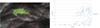 |
Fig. B.1 Extinction vs distance diagram for the Zebra7 (Top Cloud) (right) and the Gaia stars used (left). We note that the Zebra7 is a large cloud, and most of it lays outside the studied area. |
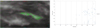 |
Fig. B.2 Extinction vs distance diagram for the Zebra5 (Front Cloud) (right) and the Gaia stars used (left). |
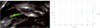 |
Fig. B.3 Extinction vs distance diagram for Zebra6 (Rear Cloud) (right) and the Gaia stars used (left). |
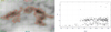 |
Fig. B.4 Extinction vs distance diagram for the Zebra8 (Lower Cloud) (right) and the Gaia stars used (left.) |
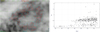 |
Fig. B.5 Extinction vs distance diagram for the Zebra9 (Lower Ring) cloud (right) and the Gaia stars used (left). |
Appendix C H I 21 cm spectra of the clouds
Local maxima of hydrogen column density were defined in Fig. 6 and the 2/3N(H)max contours were drawn for each peaks. Then background- and foreground-subtracted average H I 21 cm spectra were derived for all these peak regions from A to Z. All these spectra are presented here.
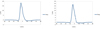 |
Fig. C.1 Background- and foreground-subtracted H I 21 cm spectra of peaks A and B. |
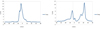 |
Fig. C.2 Background- and foreground-subtracted H I 21 cm spectra of peaks C and D. |
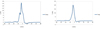 |
Fig. C.3 Background- and foreground-subtracted H I 21 cm spectra of peaks E and F. |
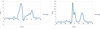 |
Fig. C.4 Background- and foreground-subtracted H I 21 cm spectra of peaks G and H. |
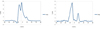 |
Fig. C.5 Background- and foreground-subtracted H I 21 cm spectra of peaks I and J. |
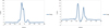 |
Fig. C.6 Background- and foreground-subtracted H I 21 cm spectra of peaks K and L. |
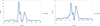 |
Fig. C.7 Background- and foreground-subtracted H I 21 cm spectra of peaks M and N. |
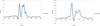 |
Fig. C.8 Background- and foreground-subtracted H I 21 cm spectra of peaks O and P. |
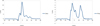 |
Fig. C.9 Background- and foreground-subtracted H I 21 cm spectra of peaks Q and R. |
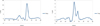 |
Fig. C.10 Background- and foreground-subtracted H I 21 cm spectra of peaks S and T. |
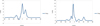 |
Fig. C.11 Background- and foreground-subtracted H I 21 cm spectra of peaks U and V. |
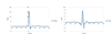 |
Fig. C.12 Background- and foreground-subtracted H I 21 cm spectra of peaks W and X. |
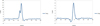 |
Fig. C.13 Background- and foreground-subtracted H I 21 cm spectra of peaks Y and Z. |
AIfA H I Surveys Data Server https://www.astro.uni-bonn.de/hisurvey/index.php
All Tables
All Figures
|
Fig. 1 Measurement site of our observations at the Isabis Astro Lodge in the Namibian Khomas Highland with our portable telescope. Photo by Pál Sári. |
| In the text | |
|
Fig. 2 Relative quantum efficiency of the CMOS camera sensor of our polarimetric telescope as a function of wavelength (nm). |
| In the text | |
|
Fig. 3 Photometric images of the region in the constellation Libra. The size of the images is 15°.26 × 10°.18. The brightest star in the images is the spectroscopic binary alf02 Lib at RA = 14h50m52.71s Dec = -16°02′30″.4. Top: picture center at RA = 14h36m47s, Dec = -16°28′26″) taken on 21 July 2023 at 18:24:57 UT. Middle: picture center at RA = 14h56m47s, Dec = -16°28′26″ taken on 21 July 2023 at 18:44:58. Bottom: picture center at RA = 14h41m47s, Dec = -16°28′26″ taken on 23 July 2023 at 18:58:54 UT. Photos by Judit Slíz-Balogh and Attila Mádai. |
| In the text | |
|
Fig. 4 AV_RQ (V band) visual extinction map from the Planck Legacy Archive centered on RA = 14h40m, Dec = -16°. The contours are drawn at 0.3, 0.38, 0.46, 0.54, 0.62, and 0.7 magnitudes. The Zebra nebula is shown roughly in the middle. An equatorial coordinate grid is overlaid. |
| In the text | |
|
Fig. 5 Sample GASS (Kalberla & Haud 2015) H I 21 cm spectrum from the HI4PI archive at l = 336° 137, b = 40°.257 RA = 14h34m27.4s, Dec = -15° 52′48″. |
| In the text | |
|
Fig. 6 Total hydrogen column density distribution based on the full sky H I survey by HI4PI Collaboration (2016). The boundary of the optical frame is overlaid (yellow). Gaia stars with a G-band extinction of AG ≥ 0.3 Gaia at a distance of d ≤ 80 pc are overplotted (filled red circles). |
| In the text | |
|
Fig. 7 Distance vs extinction diagram based on 3822 stars in the Gaia DR3 taken from the sky window (14h06m 17s ≤ RA ≤ 15h07m 17s, -21°33′50″≤ DE ≤ -11°23′2″), as Fig. 3(A). The vertical red lines mark break points at about 60, 80, and 120 pc. |
| In the text | |
|
Fig. 8 Distance vs. extinction diagram based on the Gaia DR3 taken from the sky window of Fig. 3(A), but limited to distances d < 100 pc. The vertical red lines mark the break points at about 60 and 80 pc. |
| In the text | |
|
Fig. 9 Distance vs. extinction diagram based on the Gaia DR3 taken from the sky window of Fig. 3(A), but limited to distances d < 100 pc and extinctions AG < 0.1. |
| In the text | |
|
Fig. 10 Top: Gaia stars used for the extinction vs distance diagram of the Zebra1 nebula. The background is the total hydrogen column density in the velocity interval -9 km s-1 < vLSR < 4 km s-1 from Kalberla et al. (2020). Bottom: corresponding extinction vs. distance diagram. |
| In the text | |
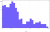 |
Fig. 11 Distribution of the Gaia DR3 AG extinction values of the stars in Fig. 7 |
| In the text | |
|
Fig. 12 H I 21 cm spectra in the direction of the N(H) peak F inside the Zebra1 nebula. ON (F0) and two OFF spectra (F0a and F0b are shown as well as the residual (F0total) calculated by subtracting the average of the OFF spectra (F0base) from the ON spectrum. A vertical line is drawn at vLSR = -3.3 km s-1). |
| In the text | |
|
Fig. 13 H I 21 cm channel map (at vLSR = -3.3 km s-1) of the Zebra1 nebula and its surroundings from the GASS survey. The contours are at 18, 24, 30, and 36 K km s-1. An equatorial coordinate grid is overlaid. |
| In the text | |
|
Fig. 14 Extinction vs distance diagram of the Zebra1 nebula zoomed into the 45 pc < d < 83 pc region with a moving-average (dotted line) and Gaussian fit (red continuous line) indicating a distance of about 60 pc. |
| In the text | |
|
Fig. 15 CO(2–1) integrated line intensity at the head of the Zebra1 nebula from the Planck Legacy Archive. The contours at W = 0.7 K km s-1 peak at W = 0.7 K km s-1 An equatorial coordinate grid is overlaid. |
| In the text | |
|
Fig. 16 12μm WSSA (Meisner & Finkbeiner 2014) image of the region of the Zebra1 nebula. The integrated intensity contours of the vLSR(H I) = -3.3 Kkm s-1) channel are overlaid, together with a galactic coordinate grid. |
| In the text | |
|
Fig. 17 H I 21 cm channel maps of the high-latitude (25° ≤ b ≤ 47°) part of the Loop I from the GASS survey. The H I 21 cm line area is integrated in ∆v = 0.8 km s-1 channels centered at vLSR = -3.3 km s-1 vLSR = -0.8 km s-1 vLSR = 3.3 km s-1 in the left, center, and right image, respectively. The positions of the L1780, Zebra1 nebula and DIR316+39 are marked. A Galactic coordinate grid is overlaid. |
| In the text | |
|
Fig. B.1 Extinction vs distance diagram for the Zebra7 (Top Cloud) (right) and the Gaia stars used (left). We note that the Zebra7 is a large cloud, and most of it lays outside the studied area. |
| In the text | |
|
Fig. B.2 Extinction vs distance diagram for the Zebra5 (Front Cloud) (right) and the Gaia stars used (left). |
| In the text | |
|
Fig. B.3 Extinction vs distance diagram for Zebra6 (Rear Cloud) (right) and the Gaia stars used (left). |
| In the text | |
|
Fig. B.4 Extinction vs distance diagram for the Zebra8 (Lower Cloud) (right) and the Gaia stars used (left.) |
| In the text | |
|
Fig. B.5 Extinction vs distance diagram for the Zebra9 (Lower Ring) cloud (right) and the Gaia stars used (left). |
| In the text | |
|
Fig. C.1 Background- and foreground-subtracted H I 21 cm spectra of peaks A and B. |
| In the text | |
|
Fig. C.2 Background- and foreground-subtracted H I 21 cm spectra of peaks C and D. |
| In the text | |
|
Fig. C.3 Background- and foreground-subtracted H I 21 cm spectra of peaks E and F. |
| In the text | |
|
Fig. C.4 Background- and foreground-subtracted H I 21 cm spectra of peaks G and H. |
| In the text | |
|
Fig. C.5 Background- and foreground-subtracted H I 21 cm spectra of peaks I and J. |
| In the text | |
|
Fig. C.6 Background- and foreground-subtracted H I 21 cm spectra of peaks K and L. |
| In the text | |
|
Fig. C.7 Background- and foreground-subtracted H I 21 cm spectra of peaks M and N. |
| In the text | |
|
Fig. C.8 Background- and foreground-subtracted H I 21 cm spectra of peaks O and P. |
| In the text | |
|
Fig. C.9 Background- and foreground-subtracted H I 21 cm spectra of peaks Q and R. |
| In the text | |
|
Fig. C.10 Background- and foreground-subtracted H I 21 cm spectra of peaks S and T. |
| In the text | |
|
Fig. C.11 Background- and foreground-subtracted H I 21 cm spectra of peaks U and V. |
| In the text | |
|
Fig. C.12 Background- and foreground-subtracted H I 21 cm spectra of peaks W and X. |
| In the text | |
|
Fig. C.13 Background- and foreground-subtracted H I 21 cm spectra of peaks Y and Z. |
| In the text | |
Current usage metrics show cumulative count of Article Views (full-text article views including HTML views, PDF and ePub downloads, according to the available data) and Abstracts Views on Vision4Press platform.
Data correspond to usage on the plateform after 2015. The current usage metrics is available 48-96 hours after online publication and is updated daily on week days.
Initial download of the metrics may take a while.