| Issue |
A&A
Volume 701, September 2025
|
|
|---|---|---|
| Article Number | A229 | |
| Number of page(s) | 8 | |
| Section | Stellar structure and evolution | |
| DOI | https://doi.org/10.1051/0004-6361/202554666 | |
| Published online | 16 September 2025 | |
Magnetar outburst models with cooling simulations
1
Institute of Space Sciences (ICE-CSIC), Campus UAB, C/ de Can Magrans s/n, Cerdanyola del Vallès (Barcelona), 08193
Spain
2
Institut d’Estudis Espacials de Catalunya (IEEC), 08034 Barcelona, Spain
3
Gran Sasso Science Institute (GSSI), Viale F. Crispi 7, L’Aquila, 67100
Italy
4
Departament de Física Aplicada, Universitat d’Alacant, Ap. Correus 99, E-03080 Alacant, Spain
5
Department of Physics and Astronomy, University of Padova, Via Marzolo 8, I-35131 Padova, Italy
6
Mullard Space Science Laboratory, University College London, Holmbury St. Mary, Surrey, RH5 6NT
United Kingdom
⋆ Corresponding author: This email address is being protected from spambots. You need JavaScript enabled to view it.
Received:
20
March
2025
Accepted:
25
July
2025
Abstract
Magnetar outbursts are among the most noteworthy manifestations of magnetism in neutron stars. They are episodes in which the X-ray luminosity of a strongly magnetised neutron star swiftly rises by several orders of magnitude to then decay over the course of several months. In this work, we present simulations of outbursts as a consequence of localised heat deposition in a magnetised neutron star crust, and the subsequent surface cooling. In particular, we employed a magnetothermal evolution code adapted to the study of short-term phenomena; that is, one including in its integration domain the outer layers of the star, where heat diffusion is faster. This choice entailed the development and use of heat blanketing envelope models that are thinner than those found in the literature as the surface boundary condition. We find that such envelopes can support a higher surface temperature than the thicker ones (albeit for less time), which can account for the typical luminosities observed in outbursts even when coming from small hotspots (few km in radius). We study several parameters related to the energetics and geometry of the heating region, concluding that the cooling of a crustal hotspot found in the outer part of the crust can account for the luminosity evolution observed in outbursts both in terms of peak luminosity and timescales. Finally, we discuss the key observables that must be studied in future observations to better constrain the nature of the underlying mechanism.
Key words: neutrinos / stars: magnetars / stars: neutron
© The Authors 2025
 Open Access article, published by EDP Sciences, under the terms of the Creative Commons Attribution License (https://creativecommons.org/licenses/by/4.0), which permits unrestricted use, distribution, and reproduction in any medium, provided the original work is properly cited.
This article is published in open access under the Subscribe to Open model. This email address is being protected from spambots. You need JavaScript enabled to view it. to support open access publication.
1. Introduction
One of the most conspicuous traits of neutron stars (NSs) is their extremely strong magnetic fields, which are inferred to range from several millions up to ≈1015 G. At the higher end of this range are found the so-called magnetars, objects powered by their ultra-strong magnetic field; they manifest themselves as soft gamma repeaters (SGRs) and anomalous X-ray pulsars (AXPs), though this distinction is by now largely obsolete (Duncan & Thompson 1992, see the reviews by Mereghetti et al. 2015; Turolla et al. 2015; Kaspi & Beloborodov 2017; Esposito et al. 2021). Many magnetars have been observed to undergo outbursts, that is, phases of enhanced X-ray luminosity that last from several months to years (Rea & Esposito 2011; Coti Zelati et al. 2018). Indeed, the discovery of new sources often occurs during an outburst. In some cases, the same source went through several outbursts separated by years of quiescence, such as, most recently, SGR 1935+2154 (Israel et al. 2016; Ibrahim et al. 2024), XTE J1810−197 (Borghese et al. 2021), CXOU J164710.2−455216 (Borghese et al. 2019) and 1E 1547−5408 (Bernardini et al. 2011; Coti Zelati et al. 2020). Overall, ∼30 outbursts have been observed to date1.
Typically, the enhancement of the luminosity is accompanied by an increased flaring activity, with the emission of several short bursts in the first few hours of the outburst as well as by timing anomalies such as glitches (e.g. Kaspi & Beloborodov 2017). Recently, the latest outburst of SGR 1935+2154 attracted renewed attention to these phenomena, as two short radio bursts were detected in temporal and spatial coincidence with it (CHIME/FRB Collaboration 2020; Bochenek et al. 2020; Mereghetti et al. 2020), reinforcing the idea of an association between magnetar outbursts and at least some fast radio bursts (e.g. Caleb & Keane 2021; Petroff et al. 2022, but several alternative scenarios have been proposed, e.g. Sridhar et al. 2021). From a spectral standpoint, the X-ray emission of magnetars can generally be described as the combination of a thermal component (one or more blackbodies associated with the emission from the surface) plus a power law with a photon index ∼2–4 (associated with processes in the magnetosphere). The flux enhancement during an outburst corresponds to a hardening of this spectrum that is typically well fit by a further blackbody (e.g. Rea & Esposito 2011). The equivalent emission radius of this component is much smaller than that of the whole stellar surface (typically ≲3 km). Concurrently, the pulsed fraction rises substantially. This provides evidence that outbursts are associated with the appearance of overheated regions in the NS crust. Moreover, the timescale for heat diffusion in the outer crust (where densities are lower than the neutron drip one ρND ≈ 4 × 10¹¹ g cm−3) matches that of the duration of outbursts.
These factors concur with the idea that outbursts are caused by some kind of abrupt event liberating a large amount of heat in or just above the NS crust, likely magnetic in origin. The exact nature of this trigger is still debated, in particular whether it originates from within the crust or it is the result of the activity in the magnetosphere (e.g. Beloborodov 2009; Carrasco et al. 2019). In particular, in the former case the energy release is thought to follow a star-‘quake’ caused by the accumulation of magnetic stress due for example to the Hall effect (e.g. Dehman et al. 2020, and references therein) or a MHD instability related to it (Gourgouliatos & Pons 2019), possibly mediated by a thermoplastic wave (Li et al. 2016; Lander 2023). In this scenario, outbursts amount to a substantial crustal heating and the subsequent cooling, and they can hence be studied within the formalism of magneto-thermal evolution of NS crusts. This approach has been first employed by Pons & Rea (2012, in the following PR+12), using an early model in axial symmetry. Subsequent works have improved on this approach by enhancing the detail of the microphysics treatment (Deibel et al. 2017, which is based on a 1D MESA model) or expanding the scheme to three dimensions, albeit in a set-up with a simplified description of the microphysics (De Grandis et al. 2022). In this work, we revisit and expand the 2D approach with a more robust code, including a state-of-the-art microphysics input and extending the integration domain to low densities in order to consistently treat short-term events; moreover, we pave the way for detailed 3D modelling with recently developed numerical tools (Dehman et al. 2023; Ascenzi et al. 2024). In particular, in Sect. 2 we outline the adaptations we made to the cooling code for the study of short-term phenomena, with a particular focus on the choice of the envelope models (i.e. the boundary condition for the thermal evolution equation); we then proceed in Sect. 3 to relate different observables to the parameters of our model, in particular those regarding the energetics (Sect. 3.1, 3.2) and the geometry (Sect. 3.3) of the heat source; we then discuss our findings and draw our conclusions in Sect. 4.
2. Methods
2.1. Physics input and numerical set-up
We employed a suitably adapted version of the 2D magnetothermal evolution code described in Viganò et al. (2021), which solves the coupled thermal and magnetic evolution of a NS in an axisymmetric set-up. The hydrostatic structure of the star was calculated self-consistently solving the TOV equation (e.g. Thorne 1977) supplemented by the BSk24 equation of state (Pearson et al. 2019) as found in the CompOSE catalogue (Typel et al. 2015)2.
In particular, the evolution of the temperature was found by solving the thermal evolution equation in the form
![Mathematical equation: $$ \begin{aligned} c_\text{v}\frac{\partial (\text{ e}^\nu T)}{\partial t}=\nabla \cdot \left[\text{ e}^{\nu }\,\hat{\kappa }\cdot \nabla (\text{ e}^\nu T)\right] + \text{ e}^{2\nu }(H-Q_\nu ), \end{aligned} $$](/articles/aa/full_html/2025/09/aa54666-25/aa54666-25-eq1.gif) (1)
(1)
where cv is the specific heat, eν is the general-relativistic metric factor calculated assuming a Schwarzschild metric (the operator ∇ also contains a relativistic correction),  the thermal conductivity tensor, H is a heating term, and Qν the neutrino emissivity. The term H is akin to the one included in long-term cooling simulations to describe effects such as the heating coming from ohmic dissipation. In this instance, we activated it in a localised region of the crust (see Sect. 3) and a short time period as a means to describe the heating associated with the activation of an outburst, without exactly specifying the nature of the trigger.
We adopted calculations of the transport coefficients described in Potekhin et al. (2015) in their latest implementation available online3. The neutrino emissivities are described according to Yakovlev et al. (2001); in particular, whereas the long-term cooling of a NS is controlled by the neutrino reactions happening in its core (Page et al. 2004), when studying the thermal evolution of hotspots located in the crust it becomes fundamental to consider those happening in the crust itself. These are non-negligible only if the temperature is above ≳109 K, and hence are only important in the very early phases of ordinary cooling. However, their dependence on temperature is very steep, so that they are able to limit the maximum possible temperature that in a NS crust close to their activation threshold.
Within the present axially symmetric set-up, we are only able to consider outbursts originating at one of the magnetic poles so that the heated region has a spot-like rather than a ring-like structure (which would alter the geometric relation between heated volume and emitting surface). The heating term, H, in Eq. (1) is therefore defined in terms of five parameters: the total energy input, Einj, the injection time, tinj, and three values defining the geometry of the heated region. Namely, we consider a truncated cone centred around the pole, defined by its radius R (referred to the z axis) and the inner and outer depths, counted from the crust-envelope interface (i.e. the external boundary of the grid), zin (towards the centre) and zout (towards the surface). In order to avoid numerically problematic sharp time gradients, the energy injection was modulated by a sinusoidal function in time; we tested other modulation profiles (such as a Gaussian), finding only very marginal differences in the shape of the luminosity curves near their peaks.
In the present study, we did not consider the evolution of the magnetic field, but rather fix it in a configuration that for simplicity we chose to be dipolar, akin to the one described in Aguilera et al. (2008). Assuming no magnetic evolution over our simulations is reasonable since the magnetic field evolves over a timescales that are much longer that the months to years studied here. This assumption also amounts to disregarding any change in the field that is associated with the onset of the outburst itself, which reflects the choice of not considering a concrete trigger model (itself due to the lack of a viable picture in the literature). In the present set-up, hence, the magnetic field acts as a bystander to the cooling of the hotspot. A more complete assessment of its role is beyond our present scope, as it would require both a sound microphysical treatment of the heating phase and a 3D framework (see Sect. 4 for a more detailed assessment of the impact of the magnetic field on our results). Note that we keep the full dependencies of the microphysical quantities on the (fixed) magnetic field, most notably through the thermal conductivity and weak-synchrotron neutrino emission, even though it did not get evolved itself.
2.2. Blanketing envelope models
In the outermost stellar layers, density drops by several orders of magnitude within several tens of meters. The temperature also shows a steep gradient, dropping by about two orders of magnitude across this optically thick but geometrically thin layer. Hence, it is problematic to include this region in a computational domain together with the rest of the NS. Rather, it is standard practice to solve its thermal structure separately, to then use the result of this operation to set a Neumann-type outer boundary condition for the heat equation. Within this approach, the outermost layers are referred to as a heat blanketing envelope. In particular, an envelope model gets implemented as a relation between the temperature Tb at the bottom of the envelope (i.e. at the top of the crust) and Ts at the surface.
Several relations of this kind have been computed in the literature, the most well known being the one obtained by Gudmundsson et al. (1983) for an unmagnetised heavy-element envelope in plane-parallel approximation. Several alternatives, including ones accounting, for instance, for different chemical composition or magnetic fields, are found in the literature (see the review by Beznogov et al. 2021). However, the vast majority of the Tb–Ts relations available for application in cooling codes are adapted to the long-term evolution of NSs only. In fact, the assumption underlying the separation of the envelope from the rest of the integration domain is that the heat diffusion across the envelope itself should happen faster than the individual timestep of the simulation. Therefore, the thickness of the envelope sets the time resolution of the cooling simulation, and in order to study short-term phenomena it becomes necessary to consider a thinner envelope. At the same time, this operation moves a larger portion of the NS crust within the integration domain of the (in this case, 2D) magnetothermal code, so that the evolution of lower-density layers, where heat diffusion is faster, can be described with the full Eq. (1) rather than in the plane-parallel, stationary approximation. We then proceed to build our own Tb–Ts relations for envelopes that are thinner than those available in the literature taking into account the effects of a strong magnetic field.
We followed closely the formalism in Potekhin et al. (2007, see also Thorne 1977), producing a set of models of the outer stellar layers for different values of surface temperatures Ts, magnetic field strength and orientation of the field itself with respect to the radial direction. The integration of the corresponding system of differential equations proceeds up to a density ρb that sets the thickness of the envelope. Whereas most models in the literature set ρb = 1010 g cm−3, we considered densities reaching down to ρb ≈ 107 g cm−3, so that the time resolution of the simulation goes down from the timescale of the year to that of the hour. These thinner envelopes are able to support larger values of the surface temperature for the same Tb, which cannot be sustained for a longer time in a stationary fashion. Some examples of how different choices of ρb reflect on the Tb–Ts relation are shown in Fig. 1. Moreover, the maximum surface temperature is also controlled by neutrino emission in the envelope itself. This effect was described by Potekhin et al. (2015) as an asymptotic limit to the Tb–Ts relation (shaded magenta area in Fig. 1). However, neutrino emissivity is significant only at densities above ≈108 g cm−3, so that for thinner envelopes this effect is not as important.
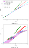 |
Fig. 1. Tb–Ts relations calculated for a sample of representative values of Ts in the case of Fe envelopes. Different colours and markers denote different bottom-of-the-envelope densities ρb. The models from Gudmundsson et al. (1983) and Potekhin et al. (2015), calculated for the standard value ρb = 1010 g cm−3, are plotted for reference. The spread of the points at the same Ts (which is noticeable only in the bottom panel) corresponds to different ΘB, with higher Tb giving a lower Ts value for the same Tb. Two values for the magnetic field, 108 G (top panel) and 1012 G (bottom panel) are shown; these values have been chosen, although comparatively low, for clarity of visualisation, as stronger fields yield very sparse plots. |
We built models of a thin (ρb ≈ 107 g cm−3), magnetised blanketing envelopes for two extreme cases of their chemical composition (Fe or H) and implemented them within our cooling code with a formalism that allows flexibility in ρb, as well as in Tb and B. Namely, we encapsulated our Tb–Ts relation in a single-layer neural network, trained on a set of envelope models that replaces an analytical fit. We refer to a companion paper (Kovlakas et al. 2025) for details about this implementation, and about the construction of the envelope models themselves.
3. Results
In this section, we present a range of models of heat injection and subsequent cooling, varying the parameters associated with the heating itself, Einj and tinj, and the geometry of the interested region zin, zout and R. We will also address the role of the background state, in particular considering different NS masses.
3.1. Increasing the energy input: Luminosity saturation
PR+12 observed that the peak luminosity of an outburst is capped by the steeply increasing efficiency of neutrino emissivity from the crust when the temperature gets above ≈3 × 10⁹ K. This is in line with the observational fact that the luminosity of outbursts does not exceed a value of about 1036 erg/s. However, the exact value crucially depends on the size of the heated region, as well as on the employed envelope model.
To reassess this result in our more consistent set-up, we considered models with increasing Einj, for which we show in Fig. 2 the evolution of photon and neutrino luminosity. Here, we kept a fixed injection time tinj = 10 h and geometry, zin = 400 m, zout = 5 m, R = 3 km ; an analysis of the role of these other parameters follows in the next subsections. Indeed, we can observe that as Einj increases the photon luminosity curves get piled up at a limit value of about 1036 erg/s. We tested two different envelope compositions, one of pure Fe and the other of pure H (representing the two extreme scenarios, see Kovlakas et al. 2025), finding just a small difference in the two cases. This is due to the fact that at very high temperature the thermal structure of the envelope itself is regulated by neutrino emission, so that the composition becomes less important.
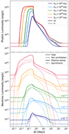 |
Fig. 2. (Top panel) Photon luminosity with growing heat injection, in the case of Fe (solid lines) or H (dashed lines) envelopes. (Bottom panel) Corresponding neutrino luminosity, with its dominant channels: a continuous line indicates the total Lν, dashed lines the contribution from e+e− pair annihilation, dotted lines the one from plasmon decay, and the dash-dotted the weak-synchrotron emission. The baseline of neutrino luminosity, not plotted separately, is in this case due to the breaking of 2P2 Cooper pairs in the core. For clarity of presentation, we rescaled each family of curves by a factor indicated in the figure, and only the curves calculated with the H envelope are displayed (the ones corresponding to the Fe envelope are almost indistinguishable from them). |
On the other hand, neutrino emission keeps growing without reaching a limit value, even though the contributions from different weak reactions vary throughout the event. Namely, in the cases at hand three channels of neutrino production in the crust are relevant: in the early phases, when the temperature of the outer layers is at its highest, electron-positron pair annihilation dominates and is thus the main limiting factor for the rise of photon luminosity4. Later on, the cooling of the outburst is mainly regulated by weak plasmon decay, and for very strong fields (such as here, Bd = 1014 G) synchrotron radiation can also get comparable to the other terms.
It must be kept in mind that the values of Einj studied here not directly comparable to those inferred in observational studies. This is due to the fact that observations are only able to access the energy fraction that is radiated as photons, whereas it cannot take into account that radiated as neutrinos. As the energy input increases, the latter contribution becomes more and more dominant, so that for total injections ≳1044 erg the bulk of the emitted energy might go undetected. Still, the highest values considered in Fig. 2 are actually comparable to the total energy budget of a magnetar, and must therefore be taken as extremal cases. In the following, we adopt a more realistic value Einj = 1043 erg as a demonstrative value.
3.2. Dependence on the injection time
Given the overall duration of an outburst, it is generally accepted that the heat dissipation mechanism triggering it should be quite fast, although there is no consensus on the exact timescale. An observational constraint can be put in the rare cases in which a magnetar had been serendipitously observed shortly before it went into an outburst, which in the most fortunate cases happened few days before the event (Muno et al. 2006; Esposito et al. 2008; Kennea et al. 2013; Younes et al. 2017).
The detection of several short X-ray bursts associated with the first hours of some of the events (e.g. Gavriil et al. 2004; Muno et al. 2007; Mereghetti et al. 2009; van der Horst et al. 2010; Younes et al. 2020) may suggest a mechanism operating on such a timescale. On the other hand, the dissipation of thermoplastic waves in NS crusts is predicted to happen over a span of days to weeks, whereas the healing of crustal lattices following a magnetically induced failure is estimated to take ≲1 yr (Li et al. 2016).
Given this large uncertainty, and considering that there may be different mechanisms, and hence timescales, at play, we tested a range of heat injection times, tinj, spanning from a few hours to a few years, as shown in Fig. 3. The peak follows the length of the injection, whereas the maximum luminosity gets somewhat reduced for longer tinj, as more energy is radiated via neutrinos when the heating is more spread in time; note also that in the latter case the values of temperature reached inside the crust are lower, so that the cooling is mainly controlled by weak plasmon decay rather than by the electron-positron weak annihilation that caps heating at higher temperatures.
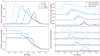 |
Fig. 3. (Left) Evolution of the photon luminosity varying the time tinj for which the injection term is active while keeping the other parameters fixed (though not visually obvious due to the log scale, the total area under each set of curves is the same). The lower panel shows the same curves as the upper one, but with Δt = 0 corresponding to the time of the peak rather than the time of heating onset to more directly compare to the curves displayed in observational studies (see text). (Upper right) Corresponding neutrino luminosity, rescaled for visualisation as in Fig. 2. For clarity, the contribution of the neutrino processes are shown separately only when they are above the quiescence level. (Lower right) Fraction of the total neutrino luminosity coming from the different crustal neutrino reactions that get activated during the outbursts. |
In order to display more clearly the cooling curves, we use as the independent variable the time difference with respect to the beginning of the injection Δt, which is however an information that is not available for observational data. Conversely, to present a cooling curve that is more akin to what can be observed, in the second panel of Fig. 3 we plot the curves computing Δt from the time of the peak (which does not amount to a visual translation when using a log-scale). This operation removes a lot of information and blurs, to an extent, the differences between the lines, demonstrating how new data about the rise phase would be fundamental in constraining tinj.
3.3. Dependence on the injection region geometry
We now consider the effects of the geometry of the heated region on the cooling of the surface hotspot. First, we ran several cases varying the upper injection depth zout, shown in Fig. 4, and the lower one zin, shown in Fig. 5. Overall, these two parameters control the early and late phase of the event, respectively, as the heat diffusion time from to the surface from hot layers increases with their depth.
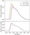 |
Fig. 4. Same of Fig. 3, varying the outermost limit of the heated region zout as reported in the caption, keeping all other parameters fixed, for two envelope models. In this case, the separate contributions are not shown, as they only show marginal differences. |
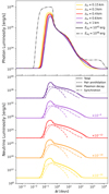 |
Fig. 5. Same as Fig. 3, but varying the inner limit of the injection zin as reported in the caption. In the cases with the largest zin, i.e. with the heating reaching higher density layers, the contribution of two further neutrino emission channels becomes important, namely the emissivity from the formation and breaking of Cooper pairs of superfluid neutrons (e.g. Page et al. 2009) (empty-dotted lines) and the one from n-n and e-ion bremsstrahlung (double dashed lines). |
The outer limit, zout, also strongly affects the peak luminosity: in fact, at lower densities the heat capacity is lower, and a quicker diffusion the radiating surface reduces the amount of energy that is radiated as neutrinos before it can contribute to the luminosity at the surface. In the case of a very shallow injection, zout = 5 m with a realistic hotspot size R = 3 km (see Sect. 3.3), we obtain a peak value Lmax ∼ 1036 erg/s. This is consistent with outburst observations, which show peak luminosities in the 1034 − 1036 erg/s range (Coti Zelati et al. 2018).
Conversely, the inner depth, zin, affects the profile of the outburst at later phases. In particular, as the heat is deposited in denser and denser layers a shoulder appears in the late-time light curve, reflecting an increasing time for heat to diffusively reach the surface. However, this trend seems to be reversed in those cases in which zin is large enough for heat to be deposited underneath the neutron drip point (in our case, located at depth zdrip ≃ 0.8 km), as the shoulder recedes. This is due to the discontinuity of the microphysical properties of the crust at that point, and in particular to the increased specific heat that renders the heat addition in the lower layers less effective. To further assess the effects of this discontinuity, we repeated the simulation with zin = 600 m with a much larger heat input, Einj = 1046 erg, shown as the grey dash-dotted line in Fig. 5. In this case the deeper layers can experience a substantial temperature variation, and the heat emerging from these regions is delayed by the discontinuity in conductivity, forming a plateau-like structure at late times (which also enhances the time before returning to the quiescence luminosity by a substantial factor).
Finally, in Fig. 6 we show the effect of taking a different radius for the injection region. We chose four values for R, namely 1, 2, 3 and 4 km, as the transient blackbody components characterising the spectrum of outbursts have equivalent emission radii of typical length ≲3 km in the early phases, before shrinking during cooling. In the current set-up, the different choices for the initial R yield curves with the same traits, and almost amount to a rescaling of the outburst luminosity, as if it were a geometric effect due to a larger emission surface. It should be noted, however, that this length is related but not equal to the emission radius as obtained from observations, which is affected by general-relativistic ray-bending and the systematics associated with spectral fits. A more detailed study of these effects is deferred to future work. In our runs, we did not observe a marked evolution of the hot region, mainly due to the choice of a polar patch, in which the field lines are almost perpendicular to the surface and thus hinder heat diffusion. However, simulations studied in a 3D set-up (De Grandis et al. 2022) showed that the magnetic field can significantly alter the shape of the hotspot (see Sect. 4).
3.4. The role of the background state: Different stellar masses
Thus far, we considered as a background state a standard 1.4 M⊙ NS. To study the effect of this parameter, in Fig. 7 we compare the evolution of an outburst akin to the one studied in the previous cases (Einj = 1043 erg, tinj = 10 h, R = 3 km, zout = 5 m, zin = 600 m) but for NSs that have masses of 1.2 and 2 solar masses, at the upper and lower end of the values allowed by the EoS. In particular, the latter case allows for fast cooling reactions, which for the BSk24 EoS are allowed above the critical mass MdUrca = 1.595 M⊙. In order to better compare the ensuing cooling curves, we chose two states having the same photon luminosity in quiescence, thus starting the injection at t0 = 42 and 120 kyr, respectively–though, since the evolution of the magnetic field and the corresponding Ohmic heating is not considered, these values do not have a strict physical meaning. The overall shape of the curves is remarkably similar, with several differences in the local slope of the cooling that can be associated with the different neutrino emission channels, becoming dominant at slightly different times, as displayed in the bottom panel. Hence, contrary to what happens for the long term cooling, the mass is not a crucial parameter in the cooling of the hotspot. This is due to the fact that the bulk of the mass, and thus the mass difference, is found in the core, whereas the outburst unfolds within the crust, a region that only has marginal differences in the two cases. The same principle can be applied to different equations of state: whereas the core composition is still very much unknown and varies widely among models, the crustal one is comparatively better understood, and the cooling of a crustal hotspot is not a good proxy for distinguishing between them.
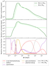 |
Fig. 7. Photon and neutrino luminosity for two cases with heat injection down to z2 = 600 m for two NSs with different masses at the opposite ends of the possible values for NSs. The initial states were chosen in order to have the same quiescence photon luminosity (though the neutrino one is different). In the last panel, the fraction of the total neutrino luminosity due to the active neutrino reactions is displayed. The dominant cooling channel in the quiescence (background state) is different in the two cases, with the more massive star undergoing fast cooling via direct URCA reaction (gray line). |
4. Conclusions
In this work, we presented an updated framework for the description of magnetar outbursts as short-term cooling events. In particular, we studied how the evolution of the luminosity of an outburst can put constraints on the physical parameters characterising the heat injection mechanism, whose precise origin remains elusive to this day.
Our simulations employ a state of the art framework to model the microphysical processes in the crust, alongside a self-consistent treatment of the outer boundary condition for the temperature evolution. Namely, we extended the integration domain of our simulation to include regions of low density, ρ ≈ 107 g cm−3, which required the use of magnetised envelope models that are thinner than what normally used in cooling simulations as a boundary condition. They can thus be used to study shorter timescales without breaking the plane-parallel approximation. With this set-up, we could obtain the peak luminosity values observed in magnetars in outburst, ≲1036 erg/s, from a heated patch having a realistic emission radius (≲3 km). This result holds even when using envelope models with different chemical compositions (i.e. not just in a light-element scenario), which actually turns out not to be a crucial parameter, as neutrino emission is the limiting factor of the maximum luminosity achievable.
We studied the effect of several parameters related to the initial shape of the heated region, finding an overall similar behaviour, especially in terms of the total timescale of the event. On the other hand, many factors determine the specific features in the shape of the cooling curve. The initial depth of the heat deposition tracks the heat diffusion time up to the surface, and the slope of the photon luminosity curve acts as an indicator of the weak processes dominating the neutrino emission at a given time.
In order to account for the observed luminosity, we find that at least some part of the heating should happen in the very shallow layers of the crust (ρ ≲ 108 g cm−3), leaving open both the possibilities of an internal release at low density or a magnetospheric origin. On the other hand, constraints on the maximum depth that the heat can reach (or originate from) may come from the study of the late phases of the outbursts, when the hot spot has cooled down considerably. Still, most magnetars are already quite hot in their quiescence state (≳1033 erg/s), so that the cooling of the hotspot in the late phases may be difficult to detect against the background emission. This makes highlights the importance to study the so-called low-field magnetars, a small class of objects that shows magnetar-like outbursts while at the same time exhibiting luminosity and spin-down field values akin to those of ordinary pulsars (Rea et al. 2010, 2012). A continued monitoring of the cooling of their outbursts well after the peak, even for several years, may prove key to constraining the depth at which heat is liberated when the outburst is triggered, and hence the heating mechanism itself. However, the small number of these sources and the difficulties inherent in gathering long-exposure data data of dim sources that require long exposure times makes such detailed studies rather challenging.
Another factor rendering low-field magnetars particularly interesting is that they are expected to actually host ultra-strong fields, as strong as ≈1016 G, in small-scale structure and/or a strong toroidal component buried under their surface (e.g. Turolla et al. 2011; Tiengo et al. 2013; Igoshev et al. 2025). This could give rise to extremely large heat depositions, which, as in the case shown in Fig. 5, could display characteristic late-time features.
The timescale over which the heating mechanism operates is another quantity that manifests itself directly in the shape of the luminosity curve, as it is well traced by the delay between the trigger and the onset of the luminosity descent. However, this implies that in order to characterise this parameter it would be necessary to have data about the outburst rise phase, or at the very least a stringent limit on its duration. Unfortunately, no information of this kind is currently available. New missions such as Einstein Probe (Yuan et al. 2025) monitoring the X-ray sky with high cadence and sensitivity are going to provide fundamental information in the upcoming years, with the potential of putting the most stringent constraints to date to the trigger mechanism.
A key aspect of magnetar outbursts that we could not explore in the present study is how different magnetic field strengths and configurations affect the evolution of the event. We did test other field configurations, including some with several multipolar components structures as well as core-threading structures (as in Akgün et al. 2013), but found no significant difference with respect to the runs presented in this work. This is because the luminosity curves in the current 2D set-up are affected by the field in the proximity of the pole and in the outer layers, where the deviation from a dipole cannot be but marginal in axial symmetry. Much in the same way, we tested different magnetar-like fields strengths without finding substantial differences with respect to the runs at 1014 G presented above. Nevertheless, the field structure has been shown to be a crucial factor using 3D codes: in particular, De Grandis et al. (2022) showed that if the heat is injected in a region where the field has a large component parallel to the surface (in contrast to the polar region considered in this work) the duration of the cooling phase can increase significantly due to the additional magnetic insulation. This may explain the prolonged enhanced brightness of some sources, such as SGR J1745−2900 (the so-called Galactic centre magnetar, Rea et al. 2020). Moreover, the evolution of the field may play a role even on smaller timescales; for example in case of the presence of local instabilities (possibly related to the outburst trigger) or thermo-magnetic effects related to the large temperature gradient between the hotspot and the rest of the crust (e.g. Gakis & Gourgouliatos 2024). We defer the study of these effects to future work, employing a 3D code informed by our present 2D results.
Furthermore, in this work we restricted ourselves to the study of integrated quantities, rather than addressing the evolution of the observed spectral parameters, such as temperature and radius of the hotspot. This is due to the fact that these values are affected not only by the cooling of the hotspot itself, but also by other factors like the viewing geometry of the star, general relativistic effects, interstellar absorption and instrumental biases (e.g. Viganò et al. 2014). The study of these parameters and how this information can open new windows in constraining the geometry of the surface of a magnetar will be addressed in future work.
The expression for this emissivity contribution used here is the one proposed by Itoh et al. (1996), which does not take into account the effect of the magnetic field, for simplicity of implementation. We tested as an alternative the one proposed in Yakovlev et al. (2001), finding an analogous behaviour; still, the literature lacks more modern, magnetised calculations.
Acknowledgments
We thank A. Yu. Potekhin for discussion. DDG is supported by a Juan de la Cierva fellowship (JDC2023-052264-I). DDG and NR are supported by the European Research Council (ERC) via the Consolidator Grant ‘MAGNESIA’ (No. 817661) and the Proof of Concept ‘DeepSpacePulse’ (No. 101189496). DDG, NR and KK are supported by the Catalan grant SGR2021-01269 (PI: Graber/Rea), and by the program Unidad de Excelencia Maria de Maeztu CEX2020-001058-M.6953. FCZ is supported by a Ramón y Cajal fellowship (grant650 agreement RYC2021-030888-I). Part of the simulations presented in this paper have been operated in collaboration with the Port d’Informació Científica (PIC) data center. PIC is maintained through a collaboration agreement between the Institut de Física d’Altes Energies (IFAE) and the Centro de Investigaciones Energéticas, Medioambientales y Tecnológicas (CIEMAT).
References
- Aguilera, D. N., Pons, J. A., & Miralles, J. A. 2008, A&A, 486, 255 [NASA ADS] [CrossRef] [EDP Sciences] [Google Scholar]
- Akgün, T., Reisenegger, A., Mastrano, A., & Marchant, P. 2013, MNRAS, 433, 2445 [Google Scholar]
- Ascenzi, S., Viganò, D., Dehman, C., et al. 2024, MNRAS, 533, 201 [NASA ADS] [CrossRef] [Google Scholar]
- Beloborodov, A. M. 2009, ApJ, 703, 1044 [NASA ADS] [CrossRef] [Google Scholar]
- Bernardini, F., Israel, G. L., Stella, L., et al. 2011, A&A, 529, A19 [NASA ADS] [CrossRef] [EDP Sciences] [Google Scholar]
- Beznogov, M. V., Potekhin, A. Y., & Yakovlev, D. G. 2021, Phys. Rep., 919, 1 [CrossRef] [Google Scholar]
- Bochenek, C. D., Ravi, V., Belov, K. V., et al. 2020, Nature, 587, 59 [NASA ADS] [CrossRef] [Google Scholar]
- Borghese, A., Rea, N., Turolla, R., et al. 2019, MNRAS, 484, 2931 [NASA ADS] [CrossRef] [Google Scholar]
- Borghese, A., Rea, N., Turolla, R., et al. 2021, MNRAS, 504, 5244 [NASA ADS] [CrossRef] [Google Scholar]
- Caleb, M., & Keane, E. 2021, Universe, 7, 453 [NASA ADS] [CrossRef] [Google Scholar]
- Carrasco, F., Viganò, D., Palenzuela, C., & Pons, J. A. 2019, MNRAS, 484, L124 [Google Scholar]
- CHIME/FRB Collaboration (Andersen, B. C., et al.) 2020, Nature, 587, 54 [Google Scholar]
- Coti Zelati, F., Rea, N., Pons, J. A., Campana, S., & Esposito, P. 2018, MNRAS, 474, 961 [NASA ADS] [CrossRef] [Google Scholar]
- Coti Zelati, F., Borghese, A., Rea, N., et al. 2020, A&A, 633, A31 [NASA ADS] [CrossRef] [EDP Sciences] [Google Scholar]
- De Grandis, D., Turolla, R., Taverna, R., et al. 2022, ApJ, 936, 99 [Google Scholar]
- Dehman, C., Viganò, D., Rea, N., et al. 2020, ApJ, 902, L32 [NASA ADS] [CrossRef] [Google Scholar]
- Dehman, C., Viganò, D., Pons, J. A., & Rea, N. 2023, MNRAS, 518, 1222 [Google Scholar]
- Deibel, A., Cumming, A., Brown, E. F., & Reddy, S. 2017, ApJ, 839, 95 [Google Scholar]
- Duncan, R. C., & Thompson, C. 1992, ApJ, 392, L9 [Google Scholar]
- Esposito, P., Israel, G. L., Zane, S., et al. 2008, MNRAS, 390, L34 [NASA ADS] [Google Scholar]
- Esposito, P., Rea, N., & Israel, G. L. 2021, Astrophys. Space Sci. Lib., 461, 97 [NASA ADS] [CrossRef] [Google Scholar]
- Gakis, D., & Gourgouliatos, K. N. 2024, A&A, 690, A117 [NASA ADS] [CrossRef] [EDP Sciences] [Google Scholar]
- Gavriil, F. P., Kaspi, V. M., & Woods, P. M. 2004, ApJ, 607, 959 [Google Scholar]
- Gourgouliatos, K. N., & Pons, J. A. 2019, Phys. Rev. Res., 1, 032049 [Google Scholar]
- Gudmundsson, E. H., Pethick, C. J., & Epstein, R. I. 1983, ApJ, 272, 286 [CrossRef] [Google Scholar]
- Ibrahim, A. Y., Borghese, A., Coti Zelati, F., et al. 2024, ApJ, 965, 87 [Google Scholar]
- Igoshev, A., Barrère, P., Raynaud, R., et al. 2025, Nat. Astron., 9, 541 [Google Scholar]
- Israel, G. L., Esposito, P., Rea, N., et al. 2016, MNRAS, 457, 3448 [NASA ADS] [CrossRef] [Google Scholar]
- Itoh, N., Hayashi, H., Nishikawa, A., & Kohyama, Y. 1996, ApJS, 102, 411 [NASA ADS] [CrossRef] [Google Scholar]
- Kaspi, V. M., & Beloborodov, A. M. 2017, ARA&A, 55, 261 [Google Scholar]
- Kennea, J. A., Burrows, D. N., Kouveliotou, C., et al. 2013, ApJ, 770, L24 [Google Scholar]
- Kovlakas, K., De Grandis, D., & Rea, N. 2025, A&A, in press, https://doi.org/10.1051/0004-6361/202554742 [Google Scholar]
- Lander, S. K. 2023, ApJ, 947, L16 [Google Scholar]
- Li, X., Levin, Y., & Beloborodov, A. M. 2016, ApJ, 833, 189 [NASA ADS] [CrossRef] [Google Scholar]
- Mereghetti, S., Götz, D., Weidenspointner, G., et al. 2009, ApJ, 696, L74 [NASA ADS] [CrossRef] [Google Scholar]
- Mereghetti, S., Pons, J. A., & Melatos, A. 2015, Space Sci. Rev., 191, 315 [NASA ADS] [CrossRef] [Google Scholar]
- Mereghetti, S., Savchenko, V., Ferrigno, C., et al. 2020, ApJ, 898, L29 [Google Scholar]
- Muno, M., Gaensler, B., Clark, J. S., et al. 2006, ATel, 902, 1 [Google Scholar]
- Muno, M. P., Gaensler, B. M., Clark, J. S., et al. 2007, MNRAS, 378, L44 [NASA ADS] [Google Scholar]
- Page, D., Lattimer, J. M., Prakash, M., & Steiner, A. W. 2004, ApJS, 155, 623 [NASA ADS] [CrossRef] [Google Scholar]
- Page, D., Lattimer, J. M., Prakash, M., & Steiner, A. W. 2009, ApJ, 707, 1131 [Google Scholar]
- Pearson, J. M., Chamel, N., Potekhin, A. Y., et al. 2019, MNRAS, 486, 768 [NASA ADS] [CrossRef] [Google Scholar]
- Petroff, E., Hessels, J. W. T., & Lorimer, D. R. 2022, A&ARv, 30, 2 [NASA ADS] [CrossRef] [Google Scholar]
- Pons, J. A., & Rea, N. 2012, ApJ, 750, L6 [NASA ADS] [CrossRef] [Google Scholar]
- Potekhin, A. Y., Chabrier, G., & Yakovlev, D. G. 2007, Ap&SS, 308, 353 [Google Scholar]
- Potekhin, A. Y., Pons, J. A., & Page, D. 2015, Space Sci. Rev., 191, 239 [Google Scholar]
- Rea, N., & Esposito, P. 2011, Astrophys. Space Sci. Proc., 21, 247 [NASA ADS] [CrossRef] [Google Scholar]
- Rea, N., Esposito, P., Turolla, R., et al. 2010, Science, 330, 944 [NASA ADS] [CrossRef] [Google Scholar]
- Rea, N., Israel, G. L., Esposito, P., et al. 2012, ApJ, 754, 27 [NASA ADS] [CrossRef] [Google Scholar]
- Rea, N., Coti Zelati, F., Viganò, D., et al. 2020, ApJ, 894, 159 [CrossRef] [Google Scholar]
- Sridhar, N., Metzger, B. D., Beniamini, P., et al. 2021, ApJ, 917, 13 [NASA ADS] [CrossRef] [Google Scholar]
- Thorne, K. S. 1977, ApJ, 212, 825 [NASA ADS] [CrossRef] [Google Scholar]
- Tiengo, A., Esposito, P., Mereghetti, S., et al. 2013, Nature, 500, 312 [CrossRef] [Google Scholar]
- Turolla, R., Zane, S., Pons, J. A., Esposito, P., & Rea, N. 2011, ApJ, 740, 105 [NASA ADS] [CrossRef] [Google Scholar]
- Turolla, R., Zane, S., & Watts, A. L. 2015, Rep. Prog. Phys., 78, 116901 [Google Scholar]
- Typel, S., Oertel, M., & Klähn, T. 2015, Phys. Part. Nucl., 46, 633 [CrossRef] [Google Scholar]
- van der Horst, A. J., Connaughton, V., Kouveliotou, C., et al. 2010, ApJ, 711, L1 [Google Scholar]
- Viganò, D., Perna, R., Rea, N., & Pons, J. A. 2014, MNRAS, 443, 31 [CrossRef] [Google Scholar]
- Viganò, D., Garcia-Garcia, A., Pons, J. A., Dehman, C., & Graber, V. 2021, Comp. Phys. Commun., 265, 108001 [Google Scholar]
- Yakovlev, D. G., Kaminker, A. D., Gnedin, O. Y., & Haensel, P. 2001, Phys. Rep., 354, 1 [NASA ADS] [CrossRef] [Google Scholar]
- Younes, G., Kouveliotou, C., Jaodand, A., et al. 2017, ApJ, 847, 85 [NASA ADS] [CrossRef] [Google Scholar]
- Younes, G., Güver, T., Kouveliotou, C., et al. 2020, ApJ, 904, L21 [CrossRef] [Google Scholar]
- Yuan, W., Dai, L., Feng, H., et al. 2025, Sci. China: Phys. Mech. Astron., 68, 239501 [Google Scholar]
All Figures
|
Fig. 1. Tb–Ts relations calculated for a sample of representative values of Ts in the case of Fe envelopes. Different colours and markers denote different bottom-of-the-envelope densities ρb. The models from Gudmundsson et al. (1983) and Potekhin et al. (2015), calculated for the standard value ρb = 1010 g cm−3, are plotted for reference. The spread of the points at the same Ts (which is noticeable only in the bottom panel) corresponds to different ΘB, with higher Tb giving a lower Ts value for the same Tb. Two values for the magnetic field, 108 G (top panel) and 1012 G (bottom panel) are shown; these values have been chosen, although comparatively low, for clarity of visualisation, as stronger fields yield very sparse plots. |
| In the text | |
|
Fig. 2. (Top panel) Photon luminosity with growing heat injection, in the case of Fe (solid lines) or H (dashed lines) envelopes. (Bottom panel) Corresponding neutrino luminosity, with its dominant channels: a continuous line indicates the total Lν, dashed lines the contribution from e+e− pair annihilation, dotted lines the one from plasmon decay, and the dash-dotted the weak-synchrotron emission. The baseline of neutrino luminosity, not plotted separately, is in this case due to the breaking of 2P2 Cooper pairs in the core. For clarity of presentation, we rescaled each family of curves by a factor indicated in the figure, and only the curves calculated with the H envelope are displayed (the ones corresponding to the Fe envelope are almost indistinguishable from them). |
| In the text | |
|
Fig. 3. (Left) Evolution of the photon luminosity varying the time tinj for which the injection term is active while keeping the other parameters fixed (though not visually obvious due to the log scale, the total area under each set of curves is the same). The lower panel shows the same curves as the upper one, but with Δt = 0 corresponding to the time of the peak rather than the time of heating onset to more directly compare to the curves displayed in observational studies (see text). (Upper right) Corresponding neutrino luminosity, rescaled for visualisation as in Fig. 2. For clarity, the contribution of the neutrino processes are shown separately only when they are above the quiescence level. (Lower right) Fraction of the total neutrino luminosity coming from the different crustal neutrino reactions that get activated during the outbursts. |
| In the text | |
|
Fig. 4. Same of Fig. 3, varying the outermost limit of the heated region zout as reported in the caption, keeping all other parameters fixed, for two envelope models. In this case, the separate contributions are not shown, as they only show marginal differences. |
| In the text | |
|
Fig. 5. Same as Fig. 3, but varying the inner limit of the injection zin as reported in the caption. In the cases with the largest zin, i.e. with the heating reaching higher density layers, the contribution of two further neutrino emission channels becomes important, namely the emissivity from the formation and breaking of Cooper pairs of superfluid neutrons (e.g. Page et al. 2009) (empty-dotted lines) and the one from n-n and e-ion bremsstrahlung (double dashed lines). |
| In the text | |
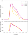 |
Fig. 6. Same as Fig. 3 varying the radius of the heated region R. |
| In the text | |
|
Fig. 7. Photon and neutrino luminosity for two cases with heat injection down to z2 = 600 m for two NSs with different masses at the opposite ends of the possible values for NSs. The initial states were chosen in order to have the same quiescence photon luminosity (though the neutrino one is different). In the last panel, the fraction of the total neutrino luminosity due to the active neutrino reactions is displayed. The dominant cooling channel in the quiescence (background state) is different in the two cases, with the more massive star undergoing fast cooling via direct URCA reaction (gray line). |
| In the text | |
Current usage metrics show cumulative count of Article Views (full-text article views including HTML views, PDF and ePub downloads, according to the available data) and Abstracts Views on Vision4Press platform.
Data correspond to usage on the plateform after 2015. The current usage metrics is available 48-96 hours after online publication and is updated daily on week days.
Initial download of the metrics may take a while.