| Issue |
A&A
Volume 701, September 2025
|
|
|---|---|---|
| Article Number | A69 | |
| Number of page(s) | 9 | |
| Section | Astrophysical processes | |
| DOI | https://doi.org/10.1051/0004-6361/202555222 | |
| Published online | 04 September 2025 | |
Polarized, variable radio emission from the scallop-shell binary system DG CVn
1
Institut de Ciències de I’Espai (ICE-CSIC), Campus UAB, Carrer de Can Magrans s/n, 08193 Cerdanyola del Vallès, Catalonia, Spain
2
Institut d’Estudis Espacials de Catalunya (IEEC), 08860 Castelldefels, Barcelona, Catalonia, Spain
3
Institute of Applied Computing & Community Code (IAC3), University of the Balearic Islands, Palma, 07122
Spain
4
Department of Physics & Astronomy, Bucknell University, Lewisburg, PA, USA
5
Instituto de Astrofísica de Canarias (IAC), 38205 La Laguna, Tenerife, Spain
6
Departamento de Astrofísica, Universidad de La Laguna (ULL), 38206 La Laguna, Tenerife, Spain
7
Centre for Planetary Habitability, Department of Geosciences, University of Oslo, Sem Saelands vei 2b, 0315 Oslo, Norway
8
Institut für Astrophysik, Georg-August-Universität, Friedrich-Hund-Platz 1, 37077 Göttingen, Germany
9
Observatories of the Carnegie Institution for Science, Pasadena, CA, 91101
USA
10
ASTRON, Netherlands Institute for Radio Astronomy, Oude Hoogeveensedijk 4, Dwingeloo, 7991 PD
The Netherlands
11
Instituto de Astrofísica de Andalucía (IAA-CSIC), Glorieta de la Astronomía s/n, E-18008 Granada, Spain
12
Center for Astroparticles and High Energy Physics (CAPA), Universidad de Zaragoza, E-50009 Zaragoza, Spain
13
School of Sciences, European University Cyprus, Diogenes street, Engomi, 1516 Nicosia, Cyprus
⋆ Corresponding author: This email address is being protected from spambots. You need JavaScript enabled to view it.
Received:
19
April
2025
Accepted:
11
July
2025
Abstract
DG CVn is an eruptive variable star and represents the closest member of the known sample of complex periodic variables, or scallop-shell stars. Over the years, this M dwarf binary system has shown significant flaring activity at a wide range of frequencies. Here, we present a detailed analysis of ∼14 hours of radio observations of this stellar system, taken with the Karl G. Jansky Very Large Array at band L, centered at 1.5 GHz. In both 7-hour-long observations we have found a quiescent, weakly polarized component that could be ascribable to the incoherent, gyro-synchrotron emission coming from the magnetosphere surrounding one or both stars, along with multiple ∼90% right-circularly polarized bursts, some of which last for a few minutes and others of which last longer, ≳30 minutes Some of these bursts show a drift in frequency and time, possibly caused due to beaming effects or the motion of the plasma responsible for the emission. We assess the possible modulation of burst frequency with the primary and secondary periods, and discuss the properties of these bursts, favoring electron cyclotron maser over plasma emission as the likely underlying mechanism. We compare DG CVn’s dynamic spectrum to other young M dwarfs and find many similarities. A proper, dedicated, simultaneous radio/optical follow-up is needed to monitor the long-term variability and increase the statistics of bursts, in order to test whether the corotating absorbers detected in the optical can drive the observed radio emission, and whether the occurrence of radio bursts correlates with the rotational phase of either star.
Key words: binaries: visual / stars: flare / stars: low-mass / stars: magnetic field / stars: rotation
© The Authors 2025
 Open Access article, published by EDP Sciences, under the terms of the Creative Commons Attribution License (https://creativecommons.org/licenses/by/4.0), which permits unrestricted use, distribution, and reproduction in any medium, provided the original work is properly cited.
This article is published in open access under the Subscribe to Open model. This email address is being protected from spambots. You need JavaScript enabled to view it. to support open access publication.
1. Introduction
M dwarfs are the most abundant stars in the Galaxy (Chabrier 2001; Henry et al. 2006) and are frequently characterized by their strong magnetic fields, typically hundreds to thousands of gauss (Reiners et al. 2022), along with recurrent flaring activity observed across the electromagnetic spectrum from radio waves to X-rays (Villadsen & Hallinan 2019; Joseph et al. 2024). Several surveys indicate that mid-to-late M dwarfs flare with remarkable frequency, with over 40% of stars of spectral type M4 or later exhibiting detectable flares, which is over an order of magnitude higher than what is observed in Sun-like stars (Günther et al. 2020; Yiu et al. 2024).
The recent advancements in radio astronomy and several wide radio surveys have unveiled a growing, yet still very small, fraction of main-sequence stars that are radio-loud (Yiu et al. 2024; Driessen et al. 2024). Most of them are chromospherically active M dwarfs, and/or interacting binary systems. In M dwarfs, radio emission can generally be put into two categories. The first one is an apparently steady (quiescent) component that is relatively weak, often non- or weakly polarized, and broadband, similar to solar microwave flares (Dulk 1985; Alissandrakis 1986; Yiu et al. 2024); it can typically be ascribed to incoherent gyro-synchrotron radiation. The second class comprises transient events, which are the intense flare-associated bursts characterized by narrow bandwidths, high brightness temperatures (often TB ≫ 1012 K), and strong circular polarization (Dulk 1985; Melrose & Dulk 1982; Melrose 2017). These are thought to be produced by two possible coherent emission mechanisms: plasma emission and electron cyclotron maser (ECM). The latter may be driven by aurora-like current systems in stellar magnetospheres similar to what is seen in ultracool dwarfs (McLean et al. 2011; Kaur et al. 2024; Bloot et al. 2024), and is responsible for Jupiter’s intense decametric radio emissions (Farrell et al. 1999; Zarka 2004).
Radio bursts are of specific interest because they offer a unique window into the underlying magnetic fields and particle acceleration mechanisms, providing deeper insights into the energetic processes that drive their dynamic stellar environments (McLean et al. 2011; Villadsen & Hallinan 2019; Bloot et al. 2024; Kaur et al. 2024; Kavanagh et al. 2024). Notably, some M dwarfs are known to show periodic, pulse-like radio flares that are related to the star’s rotation period. Two striking examples of this behavior are UV Cet (Zic et al. 2019) and AU Mic (Bloot et al. 2024), both with very high circular polarization. AD Leo is another nearby flare star, which emits with variability over different timescales, as short as milliseconds (Zhang et al. 2023).
In this paper, we study DG CVn, also cataloged as TIC 368129164 in TESS, and GJ 3789. Its SIMBAD coordinates are RAJ2000 = 13h31m46.6s and δJ2000 = +29° 16′36.7″, and it exhibits a high proper motion of μRA = −242.8 ± 0.5 mas yr−1 and μδ = −149.8 ± 0.3 mas yr−1 (Gaia Collaboration 2021). Further, DG CVn forms a visual binary of two M4 V components with a projected separation of ∼0.2″ (i.e., a few astronomical units). It is a well-known eruptive variable (Beuzit et al. 2004; Cortés-Contreras et al. 2017; Helfand et al. 1999), and the Swift satellite detected a gamma-ray super flare from it in 2014 (Osten et al. 2016), followed by two bright (∼100 mJy) radio flares at 15 GHz, among the most luminous incoherent radio flares ever observed from a red dwarf star, before it returned to a quiescent level of 2–3 mJy after ∼4 days (Fender et al. 2015). The target has also been detected at lower frequencies in the LOFAR, VLASS, and ASKAP surveys (Yiu et al. 2024; Driessen et al. 2024) (see Sect. 3.3), but those snapshot observations did not reveal whether the emission is burst-like or quiescent.
At a reported distance of d = 18 pc, DG CVn is also the closest confirmed scallop-shell star (SSS), also known as complex periodic variables. These are a newly identified class of objects characterized by multiple oddly shaped dips in their optical light curve. This suggests the presence of opaque corotating material that could either be gas from the star trapped in huge prominences, or dust coming from the disk debris or an out-gassing rocky planet (Bouma et al. 2024; Stauffer et al. 2017; Zhan et al. 2019; Koen 2021; Waugh & Jardine 2022). Like all SSSs, DG CVn is a young system, with several age diagnostics pointing at an age between 40–150 Myr, depending on its possible association with the Carina–Columba complex (Riedel et al. 2014) or the AB Doradus moving group (Bell et al. 2015). Its fast rotation indicates that it probably has an age younger than 150 Myr, too (Engle & Guinan 2023). In the TESS-based catalog of SSSs by Bouma et al. (2024), DG CVn shows photometric periods of a few hours: P1 = 6.44 h and P2 = 2.60 h, possibly interpreted as the rotational period of the two stars (Bouma et al. 2024). Such periodicity is consistently seen in different TESS sectors, meaning that it is stable over several years at least, although the morphology of the dips substantially changes (see Appendix A for the TESS light curves of DG CVn and a short discussion).
Radio observations can cast a light on the enigma by distinguishing if the radio emission is a counterpart of the stochastic chromospheric activity commonly seen in young, fast-rotating M dwarfs, or auroral emission either associated with fast rotation or caused by magnetic interaction with the occulting material. For instance, centrifugal breakout of corotating clumps has been considered as a possible mechanism even for non-SSS stars such as UV Cet (Bastian et al. 2022). A cross-matching of the most complete SSS sample (Bouma et al. 2024) with the recent radio-star catalogs based on VLASS, LoTSS, and ASKAP-RACS surveys (Yiu et al. 2024; Driessen et al. 2024) suggests that there are currently few more known radio-loud SSSs. The (biased) observed radio occurrence of SSS is in line with the sample of young M dwarfs, and is likely a combination of sporadicity of transient radio bursts, limited observational coverage, and low quiescent radio luminosity. In this context, the only two SSSs with dedicated, long radio observations, as far as we know, are: DG CVn, presented in this study, and 2MASS J05082729−2101444 (J0508-21) with the upgraded Giant Metrewave Radio Telescope at 575–720 MHz, presented by Kaur et al. (2024), who proposed evidence of coherent radio auroral emission and discussed whether the radio and optical behavior could ultimately be powered by the same orbiting material. In this context, exploring the radio behavior of SSSs like J0508-21 and DG CVn, along with well-coordinated photometric campaigns, could help shed light on the physics responsible for this poorly understood type of young low-mass stellar systems.
In this article, we present a detailed analysis of 14 hours of archival (2018) observations of DG CVn with Karl G. Jansky Very Large Array (VLA) at band L (1–2 GHz). In Sect. 2, we describe the VLA observations and the data analysis. In Sect. 3, we present the results, discussing the dynamic spectrum morphology and possible periodic variability, and compare the results to other M dwarfs in Sect. 4.
2. VLA observations and data reduction
The target DG CVn was observed at band L (1–2 GHz), as part of the VLA proposal 17B-370 (PI: J. Villadsen), on January 21st (configuration B) and February 20th, 2018 (BnA), covering ∼6 hours on the target in both epochs (the second observation was split by a gap of ∼1 hour). For both observations, 3C286 was observed as the standard flux calibrator, while J1330+2509 served as the gain calibrator. The observations were performed in continuum standard mode with 16 spectral windows, each having a bandwidth of 64 MHz, and 64 (1-MHz wide) channels.
The entire dataset underwent processing via Common Astronomy Software Applications (CASA; CASA Team 2022). The calibration of the data adheres to the standard CASA VLA pipeline. For VLA band L, both Stokes V and I are formed from the parallel-hand correlation products, RR and LL, with Stokes I = (LL+RR)/2 and Stokes V = (RR-LL)/2. The observations did not include polarization calibrators. Therefore, we did not perform linear polarization measurements from the crosshand products, RL and LR. After an additional round of manual flagging to correct for the remaining bad data, the maps were constructed with the CASA task tclean by using the standard gridding algorithm and employing a natural weighting scheme across all image planes. Further, we used the Cube Analysis and Rendering Tool for Astronomy (CARTA; Ott et al. 2022; Comrie et al. 2021) for image visualization.
We used CASA task imfit to extract the flux statistics from the image plane for the LL and RR correlations, and the Stokes I and V parameters. We summarize these flux statistics in Table 1. We applied the same approach to examine the time variability in flux from the image plane by making clean maps for every 5-minute scan on the target.
VLA band L observations.
To build the dynamic spectrum, we shifted the phase center to the position of our source, averaged the data over all baselines, and made use of CASA task visstat to compute the statistics for the real part of the amplitude from the visibility plane. It computes the statistics for the RR and LL correlators separately. From these statistics, we evaluated the Stokes V component as (RR-LL)/2, following the standard IAU convention. In a dataset in which there are no bright background sources, the real part of the amplitude gives a fair estimate of the flux at the phase center, while the imaginary component of the amplitude reflects the noise level (see e.g., Villadsen & Hallinan 2019 for more discussion). The analysis of the dynamic spectrum allowed us to infer the flux variability for even shorter time bins and for every frequency channel, allowing us to uncover the presence of relatively bright bursts. As we are particularly interested in coherent, highly circularly polarized bursts, we did not perform additional subtraction of the background sources, as there were no nearby sources brighter than the target in Stokes V in the field of view that could possibly have contaminated the emission at the phase center.
3. Results
The VLA L-band emission in both circular components (LL and RR) is detected in the two epochs (see Fig. 1). The observed radio position is compatible with the previously reported values for DG CVn once we correct for Gaia DR2 proper motion given in Sect. 1. Table 1 summarizes the main characteristics of the observations and the flux statistics of the January, February, and January+February observations. In all cases, the peak and integrated fluxes are compatible with each other, indicating that the source is unresolved. From January to February, the average Stokes I and V fluxes decrease by a factor of ∼1.5 and ∼3 in Stokes I and V, respectively. This change is actually related to the presence of bursts with different energetics, rather than a variation in the quiescent emission, as is shown in the next subsection.
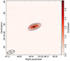 |
Fig. 1. Combined map for the January and February observations, centered at the emission peak, which shows an offset from the SIMBAD position that is compatible with the reported proper motion of DG CVn. The synthesized beam is shown in the lower left corner and the cross (+) marks the proper motion corrected position. The color scale represents the Stokes I flux density, while the contours indicate the Stokes V signal, corresponding to levels of 5, 10, 20, 30, 40, and 50 σrmsV (where σrmsV is ∼11.2 μJy/beam). |
3.1. Time variability
We took advantage of the high S/N ratio of the Stokes V emission to investigate variability on short timescales. Figure 2 shows the 5-minute binned light curves, which are phase-folded with the primary and secondary photometric periods, P1 = 6.44 h and P2 = 2.60 h (Bouma et al. 2024), and we define the corresponding phases as Φ1 and Φ2. Hereafter, we arbitrarily set the reference phase ϕ1, 2 = 0 at the beginning of the first target scan of the January observation (21 January, 2018, at 07:17:00 UT). Both in January and February, the LL component remains compatible with being constant and never exceeds the RR component. The latter, instead, varies on different timescales, showing several ∼10 − 45 minute-long bursts. During these bursts, the intensity is enhanced up to one order of magnitude, and the net circular polarization fraction can become very high, up to ∼90%. If we consider the total time period during which the source shows an RR excess over the total 11.8 hours of on-source time, the source appears to have a burst duty cycle of ∼15%.
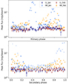 |
Fig. 2. Phase-aligned light curves for LL and RR correlations using the primary period P1 = 6.44 h (top) and the secondary period P2 = 2.60 h (bottom), reported in Bouma et al. (2024). The flux represents the peak flux values on a logarithmic scale extracted from the image planes of each 5-minute scan, using the CASA task imfit. Here, phase |

From Fig. 2, we note that when folded with P1, the emission is quiescent in the phase range Φ1 ≃ 0.90 − 0.35, while bursts are scattered and occur at various phases. Unfortunately, the February observations contain a gap precisely at the phases where the main January burst occurred, preventing us from confirming whether bursts repeat around Φ1 ∼ 0.4 in February. On the other hand, when folded with the secondary period, P2, the RR excess appears to cluster around the phase range Φ2 ∼ 0.8 − 0.2.
We refer to Appendix A for a brief illustration of the TESS light curves, although a dedicated multi-instrument photometric campaign is ongoing and will be the subject of a dedicated study with more in-depth discussion. As far as this study of radio behavior is concerned, it is important to note that the optical modulation with P2 is sinusoidal, meaning that the SSS behavior (i.e., presence of dips) is likely related to P1 only. If confirmed by future observations, and if we assume that the two periods reflect the spins of the two stars, this would suggest that these radio bursts may cluster with the rotational phase of the faster rotator of the binary, and would not be related to the dips, which appear with periodicity P1. On the other hand, there appears a subtle suggestion that the duration of the most complex bursts is roughly comparable to the duration of the dips.
A possible clustering with the photometric phase has possibly also been observed in J0508-21, the other SSS for which radio light curves have been studied (at 0.55–0.75 GHz, Kaur et al. 2024). However, in both cases, additional data is required to advance a claim with sound statistical evidence (as Bloot et al. 2024 did for the rotational clustering of radio bursts in AU Mic). Moreover, note that in our case we cannot put the TESS and radio light curves in phase, since they are separated by more than 2 years at least, a timescale over which the morphology of the dips is seen to drastically change, and over which the accumulated ephemeris errors make it impossible to maintain the phase coherence (see Appendix A for a short discussion).
3.2. Dynamic spectra
In Fig. 3, we show the dynamic spectra for Stokes V, generated using the methodology explained in Sect. 2, with a time sampling of 60 seconds and a frequency resolution of 16 MHz. For the January observations, the dynamic spectrum shows the presence of three distinct right-hand circularly polarized (RCP) radio bursts, distributed across different time intervals within the seven-hour observing window. The first burst is the most intense, exhibiting a polarization fraction of almost 90% with the RCP flux reaching over 25 mJy. The analysis of the dynamic spectrum reveals that this burst persists for ∼45 minutes Several fine-scale structures are also evident, including two secondary peaks embedded within the broader burst profile. Specifically, the flux initially increases, followed by a temporary decline, before rising again to form a secondary peak. It subsequently reaches its major peak, followed by a rapid decline into the quiescent phase. During the rising phase of this burst, the emission is predominantly concentrated at the lower frequency range of the L band, whereas during its peak phase the flux intensity is more pronounced at the higher end of the L band.
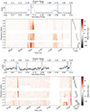 |
Fig. 3. Dynamic spectra for Stokes V for January (top) and February (bottom) observations, taken from visibility plane. The error bars in the light curves and frequency spectrum represent the standard deviation, computed by considering the imaginary component of the amplitude. The top and bottom axes of the top panel represent the primary and secondary phases (Φ1 and Φ2), respectively, calculated using the primary and secondary periods reported in Bouma et al. (2024). We fixed the reference phase Φ = 0 at the beginning of the first target scan in the January observation. The vertical blue lines indicate the start (Φ = 0) of new primary (dashed) and secondary (solid) cycles, respectively. |
The second burst of the January observation occurs nearly two hours after the first one and exhibits a lower flux density, with a peak RCP flux of ∼15 mJy. This event has a duration of ∼30 minutes and is spectrally broad. Throughout its entire duration, the emission is most prominent at the lower end of the L band. The third burst is detected approximately 30 minutes after the decay of the second burst and is the faintest among the three. It has a relatively short duration, lasting only a few minutes. Unlike the first two bursts, this event is brightest in the central portion of the L band (between 1.2 and 1.5 GHz) and shows clear evidence of a frequency drift.
During the first session of the February observations, which lasted 5.5 hours, an RCP flare was detected, with a duration of no more than 10 minutes When phase-folded with P2 (Bouma et al. 2024), this flare partially overlaps with the third flare observed in January, occurring around phase Φ2 ∼ 0.1. This burst also exhibits a clear frequency drift and appears to follow a preceding faint, short-duration event that occurred around 07:10 UT, observable only within the 1–1.2 GHz frequency range.
A similar pattern is observed in the last part of the February session: a short-lived burst, confined to the 1–1.4 GHz frequency range, is detected prior to another broadband burst lasting a few minutes. The latter burst also shows a frequency drift similar to that of the earlier February event.
In order to quantify these frequency drifts, we constructed zoomed-in dynamic spectra for the three short-duration bursts that exhibit negative drifts, as is shown in Fig. 4. These zoomed-in spectra were generated with an integration time of 10 seconds and a frequency bin size of 16 MHz, allowing us to clearly resolve the temporal and spectral evolution of each burst. From these spectra, we manually measured the drift rates, which are reported in Table 2, together with other flare properties that we discuss in detail in Sect. 4. Specifically, the third burst of January shows a drift rate of ∼ − 1.3 MHz s−1, while the two February bursts exhibit drift rates of ∼ − 0.9 MHz s−1 and ∼ − 1.4 MHz s−1, respectively. Notably, when phase-folding the light curve using P2, the three bursts with similar negative frequency drifts all occur around Φ2 ∼ 0.1.
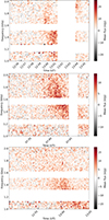 |
Fig. 4. Zoomed-in version of the dynamic spectra for the three bursts with a clear drift in time and frequency. Left: Third burst in January observation (21 January, 2018, at 13:01 UT). Middle: First burst in February observation (20 February, 2018, at 07:40 UT). Right: Second burst in February observation (20 February, 2018, at 13:00 UT). The dynamic spectra here have been constructed using an integration time of 10 seconds and frequency binning of 16 MHz. |
Properties of the five bursts that have a peak flux at least 4 times the quiescent emission levels of ∼0.5 mJy in Stokes V.
Assessing possible frequency drifts in the more structured bursts is more challenging. A closer look at the brightest burst (the first in the January observation) hints for instance at the presence of a positive frequency drift at the third substructure, but the presence of overlapping components with possibly different drifts, and the unavailability of flagged channels, prevents us from undertaking a detailed evaluation.
3.3. Information from other archival radio datasets
In addition to the band L observations that are the focus of this study, we also present here the other available information on DG CVn radio emission at different wavelengths in Fig. 5, as obtained from various archival observations over the years. The data points include: (i) the V-LoTSS (Callingham et al. 2023) observations at 144 MHz, where the source was detected with a ∼100% left circularly polarized emission of 0.5 ± 0.1 mJy; (ii) the VLASS survey (S band, 2–4 GHz), with a Stokes I flux density of 2.1 ± 0.1 mJy, 3.3 ± 0.1 mJy, and 3.5 ± 0.1 mJy in epochs 1.1, 2.1, and 3.1, respectively; (iii) the all-sky Rapid ASKAP Continuum Survey (Driessen et al. 2024) at 0.887 GHz (RACS-low; McConnell et al. 2020; Hale et al. 2021), 1.367 GHz (RACS-mid; Duchesne et al. 2023), and 1.655 GHz (RACS-high; Duchesne et al. 2025), with flux density in Stokes I ranging between ∼3–5 mJy in three pointings, while it reaches ∼10 mJy during one of the two pointings of the RACS-low survey. We have also included the Stokes V fluxes, wherever the S/N > 4. This gives the circular polarization fraction varying between 25–80% for these pointings at respective ASKAP bands.
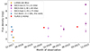 |
Fig. 5. Available radio detections of DG CVn, including the VLA band L 2018 observations analyzed in this work, and the archival data from LOFAR, ASKAP, and VLA S-band surveys, collected in the Radio Stars catalog, radiostars.org (Driessen et al. 2024). Colors identify different surveys and/or observations, with circles representing Stokes I and stars representing Stokes V detections (if available), respectively. |
Note also that the apparent long-term variability of the values is likely contaminated by the presence of bursts. The clear example is from the data of this work, for which the time-integrated flux for January and February is mostly due to the different peak values of the main bursts, rather than a different quiescent emission (which looks similar in both observations: ∼3 and ∼0.5 mJy in Stokes I and V, respectively, see Fig. 2).
4. Discussion
The analysis of these two long observations of DG CVn shows that there is an apparently quiescent, weakly polarized component, which could be ascribable to incoherent gyrosynchrotron emission coming from the magnetosphere surrounding one or both stars, even though the observed radio luminosity is orders of magnitude brighter than that predicted by Güdel-Benz relation, similar to what has also been observed for UV Cet (Bastian et al. 2022). More importantly, we have detected multiple radio bursts, ranging from short-duration bursts lasting for ≲10 minutes to ones that evolve for ≳30 minutes As can be seen in Fig. 2, all bursts are possibly fully RCP (no LL excess is seen).
In Table 2, we summarize the characteristics of the bursts, indicating the range of primary and secondary phases encompassed, frequency, drift rate, and a tentative match to the phenomenological classification of M dwarf bursts proposed by Bloot et al. (2024). We also report the luminosity, L = 4πd2FνfbΔν, where we adopt Δν = 1 GHz (the observed bandwidth) and assume a beaming fraction of fb = 1.6 sr, representative of the values for Jupiter’s auroral oval (e.g., Grießmeier et al. 2007). Additionally, we estimate the maximum size of the emitting region as Rmax = cτvar, where the variability timescale, τvar, is measured from the flux rise time of each burst. These emitting radii are upper limits, and can be tens to hundreds of times larger than the stellar radius, R⋆ = 0.72 R⊙ (Bouma et al. 2024). Such values of peak fluxes and Rmax imply lower limits on the brightness temperature, Tb ≳ 106 − 108 K. However, these limits are not constraining enough to formally provide a conclusion on the emission mechanism, but, combined with the high circular polarization, they clearly points toward coherent plasma or ECM emission. As is explained in detail by Villadsen & Hallinan (2019), it is not trivial to practically distinguish these mechanisms for a given burst in M dwarfs. In the Solar System paradigm, plasma emission is typically associated with stochastic solar flares and associated coronal mass ejections (CMEs), while ECM is often associated with auroras such as on Jupiter and possibly on the Sun (Yu et al. 2024). In M dwarfs, despite the high flaring rates in many cases, a definitive confirmation of CMEs (i.e., a huge amount of material moving outward at very high speed) is still pending (Crosley & Osten 2018; Zic et al. 2020; Mohan et al. 2024), and the much higher large-scale magnetic fields may indeed prevent them (Alvarado-Gómez et al. 2018; Villadsen & Hallinan 2019).
Considering these caveats, there are two main ways to distinguish the two mechanisms. The first one is to infer the velocity associated to the frequency drift rate. Both ECM and plasma emission can show drift in frequency over time, which could be caused by beaming effects or the motion of the source. If Hν is the scale height for the peak emission frequency, ν (where Hν is defined as the plasma density scale height for plasma emission, or the magnetic field lengthscale for ECM), the velocity of the moving source (V) can be calculated as (Villadsen & Hallinan 2019)
 (1)
(1)
Taking the negative drift rates of Table 2, and assuming Hν ∼ 0.1–1 R⋆ (which covers reasonable values, see Villadsen & Hallinan 2019), we infer a range of velocities, V ∼ 30–600 km/s. This range of values is compatible with expanding coronal loops and is much lower than the ones expected from the forward shock of a CME, which must travel at super-Alfvénic speeds and can reach up to several thousands of kilometers per second in the case of magnetized (B ∼ kG) M dwarfs (Villadsen & Hallinan 2019). However, the drift could also be due to a beaming effect, which is well documented and modeled for ECM (Hess et al. 2008) and for which we see emission coming from regions with different magnetic field strengths and/or plasma densities, as the star rotates.
The second method of inferring the underlying mechanism is observing a rotational modulation, which would favor ECM, since it would be related to specific magnetic field lines that cross the line of sight once or twice per period. This would again indicate the presence of the angular beaming characteristic of ECM as this kind of emission is primarily beamed perpendicular to the local magnetic field lines, forming a hollow-cone pattern around them and can only be detected when this beam aligns with our view. As a matter of fact, bursts in AU Mic and other M dwarfs (Bloot et al. 2024) tend to be clustered in two sections of the stellar rotational phase. In our data, the short-duration bursts (≲10 minutes long with a similar frequency drift pattern, i.e., the third burst in the January observation and second and fourth bursts in the February observation) occur around a (secondary) phase range of Φ2 ∼ 0.9–0.2, while no clear clustering is seen when the light curves are folded using the primary period. In particular, we notice the similarity in shape between the main complex bursts in January and February, happening at around Φ2 ∼ 0.8–0.15. If the phase bunching is confirmed, this might trace the magnetic field and plasma density characteristics of the emitting region, associated with the detectable beamed emission directed toward our line of sight at that phase range.
Note that we see clustering of RCP bursts only whereas AU Mic has both the LCP and RCP counterparts, but this could be a geometrical effect, which allows the observer to intersect one or both magnetic poles, and which has been invoked to explain UV Cet’s RCP-only bursts based on its magnetic map (Bastian et al. 2022). The bottom line is that, given the scarcity of data, we cannot put statistically meaningful constraints on the geometry as was done for AU Mic by Bloot et al. (2024). However, we can argue that, assuming that ECM is the mechanism underlying the coherent, polarized bursts, the local magnetic field in the emitting regions is of the same polarity, and on the order of ∼3–5 kG, although this is biased by the data availability limited to the L-band only.
We also compared the bursts observed on DG CVn with the different phenomenological classes of bursts seen on AU Mic (Bloot et al. 2024). Our observed DG CVn bursts can be tentatively assigned to type D (high drift rates, 30–60 min), F (irregular), and G (broadband, short timescales); see Table 2. Note that such a case-by-case manual classification is just meant to draw possible analogies with other M dwarfs, but can present ambiguities and has no strong physical implications. While different frequencies or temporal resolutions make detailed comparisons difficult, some similarities suggest that DG CVn shares properties with other radio-bursting M dwarfs (Zhang et al. 2023; Bloot et al. 2024; Pineda & Villadsen 2023; Bastian et al. 2022). For example, the tentative presence of G-type bursts places DG CVn in closer similarity to UV Cet, whereas no such bursts have been observed in AU Mic. This indicates that DG CVn emission properties may resemble the ones of UV Cet.
Additionally, the known binarity and SSS behavior of this source provide an interesting context, into which the radio emission can offer additional insights. In this regard, we remark the striking similarity of the radio light curves and optical photometric periodicity between DG CVn and J0508-21 (Kaur et al. 2024), which are the only two SSSs studied in detail in radio so far. In both these systems, the RR excess is seen at a specific phase (Kaur et al. 2024). The periods of SSSs are stable over a timescale of a few years at least. However, the morphology of the light curve changes. The depths of the dips and the phases at which the dips occur are stable over ∼ tens to hundreds of cycles, but rarely thousands of cycles. Figure 6 of Bouma et al. (2024) shows that none of ∼30 SSSs analyzed in their paper with a > 2-year baseline maintain a similar light curve morphology, although they usually remain complex. Because of this, and due to the loss of phase coherence over the ≳2 yr gap between the closest TESS and VLA observations, we cannot phase-connect the optical and radio light curves of DG CVn, as Kaur et al. (2024) did for J0508-21, thanks to a much smaller time gap (few months). This implies that we do not have the information needed to investigate possible correlations in phase between the radio bursts and the optical dips.
Nevertheless, if future observations confirm the bursts to be periodic on P2, it would mean that the observed radio behavior is reflecting the radio loudness of the fast rotator in the binary, and is not related to the SSS behavior, which is seen only with a periodicity, P1. This would suggest that the coherent bursts are more directly linked to stellar youth and rapid rotation, as in the case of AU Mic, rather than being caused by transiting material at the corotation radius. We highlight the need for simultaneous optical and radio observations to have multiple cycles close in time, with minimum evolution of the obscuring material. Ultimately, simultaneous multiwavelength monitoring will be key to uncovering the true driver of the coherent bursts, whether rooted in stellar magnetism, rotation, or circumstellar dynamics.
Acknowledgments
SK carried out this work within the framework of the doctoral program in Physics of the Universitat Autònoma de Barcelona. SK, OM, and DV are supported by the European Research Council (ERC) under the European Union’s Horizon 2020 research and innovation programme (ERC Starting Grant “IMAGINE” No. 948582). E.I. acknowledges funding from the European Research Council under the European Union’s Horizon Europe programme (grant number 101042416 STORMCHASER). We acknowledge financial support from the Agencia Estatal de Investigación (AEI/10.13039/501100011033) of the Ministerio de Ciencia e Innovación and the ERDF “A way of making Europe” through projects PID2023-146675NB-100, PID2022-137241NB-C4[1:4], PID2021-125627OB-C31, PID2020-117710GB-100, PID2020-117404GB-C21, PID2023-147883NB-C21, and the Centre of Excellence “Severo Ochoa”/“María de Maeztu” awards to the Institut de Ciències de l’Espai (CEX2020-001058-M), Instituto de Astrofísica de Canarias (CEX2019-000920-S), and Instituto de Astrofísica de Andalucía (CEX2021-001131-S). The National Radio Astronomy Observatory and Green Bank Observatory are facilities of the U.S. National Science Foundation operated under cooperative agreement by Associated Universities, Inc.
References
- Alissandrakis, C. E. 1986, Sol. Phys., 104, 207 [CrossRef] [Google Scholar]
- Alvarado-Gómez, J. D., Drake, J. J., Cohen, O., Moschou, S. P., & Garraffo, C. 2018, ApJ, 862, 93 [Google Scholar]
- Bastian, T. S., Cotton, W. D., & Hallinan, G. 2022, ApJ, 935, 99 [NASA ADS] [CrossRef] [Google Scholar]
- Bell, C. P. M., Mamajek, E. E., & Naylor, T. 2015, MNRAS, 454, 593 [Google Scholar]
- Beuzit, J. L., Ségransan, D., Forveille, T., et al. 2004, A&A, 425, 997 [NASA ADS] [CrossRef] [EDP Sciences] [Google Scholar]
- Bloot, S., Callingham, J. R., Vedantham, H. K., et al. 2024, A&A, 682, A170 [NASA ADS] [CrossRef] [EDP Sciences] [Google Scholar]
- Bouma, L. G., Jayaraman, R., Rappaport, S., et al. 2024, AJ, 167, 38 [NASA ADS] [CrossRef] [Google Scholar]
- Callingham, J. R., Shimwell, T. W., Vedantham, H. K., et al. 2023, A&A, 670, A124 [NASA ADS] [CrossRef] [EDP Sciences] [Google Scholar]
- CASA Team (Bean, B., et al.) 2022, PASP, 134, 114501 [NASA ADS] [CrossRef] [Google Scholar]
- Chabrier, G. 2001, ApJ, 554, 1274 [NASA ADS] [CrossRef] [Google Scholar]
- Comrie, A., Wang, K. S., Hsu, S. C., et al. 2021, https://doi.org/10.5281/zenodo.4905459 [Google Scholar]
- Cortés-Contreras, M., Béjar, V. J. S., Caballero, J. A., et al. 2017, A&A, 597, A47 [NASA ADS] [CrossRef] [EDP Sciences] [Google Scholar]
- Crosley, M. K., & Osten, R. A. 2018, ApJ, 862, 113 [NASA ADS] [CrossRef] [Google Scholar]
- Driessen, L. N., Pritchard, J., Murphy, T., et al. 2024, PASA, 41, e084 [NASA ADS] [CrossRef] [Google Scholar]
- Duchesne, S. W., Thomson, A. J. M., Pritchard, J., et al. 2023, PASA, 40 [Google Scholar]
- Duchesne, S. W., Ross, K., Thomson, A. J. M., et al. 2025, PASA, 42, e038 [Google Scholar]
- Dulk, G. A. 1985, ARA&A, 23, 169 [Google Scholar]
- Engle, S. G., & Guinan, E. F. 2023, ApJ, 954, L50 [NASA ADS] [CrossRef] [Google Scholar]
- Farrell, W. M., Desch, M. D., & Zarka, P. 1999, J. Geophys. Res., 104, 14025 [NASA ADS] [CrossRef] [Google Scholar]
- Fender, R. P., Anderson, G. E., Osten, R., et al. 2015, MNRAS, 446, L66 [Google Scholar]
- Gaia Collaboration (Brown, A. G. A., et al.) 2021, A&A, 649, A1 [NASA ADS] [CrossRef] [EDP Sciences] [Google Scholar]
- Grießmeier, J. M., Zarka, P., & Spreeuw, H. 2007, A&A, 475, 359 [NASA ADS] [CrossRef] [EDP Sciences] [Google Scholar]
- Günther, M. N., Zhan, Z., Seager, S., et al. 2020, AJ, 159, 60 [Google Scholar]
- Hale, C. L., McConnell, D., Thomson, A. J. M., et al. 2021, PASA, 38, e058 [NASA ADS] [CrossRef] [Google Scholar]
- Helfand, D. J., Schnee, S., Becker, R. H., White, R. L., & McMahon, R. G. 1999, AJ, 117, 1568 [Google Scholar]
- Henry, T. J., Jao, W.-C., Subasavage, J. P., et al. 2006, AJ, 132, 2360 [Google Scholar]
- Hess, S., Cecconi, B., & Zarka, P. 2008, Geophys. Res. Lett., 35, L13107 [NASA ADS] [CrossRef] [Google Scholar]
- Joseph, W. M., Stelzer, B., Magaudda, E., & Vičánek Martínez, T. 2024, A&A, 688, A49 [NASA ADS] [CrossRef] [EDP Sciences] [Google Scholar]
- Kaur, S., Viganò, D., Béjar, V. J. S., et al. 2024, A&A, 691, L17 [NASA ADS] [CrossRef] [EDP Sciences] [Google Scholar]
- Kavanagh, R. D., Vedantham, H. K., Rose, K., & Bloot, S. 2024, A&A, 692, A66 [NASA ADS] [CrossRef] [EDP Sciences] [Google Scholar]
- Koen, C. 2021, MNRAS, 500, 1366 [Google Scholar]
- McConnell, D., Hale, C. L., Lenc, E., et al. 2020, PASA, 37, e048 [Google Scholar]
- McLean, M., Berger, E., Irwin, J., Forbrich, J., & Reiners, A. 2011, ApJ, 741, 27 [NASA ADS] [CrossRef] [Google Scholar]
- Melrose, D. B. 2017, Rev. Mod. Plasma Phys., 1, 5 [Google Scholar]
- Melrose, D. B., & Dulk, G. A. 1982, ApJ, 259, 844 [Google Scholar]
- Mohan, A., Gopalswamy, N., Mondal, S., Kumari, A., & Gunaseelan, S. 2024, AGU Fall Meeting Abstracts, 2024, SH53A-295 [Google Scholar]
- Osten, R. A., Kowalski, A., Drake, S. A., et al. 2016, ApJ, 832, 174 [Google Scholar]
- Ott, J., Raba, R., & Hibbard, J. 2022, Am. Astron. Soc. Meeting Abstr., 54, 215.05 [Google Scholar]
- Pineda, J. S., & Villadsen, J. 2023, Nat. Astron., 7, 569 [NASA ADS] [CrossRef] [Google Scholar]
- Reiners, A., Shulyak, D., Käpylä, P. J., et al. 2022, A&A, 662, A41 [NASA ADS] [CrossRef] [EDP Sciences] [Google Scholar]
- Riedel, A. R., Finch, C. T., Henry, T. J., et al. 2014, AJ, 147, 85 [NASA ADS] [CrossRef] [Google Scholar]
- Smith, K., Pestalozzi, M., Güdel, M., Conway, J., & Benz, A. O. 2003, A&A, 406, 957 [NASA ADS] [CrossRef] [EDP Sciences] [Google Scholar]
- Stauffer, J., Collier Cameron, A., Jardine, M., et al. 2017, AJ, 153, 152 [Google Scholar]
- Villadsen, J., & Hallinan, G. 2019, ApJ, 871, 214 [Google Scholar]
- Waugh, R. F. P., & Jardine, M. M. 2022, MNRAS, 514, 5465 [CrossRef] [Google Scholar]
- Yiu, T. W. H., Vedantham, H. K., Callingham, J. R., & Günther, M. N. 2024, A&A, 684, A3 [NASA ADS] [CrossRef] [EDP Sciences] [Google Scholar]
- Yu, S., Chen, B., Sharma, R., et al. 2024, Nat. Astron., 8, 50 [Google Scholar]
- Zarka, P. 2004, Adv. Space Res., 33, 2045 [NASA ADS] [CrossRef] [Google Scholar]
- Zhan, Z., Günther, M. N., Rappaport, S., et al. 2019, ApJ, 876, 127 [Google Scholar]
- Zhang, J., Tian, H., Zarka, P., et al. 2023, ApJ, 953, 65 [NASA ADS] [CrossRef] [Google Scholar]
- Zic, A., Stewart, A., Lenc, E., et al. 2019, MNRAS, 488, 559 [Google Scholar]
- Zic, A., Murphy, T., Lynch, C., et al. 2020, ApJ, 905, 23 [Google Scholar]
Appendix A: TESS light curves
We present the phase-folded 2-minutes cadence TESS light curves of DG CVn, aka TIC 368129164, in Fig. A.1. Compared to Bouma et al. (2024) where sectors 23 (March-April 2020, left column) and 50 (March-April 2022, middle column) have been reported, here we add a third available TESS sector 77 (March-April 2024), and, besides folding the light curves with P1 (top panels), we focus also on the modulation with the second period, P2 (second row panels). The third row shows the folding with P1 after removing the P2 signal, which clearly decreases the dispersion of the points at a given phase.
If we interpret the periods as the rotational spins of the two stars, this implies that the SSS behavior is associated to the slowest of the two components only. Moreover, as in many other SSSs, within a given sector the light curve show consistently repeating features (and frequent, stochastic flares), but from one sector to another the dips shift in phase and shape. Indeed, dips are almost invisible in sector 23, only tentatively seen around ϕ1 = 0.25 (indeed dubbed as ambiguous by Bouma et al. 2024). The change in shape is likely indicative of the variability of the optical depth and/or size of the obscuring material. The shift in phase could be one or more of the following reasons: (i) intrinsic, due a non-perfectly corotating orbit or, equivalently, a shift in the phase position of the obscuring material or the magnetic field lines that trap the material; (ii) indicative of the lifetime of opaque clumps (related to disk debris and/or disintegrating planet), forming and fading away at different phases over the years; (iii) importantly, caused by the loss of phase coherence after typically  (yr), due to the uncertainty on the dip phase, which eq. (9) in Bouma et al. (2024) evaluated as δϕ ∼ 0.02 Δt/(20 d) after a period Δt (specifically, δϕ ∼ 0.8, i.e. a complete loss of phase coherence, considering the Δt ∼ 2.2 yr between the latest VLA and the earliest TESS observations).
With TESS data only, we cannot favor any of the three explanations above, and more discussion about this issues, common in SSSs, can be found in Bouma et al. (2024). In this sense, more details of a dedicated, on-going, multi-instrument photometric campaign will be the object of a dedicated study, while this article is focused on the radio emission alone.
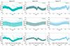 |
Fig. A.1. Simple Aperture Photometry flux light curves of TESS sectors 23 (left column), 50 (middle column) and 77 (right column), with a cadence of 2 minutes. The top row represents the normalized flux phase folded with the primary period of P1 = 6.44 hours while the middle row represents the same normalized flux phase folded with the secondary period of P2 = 2.60 hours. In the third row, we present the flux folded with the primary period, but after removing the secondary signal. In all these light curves, the phase is arbitrarily set by fixing Φ = 0 at the beginning of the first target scan of VLA January observation (21/01/2018-07:17:00 UT), as in the rest of the paper. |
All Tables
Properties of the five bursts that have a peak flux at least 4 times the quiescent emission levels of ∼0.5 mJy in Stokes V.
All Figures
|
Fig. 1. Combined map for the January and February observations, centered at the emission peak, which shows an offset from the SIMBAD position that is compatible with the reported proper motion of DG CVn. The synthesized beam is shown in the lower left corner and the cross (+) marks the proper motion corrected position. The color scale represents the Stokes I flux density, while the contours indicate the Stokes V signal, corresponding to levels of 5, 10, 20, 30, 40, and 50 σrmsV (where σrmsV is ∼11.2 μJy/beam). |
| In the text | |
|
Fig. 2. Phase-aligned light curves for LL and RR correlations using the primary period P1 = 6.44 h (top) and the secondary period P2 = 2.60 h (bottom), reported in Bouma et al. (2024). The flux represents the peak flux values on a logarithmic scale extracted from the image planes of each 5-minute scan, using the CASA task imfit. Here, phase |
| In the text | |
|
Fig. 3. Dynamic spectra for Stokes V for January (top) and February (bottom) observations, taken from visibility plane. The error bars in the light curves and frequency spectrum represent the standard deviation, computed by considering the imaginary component of the amplitude. The top and bottom axes of the top panel represent the primary and secondary phases (Φ1 and Φ2), respectively, calculated using the primary and secondary periods reported in Bouma et al. (2024). We fixed the reference phase Φ = 0 at the beginning of the first target scan in the January observation. The vertical blue lines indicate the start (Φ = 0) of new primary (dashed) and secondary (solid) cycles, respectively. |
| In the text | |
|
Fig. 4. Zoomed-in version of the dynamic spectra for the three bursts with a clear drift in time and frequency. Left: Third burst in January observation (21 January, 2018, at 13:01 UT). Middle: First burst in February observation (20 February, 2018, at 07:40 UT). Right: Second burst in February observation (20 February, 2018, at 13:00 UT). The dynamic spectra here have been constructed using an integration time of 10 seconds and frequency binning of 16 MHz. |
| In the text | |
|
Fig. 5. Available radio detections of DG CVn, including the VLA band L 2018 observations analyzed in this work, and the archival data from LOFAR, ASKAP, and VLA S-band surveys, collected in the Radio Stars catalog, radiostars.org (Driessen et al. 2024). Colors identify different surveys and/or observations, with circles representing Stokes I and stars representing Stokes V detections (if available), respectively. |
| In the text | |
|
Fig. A.1. Simple Aperture Photometry flux light curves of TESS sectors 23 (left column), 50 (middle column) and 77 (right column), with a cadence of 2 minutes. The top row represents the normalized flux phase folded with the primary period of P1 = 6.44 hours while the middle row represents the same normalized flux phase folded with the secondary period of P2 = 2.60 hours. In the third row, we present the flux folded with the primary period, but after removing the secondary signal. In all these light curves, the phase is arbitrarily set by fixing Φ = 0 at the beginning of the first target scan of VLA January observation (21/01/2018-07:17:00 UT), as in the rest of the paper. |
| In the text | |
Current usage metrics show cumulative count of Article Views (full-text article views including HTML views, PDF and ePub downloads, according to the available data) and Abstracts Views on Vision4Press platform.
Data correspond to usage on the plateform after 2015. The current usage metrics is available 48-96 hours after online publication and is updated daily on week days.
Initial download of the metrics may take a while.