| Issue |
A&A
Volume 701, September 2025
|
|
|---|---|---|
| Article Number | A3 | |
| Number of page(s) | 11 | |
| Section | Astronomical instrumentation | |
| DOI | https://doi.org/10.1051/0004-6361/202555228 | |
| Published online | 28 August 2025 | |
Cross-calibration of the energy response of the gamma-ray detectors on board GECAM-B
1
State Key Laboratory of Particle Astrophysics, Institute of High Energy Physics, Chinese Academy of Sciences,
Beijing
100049,
China
2
University of Chinese Academy of Sciences,
Beijing
100049,
China
3
College of Physics and Hebei Key Laboratory of Photophysics Research and Application, Hebei Normal University,
Shijiazhuang, Hebei
050024,
China
4
Shijiazhuang Key Laboratory of Astronomy and Space Science, Hebei Normal University, Shijiazhuang,
Hebei
050024,
China
5
Guizhou Provincial Key Laboratory of Radio Astronomy and Data Processing, Guizhou Normal University,
Guiyang
550001,
PR China
6
School of Physics and Electronic Science, Guizhou Normal University,
Guiyang
550001,
PR China
7
School of Computer and Information, Dezhou University,
Dezhou
253023,
Shandong,
China
8
School of Physics and Optoelectronics, Xiangtan University,
Xiangtan
411105,
Hunan,
China
9
Institute of Astrophysics, Central China Normal University,
Wuhan
430079,
China
★ Corresponding authors: This email address is being protected from spambots. You need JavaScript enabled to view it.
; This email address is being protected from spambots. You need JavaScript enabled to view it.
; This email address is being protected from spambots. You need JavaScript enabled to view it.
Received:
21
April
2025
Accepted:
26
June
2025
Abstract
Context. The Gravitational-wave high-energy Electromagnetic Counterpart All-sky Monitor (GECAM) was primarily designed to detect gamma-ray bursts (GRBs), particularly those associated with gravitational-wave events. The energy response of detectors plays a crucial role in detection performance and scientific data analysis.
Aims. We applied the cross-calibration methodology to calibrate and optimize the energy response of the gamma-ray detectors (GRDs) on board GECAM-B, using eight GRBs that were jointly observed by GECAM-B and other well-calibrated instruments. These GRBs enable the comprehensive calibration of all GRDs with different incident angles.
Methods. Cross-calibration using well-calibrated instruments is the most efficient way to verify the energy response of the detectors. The basic approach involves performing a joint spectral analysis and introducing a constant factor to quantify the difference in effective area between instruments. This calibration method has been widely used in the cross-calibration of many high-energy astrophysical instruments.
Results. We completed the cross-calibration of all 25 GRDs, covering two electronics readout channels and different incidence angles. The results of the joint spectral fitting demonstrate that GECAM-B exhibits good consistency with the well-calibrated Fermi/GBM instrument. Furthermore, the GECAM-B energy response matrix accurately reproduces the observational data without requiring any corrections or modifications.
Conclusions. Thanks to the broad energy band, accurate energy response, and anti-saturation design, GECAM-B can constrain spectral models and measure spectral parameters for not only typical bursts but also exceptionally bright events, including GRB 221009A and GRB 230307A, the two brightest GRBs ever detected.
Key words: instrumentation: detectors / methods: data analysis / telescopes
© The Authors 2025
 Open Access article, published by EDP Sciences, under the terms of the Creative Commons Attribution License (https://creativecommons.org/licenses/by/4.0), which permits unrestricted use, distribution, and reproduction in any medium, provided the original work is properly cited.
This article is published in open access under the Subscribe to Open model. This email address is being protected from spambots. You need JavaScript enabled to view it. to support open access publication.
1 Introduction
The Gravitational-wave high-energy Electromagnetic Counterpart All-sky Monitor (GECAM) is designed for the detection of high-energy gamma-ray transients, including the gammaray electromagnetic counterparts of gravitational waves and fast radio bursts (Wang et al. 2022), gamma-ray bursts (GRBs; An et al. 2023; Zhang et al. 2024; Zheng et al. 2024a), soft gammaray repeaters (Xiao et al. 2024a,b,c; Xie et al. 2025), and solar flares (Zhao et al. 2023a), as well as terrestrial gamma-ray flashes and terrestrial electron beams (Zhao et al. 2023b). As of 2024, GECAM had evolved into a constellation consisting of two micro-satellites and two payloads carried on experimental satellites.
The first two micro-satellites, GECAM-A and GECAM-B (Li et al. 2022), were launched on December 10, 2020 (UTC+8). Due to the power supply issues of the satellite platform, the observational capabilities of both GECAM-A and GECAM-B are partially constrained. To enhance the overall performance of the GECAM mission, GECAM-C (also known as the High Energy Burst Searcher; Zhang et al. 2023a; Zheng et al. 2024b; Zhang et al. 2023b) on board the SATech-01 experimental satellite and GECAM-D (also known as the Gamma-ray Transient Monitor; Feng et al. 2024) on board the DRO-A satellite were launched in July 2022 and March 2024, respectively.
With capabilities such as real-time triggering, localizing bursts in orbit (Zhao et al. 2024), high-precision timing (Xiao et al. 2022a), near-real-time data download via the BeiDou navigation satellite (Chen et al. 2020; Huang et al. 2024), and accurate ground-based localization (Xiao et al. 2021, 2022b; Zhao et al. 2023c), GECAM represents a significant high-energy telescope in the era of multi-messenger astronomy. Notably, GECAM has made remarkable contributions to the observation of peculiar burst events, including the brightest ever GRBs ever detected, GRB 221009A (An et al. 2023; Zhang et al. 2024; Zheng et al. 2024a) and GRB 230307A (Yi et al. 2025; Sun et al. 2025), as well as the second X-ray burst associated with a fast radio burst (Wang et al. 2022).
Compared to classic photomultiplier, the silicon photomultiplier (SiPM) offers several advantages, including high quantum efficiency, high gain (105 ∼ 106), low operating voltage, insensitivity to magnetic fields, and ease of integration. Consequently, GECAM-A and GECAM-B are each equipped with 25 SiPM-based gamma-ray detectors (GRDs; An et al. 2022) and 8 SiPM-based charged particle detectors (CPDs; Xu et al. 2022). The GRDs are designed to detect gamma-ray photons, while the CPDs help monitor the space particle environment; charged particle events can be identified by comparing the count rate ratio between the CPDs and the GRDs. Despite the power supply limitations, GECAM-B has consistently detected numerous astrophysical high-energy transient sources, whereas GECAM-A has not been able to observe regularly.
Instrument calibration serves as the foundation for performance validation, scientific observations, and data analysis. Ground-based experimental calibration and simulation analyses have been carried out to evaluate the performance of GECAM-B (He et al. 2023; Guo et al. 2020; Zhang et al. 2019), thereby contributing to the construction of its energy response matrix. In-flight energy calibration of the GRDs, including the energychannel and energy-resolution relationships, was also conducted using characteristic gamma-ray lines present in the background spectra (Qiao et al. 2024).
In this study, we primarily validated the energy response of GECAM-B through the cross-calibration method with other well-calibrated instruments and determined the optimal energy ranges for spectral analysis across both the high-gain and low-gain readout channels of each detector. This paper is structured as follows: A detailed introduction of GECAM-B as well as the Fermi Gamma-ray Burst Monitor (GBM) is given in Sect. 2. Data reduction and our analysis method are presented in Sect. 3. Cross-calibration results are provided and discussed in Sects. 4 and 5, respectively. Finally, a summary is given in Sect. 6.
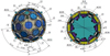 |
Fig. 1 Schematic diagram of the installation position of the GRDs in GECAM. |
2 Calibration instruments
2.1 GECAM-B
GECAM-A and GECAM-B are two micro-satellites of the GECAM constellation. Each micro-satellite is equipped with 25 round-shaped GRDs and 8 square-shaped CPDs, oriented in various directions to cover a very large field of view, as illustrated in Fig. 1.
The GRDs utilize LaBr3 scintillators coupled with SiPM arrays to detect gamma-ray photons. A pre-amplifier placed behind the SiPM arrays is used to shape the output signals and direct them into two readout channels: high-gain and low-gain channels. This dual-channel configuration enables the energy spectrum measurement of high-energy transient sources in the range of 6 keV to 5 MeV, which has been verified by on-ground calibration (Lv et al. 2018; Zhang et al. 2022a; He et al. 2023; Zheng et al. 2022).
Prior to the launch of both GECAM-A and GECAM-B, extensive ground calibration experiments were conducted using the Hard X-ray Calibration Facility (He et al. 2023) and radioactive sources (An et al. 2022; Li et al. 2022), covering the majority of the energy range for which GECAM-A and GECAM-B are designed. By employing incident photons of known energy, we established the precise relationship between photon energy and electronic channel values (i.e., the E-C relationship), and calibrated the energy resolution relationship and intrinsic detection efficiency. The experimental results exhibit good agreement with the simulation results (He et al. 2023).
Since the launch of GECAM, GECAM-A has been unable to perform regular observations due to power supply issues with the satellite platform. Consequently, this study focuses on GECAM-B. A detailed in-orbit energy calibration (i.e., energy-channel and resolution) of the GRD was conducted using characteristic gamma-ray lines identified in the background spectra, and it will be updated periodically (Qiao et al. 2024).
As a semiconductor device, SiPM is sensitive to temperature variation and susceptible to irradiation damage, both of which can lead to gain drift. Ground-based experiments established a correlation between temperature and SiPM bias voltage to address temperature sensitivity. Accordingly, a temperature sensor installed on the SiPM circuit board continuously monitors the local environmental temperature, enabling real-time adjustment of the SiPM bias voltage to stabilize the gain. This temperature compensation mechanism was implemented on GECAM to help maintain gain stability to within a 2% variation in orbit (Zhang et al. 2022a,b).
Due to the accumulated irradiation damage during the inorbit operation, the gain of the SiPMs has gradually decreased by up to 5% per month, while the dark current has steadily increased, resulting in a progressive rise in electronic noise over time (Qiao et al. 2024). Consequently, the effective energy range for spectral fitting has shifted to approximately 20 keV–5 MeV as of 2022 (refer to Table A.2 for specific values).
The energy response matrix of GRDs is generated through comprehensive simulations using GEANT4 (Guo et al. 2020). Importantly, the simulations account for both the direct interactions between incident photons and the detector materials, as well as the contributions from atmospheric scattering. However, since electronic processes and other factors could not been fully modeled within GEANT4 for GECAM, the results must be further corrected using both ground-based and in-orbit calibration data to produce an accurate detector energy response matrix.
Information about the GRBs used for cross-calibration.
2.2 Fermi/GBM
The GBM, as one of two instruments on board the Fermi Gamma-Ray Space Telescope, comprises 12 NaI (Sodium Iodide) detectors sensitive to energies from 8 keV to 1 MeV, and 2 BGO (Bismuth Germanate) detectors covering the 200 keV to 40 MeV range (Meegan et al. 2009). With its broad energy coverage encompassing the entire detection range of GECAM-B, and its calibration cross-validated with other instruments since launch (Tierney et al. 2011; Stamatikos 2009; Von Kienlin et al. 2009), Fermi/GBM serves as an ideal instrument for cross-calibration of GECAM-B.
For joint spectral analysis, we selected the two NaI detectors with the highest count rates, along with the BGO detector located on the same side as the selected NaI detector1. The installation configuration of Fermi/GBM detectors can be found in Bissaldi et al. (2009). Three types of scientific data products from Fermi/GBM are available for download from the Fermi data archive2 and were preprocessed using GBM Data Tools package (Goldstein et al. 2022).
3 Data reduction and analysis method
Before performing cross-calibration, appropriate calibration samples should be selected, as outlined in Sect. 3.1. Subsequently, the basic energy spectrum model for the calibration and the calibration method are introduced in Sects. 3.2 and 3.3, respectively.
3.1 GRB samples
We selected GRBs observed simultaneously by GECAM-B and the Fermi/GBM. These samples were selected based on the following criteria: (a) joint observations, (b) sufficient brightness, and (c) relatively accurate location. The list of GRBs selected based on these criteria is presented in Table 1, which contains key information such as the burst number, trigger time, selected time intervals for cross-calibration, and GRB localization. In addition, the calibrated GECAM-B detectors and their corresponding incident angles for each GRB are listed in Table A.1.
3.2 Spectral model
The band (Band et al. 1993) and cutoff power-law (Von Kienlin et al. 2014) models are adopted for the joint spectral fitting. Both models are commonly used in GRB spectral analysis, and their mathematical forms are briefly described as follows:
![Mathematical equation: \rm N_{Band}(E)=\left\{ \begin{aligned} &\rm A \bigg (\frac{\rm E}{100 \enspace \rm keV}\bigg )^{\rm \alpha} exp\bigg(-\frac{\rm E}{\rm E_{cut}}\bigg ), (\rm \alpha -\beta)\rm E_{cut} \geq \rm E, \\ &\rm A \bigg [\frac{(\rm \alpha-\rm \beta) \rm E_{cut}} {100\enspace \rm keV}\bigg ]^{\rm \alpha-\rm \beta} exp(\rm \beta-\rm \alpha)\bigg (\frac{\rm E}{100\enspace \rm keV}\bigg )^{\rm \beta}, (\rm \alpha -\rm \beta) \rm E_{cut} \leq \rm E, \end{aligned} \right.](/articles/aa/full_html/2025/09/aa55228-25/aa55228-25-eq1.png)
where A is the normalization amplitude constant (in units of photons · cm−2 · s−1 · keV−1) at 1 keV, α and β are the power law low-energy and high-energy spectral indices, which are separated by the characteristic cutoff energy Ecut in keV:
 (1)
(1)
where A is the normalization amplitude constant (photons · cm−2 · s−1 · keV−1), α is the power-law photon index, and Ecut is the characteristic cutoff energy in keV.
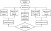 |
Fig. 2 Cross-calibration process. |
3.3 Calibration methods
As discussed in Sect. 3.2, multiple spectral models are available for cross-calibration. Individual spectral fitting is performed using well-calibrated instruments to determine the most appropriate spectrum model. To account for the measurement inconsistencies between GECAM-B and other instruments, including different GRDs and both high-gain and low-gain channels, constant factors are introduced to quantify the effective area differences among the various instruments.
Furthermore, the constant factor for the well-calibrated instrument (as the baseline) is fixed to 1. This calibration approach has been widely employed in the cross-calibration of numerous high-energy astrophysical instruments (Stamatikos 2009; Von Kienlin et al. 2009; Tierney et al. 2011; Luo et al. 2020; Sakamoto et al. 2011).
4 Cross-calibration and results
The cross-calibration procedure and corresponding analysis results are presented in Sects. 4.1 and 4.2, respectively. Preliminary results indicate that GECAM-B shows good agreement with Fermi/GBM.
4.1 Cross-calibration process
The complete procedure for the cross-calibration of GECAM-B’s energy response is outlined in Fig. 2 and consists of four key steps:
- (a)
An essential step must be completed before the joint crosscalibration can be formally conducted. The spectral model that best describes the GRB must be selected. To achieve this, spectrum fitting should be performed using data from well-calibrated instruments across various models, and the best model would be selected based on the Bayesian information criterion (BIC; Liddle 2007; Brownlee 2019).
- (b)
Since a well-calibrated instrument is used to determine the best-fit spectral model, the fitting results are regarded as the true GRB spectrum profile. The ideal net deposited count spectrum is obtained by convolving this GRB spectral model with the energy response matrix of GECAM-B. By comparing the ideal spectrum to the actual detected net count spectrum, the available energy range of GECAM-B can be determined.

Fig. 3 Schematic diagram of spectra without fitting. The black and red dots represent the high-gain and the low-gain data, respectively, while the black and red lines correspond to the ideal net deposited count spectra for the High-Gain and the Low-Gain channels.
As shown in Fig. 3, the energy range where the data points align well with the model lines defines the available energy range, indicating that the energy response matrix of GECAM-B accurately characterizes the data within this interval. Due to the influence of electrical noise, data acquisition thresholds are set at the low-energy ends of both gain channels. However, since the energy response matrix does not account for the associated reduction in detection efficiency near these thresholds, it fails to accurately reproduce the observed data in that region. Therefore, the energy range below the thresholds should be excluded from the spectral analysis.
Furthermore, the energy range near the K-shell absorption edges of LaBr3 is not ignored (Br: 13.47 keV, La: 38.93 keV). This is because comprehensive calibration experiments were conducted in these regions, which showed good agreement with the GEANT4-based simulations. These results indicate that the GRD energy response matrix can reliably reproduce spectral features near the K-shell absorption edges, thereby ensuring the accuracy of the energy response in this critical regime.
The top panel of Fig. 4 displays the deposited count spectrum of the high-gain channel, where a sharp decline is observed at both the low- and high-energy ends due to the influence of the detector’s data acquisition threshold on the detection efficiency. The K-shell absorption edge of La is visible around 38.93 keV. The bottom panel shows the low-gain channel deposited count spectrum. The characteristic peak of 183La at 1470 keV, which is utilized for in-orbit calibration, and both the α particle peak and the saturation peak are evident in the spectrum. Notably, the upper limit of the available energy range is constrained by the saturation peak in the low-gain channel (Liu et al. 2022).
- (c)
After determining the appropriate energy range, joint spectral analysis can proceed. Based on the source location of GRB and the attitude information of GECAM-B, the incidence angle (angle between the incident direction and the detector’s normal direction) θ in the coordinate system of each detector can be calculated. This allows us to identify a list of detectors with smaller viewing angles that are suitable for calibration with the given GRB source. To ensure consistency between the high-gain and low- gain channels of each detector, two fitting strategies are employed in the joint analysis: (1) the high-gain and low-gain channels are jointly fitted, and (2) the high-gain and low-gain channels are fitted independently.
- (d)
Subsequently, a multi-detector combined analysis is per- formed, as shown in Fig. 5, which presents the results of the joint spectral fitting for GRB 210606B. From the residual panel in Fig. 5, it is evident that the residuals are ran- domly distributed around zero without significant structures, indicating a good quality of the spectral fit. Furthermore, the strong consistency between GECAM-B and Fermi/GBM suggests that the energy response matrix of the GRDs on GECAM-B provides an accurate characterization of the observational data.
Similar to step (c), two cases should be analyzed, which helps in assessing both the consistency between different detectors and the overall agreement between GECAM-B and other instruments.
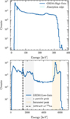 |
Fig. 4 Deposited counts spectra of the GRD01 detector in high-gain (top) and low-gain (bottom) channels. |
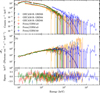 |
Fig. 5 Joint fitting result of GRB 210606B with Fermi/GBM and GECAM in the Cuttoffpl model. |
Spectral fitting results of Fermi/GBM only.
4.2 Cross-calibration results
Spectrum fittings were performed separately using Fermi/GBM alone and joint data of Fermi/GBM and GECAM-B. For the energy range selection of Fermi/GBM, two NaI(Tl) detectors were used within the 8–900 keV range, and the correspond- ing BGO detectors covered 280–35 000 keV. In addition, the 30–40 keV range was ignored for NaI(Tl) due to the Iodine K- shell absorption edge. For GECAM-B, the energy range was determined based on the criteria described in Sect. 4.1. The spectrum fitting results are presented in Tables 2 and 3. Table 2 summarizes results from the Fermi/GBM-only fitting, while Table 3 shows the joint fitting results obtained using Fermi/GBM and GECAM-B data, with three GRDs selected based on their relatively significant signals.
In Fig. 6, the fitted parameters of the spectral models are plotted. The horizontal axis represents the results from the Fermi/GBM-only fitting, while the vertical axis corresponds to the joint fitting results of Fermi/GBM and GECAM-B. The results demonstrate that the joint fitting results for GECAM-B and Fermi/GBM are highly consistent with those derived from Fermi/GBM alone.
As discussed in Sect. 4.1, joint spectrum fittings were also conducted for individual GECAM-B detectors under two scenarios. The corresponding constant factors are displayed in Figs. 7 and 8. Notably, the constant factors are close to 1, indicating strong consistency between high-gain and low-gain channels within individual GRDs, as well as between GECAM-B and Fermi/GBM. Those results demonstrate the reliability of the GECAM-B GRD energy response matrix.
Figure 9 illustrates the relationship between the calibration constant factors and the GRB flux. As the flux increases, indicating a brighter burst, the statistical uncertainties decrease, leading to tighter constraints on the constant factor. For sufficiently bright bursts, the more detailed features of the energy response can be revealed. Our results show that, although some GRDs exhibit slightly higher deviations, the overall calibration remains consistent across detectors. It is normal and acceptable, as also presented in Konus-Wind (Sakamoto et al. 2011), Swift Burst Alert Telescope (BAT) (Sakamoto et al. 2011), and Insight-Hard X-ray Modulation Telescope (Insight-HXMT) CsI detectors (Zheng et al. 2025), among others. Importantly, among the 25 GRDs on board GECAM-B, we can always select GRDs with favorable incident angles. These selections can reduce systematic uncertainties introduced by satellite structures or off-axis responses.
Joint spectral fitting results of Fermi/GBM and three GRDs of GECAM-B.
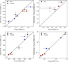 |
Fig. 6 Comparison of spectral fitting results: Fermi/GBM only vs. joint Fermi/GBM and GECAM-B. The black dashed line denotes the one-to-one correlation. Different colors indicate different spectral models, and each data point corresponds to an individual GRB. |
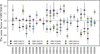 |
Fig. 7 Constant of GECAM-B detectors with the high and low gains bound together. |
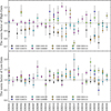 |
Fig. 8 Fitting constant of GECAM-B detectors with the high and low gains separated. |
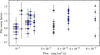 |
Fig. 9 Relationship between constant factors and GRB’s flux. |
5 Discussion
As indicated in Sect. 3.1, all 25 GRDs on board GECAM-B have been cross-calibrated, covering a wide range of incidence angles. The spectral fitting results presented in Sect. 4.2 demonstrate that GECAM-B exhibits good consistency with Fermi/GBM, suggesting that the current energy response matrix of GECAM-B can accurately describe the observation data within the defined energy range.
Notably, GECAM-B enhances the capability to constrain spectral model parameters due to two key advantages: (1) GECAM-B can help improve the statistics by having more photon counts from a burst; and (2) the 25 GRDs of GECAM-B are oriented in different directions, allowing for the selection of detectors with favorable incidence angles, thereby reducing systematic errors of observation and data analysis. If the number of detectors is limited, it will be impossible to select a detector with a good viewing angle for some bursts. This crucial role is illustrated in Fig. 6, where the vertical error (from joint fitting) is significantly smaller than the horizontal ones (from GBM-only fitting) for most GRBs. One data point for the β parameter deviates slightly from the black dashed line. This deviation arises from the limited number of photons detected by Fermi/GBM above 500 keV, resulting in a poor constraint on β. The inclusion of GECAM-B data greatly improves the constraint on the β parameter.
Additionally, we compared the actual net counts detected by Fermi/GBM and GECAM-B across the selected GRB calibration samples. Detectors with an incidence angle of less than 80 degrees were selected, as detailed in Table 4. As illustrated in Fig. 10, for most GRBs, the net counts detected by GECAM-B are comparable to or exceed those detected by Fermi/GBM. This indicates that, when utilizing multiple GRDs simultaneously, GECAM-B has an effective area generally equivalent to or greater than that of Fermi/GBM, representing a clear performance advantage.
Although the net counts detected by GECAM-B drop sharply in the 10–20 keV range due to the impact of the lower energy threshold of the detector, a substantial number of counts are still registered. This implies that if the energy response matrix is updated in the future to incorporate the effect of threshold-induced detection efficiency loss, the utility of GECAM-B in the low-energy range could be further enhanced.
Finally, GECAM-B facilitates the ability to select the most appropriate spectral model for GRB bursts. As shown in Table 5, when only Fermi/GBM data are used, ∆BIC < 1.8, making it difficult to determine the preferred model. However, the inclusion of GECAM-B data allows the band model to be favored according to the BIC, demonstrating GECAM-B’s contribution to more robust model selection.
6 Summary
We selected eight bright GRBs with relatively accurate locations to conduct the cross-calibration of the GRDs on board GECAM-B with Fermi/GBM. A widely used cross-calibration method was employed, wherein the constant factors were left free during the joint spectral fitting process. The specific calibration process is detailed in Sect. 4.1. Notably, all GRDs on GECAM-B have been cross-calibrated, and the results are presented in Sect. 4.2: GECAM-B demonstrates strong consistency between the high-gain and low-gain channels across all calibrated detectors, as well as between GECAM-B and Fermi/GBM. Section 5 further discusses several advantages of GECAM-B, including: (1) improved statistics due to the aggregation of data from multiple detectors; (2) reduced systematic error due to optimal detector selections based on incidence angles; (3) a relatively large effective area that enhances detection capability; and (4) the ability to aid in identifying the most appropriate spectral model for GRB analysis.
Nevertheless, it is important to note that the current energy response matrix may require further refinement. Future improvements should address remaining issues, such as the impact of the detection threshold on efficiency and the need for a more detailed investigation of Earth’s atmospheric albedo. Resolving these factors will further improve the scientific output of GECAM-B data.
In conclusion, the current energy response matrix of GECAM-B has been relatively well calibrated, and ongoing and future calibration efforts will be done to refine it. This study has determined the available energy range applicable for spectral analysis, thereby laying a solid foundation for the application of GECAM-B in the observation and analysis of high-energy transient phenomena. The available energy range for GECAM-B is summarized in Table A.2.
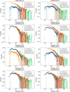 |
Fig. 10 Effective area comparison of GECAM and Fermi/GBM. |
Selected detectors for effective area comparison of GECAM-B and Fermi/GBM.
Spectral fitting results of GRB 220511A.
Acknowledgements
This work is supported by the National Key R&D Program of China (Grant No. 2021YFA0718500), GECAM the National Natural Science Foundation of China (Grant Nos. 12273042, 12303045), the Science Foundation of Hebei Normal University (No. L2023B11) and the Strategic Priority Research Program of the Chinese Academy of Sciences (Grant No. XDB0550300, XDA30050000). The GECAM (Huairou-1) mission is supported by the Strategic Priority Research Program on Space Science of the Chinese Academy of Sciences (XDA15360000). We acknowledge the public data and software from Fermi/GBM and the software from Elisa.
Appendix A Cross-calibration information and available energy range
Incident angle of GRDs on GECAM-B.
Available energy range for the 25 GRDs on board GECAM-B.
References
- An, Z., Sun, X., Zhang, D., et al. 2022, Radiat. Detect. Technol. Methods, 6, 43 [Google Scholar]
- An, Z.-H., Antier, S., Bi, X.-Z., et al. 2023, arXiv e-prints [arXiv:2303.01203] [Google Scholar]
- Band, D., Matteson, J., Ford, L., et al. 1993, ApJ, 413, 281 [Google Scholar]
- Bissaldi, E., von Kienlin, A., Lichti, G., et al. 2009, Exp. Astron., 24, 47 [Google Scholar]
- Brownlee, J. 2019, Probability; Machine Learning Mastery (San Francisco, CA, USA) [Google Scholar]
- Chen, Y., Huang, J., Li, X., et al. 2020, Sci. Sin. Phys. Mech. Astron., 50, 129507 [Google Scholar]
- Feng, P.-Y., An, Z.-H., Zhang, D.-L., et al. 2024, Sci. China Phys. Mech. Astron., 67, 111013 [Google Scholar]
- Goldstein, A., Cleveland, W. H., & Kocevski, D. 2022, Fermi GBM Data Tools: v1.1.1, https://fermi.gsfc.nasa.gov/ssc/data/analysis/gbm [Google Scholar]
- Guo, D., Peng, W., Zhu, Y., et al. 2020, Sci. Sin. Phys. Mech. Astron., 50, 129509 [Google Scholar]
- He, J.-J., An, Z.-H., Peng, W.-X., et al. 2023, MNRAS, 525, 3399 [Google Scholar]
- Huang, Y., Shi, D., Zhang, X., et al. 2024, Res. Astron. Astrophys., 24, 104004 [Google Scholar]
- Li, X., Wen, X., An, Z., et al. 2022, Radiat. Detect. Technol. Methods, 6, 12 [Google Scholar]
- Liddle, A. R. 2007, MNRAS, 377, L74 [NASA ADS] [Google Scholar]
- Liu, Y. Q., Gong, K., Li, X. Q., et al. 2022, Radiat. Detect. Technol. Methods, 6, 70 [Google Scholar]
- Luo, Q., Liao, J.-Y., Li, X.-F., et al. 2020, J. High Energy Astrophys., 27, 1 [Google Scholar]
- Lv, P., Xiong, S., Sun, X., Lv, J., & Li, Y. 2018, J. Instrum., 13, P08014 [Google Scholar]
- Meegan, C., Lichti, G., Bhat, P., et al. 2009, ApJ, 702, 791 [NASA ADS] [CrossRef] [Google Scholar]
- Qiao, R., Guo, D.-Y., Peng, W.-X., et al. 2024, Res. Astron. Astrophys., 24, 104005 [Google Scholar]
- Sakamoto, T., Pal’Shin, V., Yamaoka, K., et al. 2011, PASJ, 63, 215 [Google Scholar]
- Stamatikos, M. 2009, arXiv e-prints [arXiv:0907.3190] [Google Scholar]
- Sun, H., Wang, C.-W., Yang, J., et al. 2025, Natl. Sci. Rev., 12, nwae401 [Google Scholar]
- Tierney, D., McBreen, S., Hanlon, L., et al. 2011, AIP Conf. Proc., 1358, 397 [Google Scholar]
- Von Kienlin, A., Briggs, M., Connoughton, V., et al. 2009, AIP Conf. Proc., 1133, 446 [Google Scholar]
- Von Kienlin, A., Meegan, C. A., Paciesas, W. S., et al. 2014, ApJS, 211, 13 [Google Scholar]
- Wang, C. W., Xiong, S. L., Zhang, Y. Q., et al. 2022, ATel, 15682 [Google Scholar]
- Xiao, S., Xiong, S., Zhang, S., et al. 2021, ApJ, 920, 43 [Google Scholar]
- Xiao, S., Liu, Y., Peng, W., et al. 2022a, MNRAS, 511, 964 [NASA ADS] [CrossRef] [Google Scholar]
- Xiao, S., Xiong, S.-L., Cai, C., et al. 2022b, MNRAS, 514, 2397 [Google Scholar]
- Xiao, S., Zhang, S.-N., Xiong, S.-L., et al. 2024a, MNRAS, 528, 1388 [Google Scholar]
- Xiao, S., Hong, M.-X., You, Z.-Y., et al. 2024b, ApJS, 274, 14 [Google Scholar]
- Xiao, S., Li, X.-B., Xue, W.-C., et al. 2024c, MNRAS, 527, 11915 [Google Scholar]
- Xie, S.-L., Cai, C., Yu, Y.-W., et al. 2025, ApJS, 277, 5 [Google Scholar]
- Xu, Y., Li, X., Sun, X., et al. 2022, Radiat. Detect. Technol. Methods, 6, 53 [Google Scholar]
- Yi, S. X., Wang, C. W., Shao, X., et al. 2025, ApJ, 985, 239 [Google Scholar]
- Zhang, D., Li, X., Xiong, S., et al. 2019, Nucl. Instrum. Methods Phys. Res. A, 921, 8 [Google Scholar]
- Zhang, D., Sun, X., An, Z., et al. 2022a, Radiat. Detect. Technol. Methods, 6, 63 [Google Scholar]
- Zhang, D., Li, X., Wen, X., et al. 2022b, Nucl. Instrum. Methods Phys. Res. A, 1027, 166222 [Google Scholar]
- Zhang, D.-L., Zheng, C., Liu, J.-C., et al. 2023a, Nucl. Instrum. Methods Phys. Res. A, 1056, 168586 [Google Scholar]
- Zhang, Y.-Q., Xiong, S.-L., Qiao, R., et al. 2023b, arXiv e-prints [arXiv:2303.00698] [Google Scholar]
- Zhang, Y.-Q., Xiong, S.-L., Mao, J.-R., et al. 2024, Sci. China Phys. Mech. Astron., 67, 289511 [Google Scholar]
- Zhao, H.-S., Li, D., Xiong, S.-L., et al. 2023a, Sci. China Phys. Mech. Astron., 66, 259611 [NASA ADS] [CrossRef] [Google Scholar]
- Zhao, Y., Liu, J. C., Xiong, S. L., et al. 2023b, GRL, 50, e2022GL102325 [Google Scholar]
- Zhao, Y., Xue, W.-C., Xiong, S.-L., et al. 2023c, ApJS, 265, 17 [Google Scholar]
- Zhao, X.-Y., Xiong, S.-L., Wen, X.-Y., et al. 2024, Res. Astron. Astrophys., 24, 104002 [Google Scholar]
- Zheng, C., Peng, W., Li, X., et al. 2022, Nucl. Instrum. Methods Phys. Res. A, 167427 [Google Scholar]
- Zheng, C., Zhang, Y.-Q., Xiong, S.-L., et al. 2024a, ApJ, 962, L2 [Google Scholar]
- Zheng, C., An, Z.-H., Peng, W.-X., et al. 2024b, Nucl. Instrum. Methods Phys. Res. A, 1059, 169009 [Google Scholar]
- Zheng, C., Xiong, S., Li, C., et al. 2025, Sci. China Phys. Mech. Astron., 68, 271011 [Google Scholar]
All Tables
All Figures
|
Fig. 1 Schematic diagram of the installation position of the GRDs in GECAM. |
| In the text | |
|
Fig. 2 Cross-calibration process. |
| In the text | |
|
Fig. 3 Schematic diagram of spectra without fitting. The black and red dots represent the high-gain and the low-gain data, respectively, while the black and red lines correspond to the ideal net deposited count spectra for the High-Gain and the Low-Gain channels. |
| In the text | |
|
Fig. 4 Deposited counts spectra of the GRD01 detector in high-gain (top) and low-gain (bottom) channels. |
| In the text | |
|
Fig. 5 Joint fitting result of GRB 210606B with Fermi/GBM and GECAM in the Cuttoffpl model. |
| In the text | |
|
Fig. 6 Comparison of spectral fitting results: Fermi/GBM only vs. joint Fermi/GBM and GECAM-B. The black dashed line denotes the one-to-one correlation. Different colors indicate different spectral models, and each data point corresponds to an individual GRB. |
| In the text | |
|
Fig. 7 Constant of GECAM-B detectors with the high and low gains bound together. |
| In the text | |
|
Fig. 8 Fitting constant of GECAM-B detectors with the high and low gains separated. |
| In the text | |
|
Fig. 9 Relationship between constant factors and GRB’s flux. |
| In the text | |
|
Fig. 10 Effective area comparison of GECAM and Fermi/GBM. |
| In the text | |
Current usage metrics show cumulative count of Article Views (full-text article views including HTML views, PDF and ePub downloads, according to the available data) and Abstracts Views on Vision4Press platform.
Data correspond to usage on the plateform after 2015. The current usage metrics is available 48-96 hours after online publication and is updated daily on week days.
Initial download of the metrics may take a while.