| Issue |
A&A
Volume 701, September 2025
|
|
|---|---|---|
| Article Number | A189 | |
| Number of page(s) | 12 | |
| Section | Astrophysical processes | |
| DOI | https://doi.org/10.1051/0004-6361/202555299 | |
| Published online | 12 September 2025 | |
The NICER view of Scorpius X-1
1
Aurora Technology for the European Space Agency, ESAC/ESA, Camino Bajo del Castillo s/n, Urb. Villafranca del Castillo, Spain
2
Departament d’Astronomía i Astrofísica, Universitat de València, Dr. Moliner 50, 46100 Burjassot (València), Spain
3
INAF–Osservatorio Astronomico di Brera, Via E. Bianchi 46, 23807 Merate (LC), Italy
4
Department of Physics, Astrophysics, University of Oxford, Denys Wilkinson Building, Keble Road, OX1 3RH Oxford, UK
5
International Centre for Radio Astronomy Research–Curtin University, GPO Box U1987 Perth, WA 6845, Australia
6
Eureka Scientific, Inc., 2452 Delmer Street, Oakland, CA 94602, USA
7
Serco for the European Space Agency, ESAC/ESA, Camino Bajo del Castillo s/n, Urb. Villafranca del Castillo, Spain
⋆ Corresponding author: This email address is being protected from spambots. You need JavaScript enabled to view it.
Received:
25
April
2025
Accepted:
28
July
2025
Abstract
Context. The neutron star X-ray binary Scorpius X-1 is one of the brightest Z-type sources in our Galaxy, showing frequent periods of flaring activity and different types of relativistic outflows. Observations with RXTE have shown that the strongest X-ray variability appears in the transition to and from the flaring state. During this transition, it has been proposed that the appearance of two particular types of quasi-periodic oscillations (QPOs) might be connected with the ejection of the so-called ultra-relativistic flows.
Aims. In this paper, we present an analysis of the first NICER observations of Scorpius X-1 obtained during a multi-wavelength campaign conducted in February 2019, in order to characterise the properties of QPOs in this source as the system evolves through its various accretion states.
Methods. We computed a light curve and a hardness-intensity diagram to track the evolution of the source spectral properties, while we investigated the X-ray time variability with a dynamical power density spectrum. To trace the temporal evolution of QPOs, we segmented the dataset into shorter, continuous intervals, and computed and fitted the averaged power density spectrum for each interval.
Results. Our analysis shows that the overall behaviour of the source is consistent with the literature; strong QPOs around 6 Hz are detected on the normal branch, while transitions to and from the flaring branch – occurring over timescales of a few hundred seconds – are characterised by rapid, weaker quasi-periodic variability reaching frequencies up to 15 Hz. Despite limited statistical significance, we also identify faint, transient timing features above 20 Hz, which occasionally coexist with the prominent 6 Hz QPOs. Although tentative, the existence of these timing features in the NICER data is crucial for interpreting the simultaneous radio observations from the same multi-wavelength campaign, potentially reinforcing the connection between the ejection of relativistic outflows and the accretion states in Scorpius X-1.
Key words: binaries: general / stars: jets / stars: neutron
© The Authors 2025
 Open Access article, published by EDP Sciences, under the terms of the Creative Commons Attribution License (https://creativecommons.org/licenses/by/4.0), which permits unrestricted use, distribution, and reproduction in any medium, provided the original work is properly cited.
This article is published in open access under the Subscribe to Open model. This email address is being protected from spambots. You need JavaScript enabled to view it. to support open access publication.
1. Introduction
Neutron star low-mass X-ray binaries (NS LMXBs) are stellar binary systems in which the compact object (CO; the accretor) is a NS orbiting a low-mass companion (the donor). Based on their spectral and timing properties, they are classified into two main categories: Z-type sources and atoll-type sources (Hasinger & van der Klis 1989), depending on the characteristic shape that NS LMXBs trace in the X-ray colour-colour diagram (CD) or in the hardness-intensity diagram (HID). In particular, Z-type sources are the most luminous, accreting near or above the Eddington rate. In the aforementioned diagrams, they draw a characteristic Z-like shape where we can distinguish three separate branches: the horizontal branch (HB), the normal branch (NB), and the flaring branch (FB). A hard apex (HA) separates the HB and the NB, and a soft apex (SA) separates the NB and the FB. These branches represent specific accretion states of the system, which may be crossed on short (hours or less) timescales (Muñoz-Darias et al. 2014). Moreover, all known Z-type NS LMXBs are persistent radio-emitting sources.
The radio luminosity of Z-source varies as a function of the state in the CD or HID (Penninx et al. 1988; Hjellming et al. 1990a,b), which is stronger on the HB (or high NB), and quenched in the FB (or low NB). This variability is physically connected to specific changes in the accretion flow, similar to the disc-jet coupling observed in LMXBs hosting a stellar-mass black hole (BH; e.g. Migliari & Fender 2006).
The power density spectrum (PDS) of Z-type NSs also changes from one accretion state to another (i.e. Méndez et al. 1999), showing different types of quasi-periodic oscillations (QPOs) that can be classified into two main categories: kilohertz QPOs, detected isolated or in pairs above 500 Hz (i.e. van der Klis 1989), and low-frequency (LF) QPOs, typically appearing below 50 Hz. The latter are further divided into three different types, depending on the branch of the CD or HID where they manifest (e.g. van der Klis 1989): horizontal branch oscillations (HBOs), normal branch oscillations (NBOs), and flaring branch oscillations (FBOs). These are considered to be the NS equivalent of the so-called type C, type B, and type A QPOs found in BH systems (Ingram & Motta 2019).
The X-ray binary (XRB) Scorpius X-1 (hereafter, Sco X-1) was discovered in 1962 (Giacconi et al. 1962) and is the brightest extrasolar X-ray source in the sky, located at a distance of 2.33 kpc (Gaia Collaboration 2021). It is classified as a LMXB with an orbital period of 18.9 h (Gottlieb et al. 1975), containing a later-than-K4 spectral type companion star (0.28 M⊙ < M < 0.70 M⊙) and a weakly magnetised NS with a mass of < 1.73 M⊙ (Mata Sanchez et al. 2015). Sco X-1 is one of a select number of permanent Z-type sources in our Galaxy (together with GX 349+2, GX 340+0, GX 17+2, GX 5-1, Cyg X-2, GX 13+1, and the peculiar system Cir X-1), and it is known to show extended radio luminous jets (i.e. radio lobes; Fomalont et al. 2001a).
Over the past few decades, several X-ray observations of Sco X-1 have investigated the timing properties of the source (see e.g., Titarchuk et al. 2014, and references therein). Using EXOSAT, Middleditch & Priedhorsky (1986) first discovered a 6 Hz QPO, which was later shown to vary from 10 to 20 Hz on short timescales during an active state (Priedhorsky et al. 1986; van der Klis et al. 1987; Dieters & van der Klis 2000). van der Klis et al. (1996) reported the discovery of 45 Hz QPOs in the RXTE data, besides (sub)millisecond oscillations (the so-called kilohertz QPOs), correlated with the frequency of the 6–20 Hz QPOs in the NB to FB transition. Some years later, Casella et al. (2006) showed the first resolved rapid transition from a FBO to an NBO, with a monotonic (smooth) increase in the QPO centroid frequency from 4.5–7 Hz (in the NB) to 6–25 Hz (in the FB).
In the radio band, Fomalont et al. (2001a) showed that the radio structure of Sco X-1 is composed of a radio core and two symmetric radio lobes. In Fomalont et al. (2001b), the authors suggested for the first time the existence of relativistic flows travelling along the jets – later dubbed ultra-relativistic flows (URFs) – inferred by correlating X-ray flares in the core with subsequent radio flares in the approaching and receding lobes. This type of fast flow, whose origin and physical properties are still unclear, has also been observed in at least two other XRBs; namely, Cir X-1 (Fender et al. 2004; Tudose et al. 2008, but see also Miller-Jones et al. 2012) and SS 433 (Migliari et al. 2005, but see also Miller-Jones et al. 2008). More recently, Motta & Fender (2019) re-analysed the RXTE data of Sco X-1 and suggested that this type of outflow is related to the appearance of a particular class of QPO, while radio-emitting outflows are associated with flat-top broad-band noise components. In particular, the authors found evidence that URF ejections occur when both an NBO and an HBO are present in the X-ray power spectrum. This might indicate, at least tentatively, that the ejection of URFs is connected with specific changes in the accretion flow.
From 21 to 25 February 2019, an extensive multi-wavelength campaign was organised to monitor Sco X-1 with different instruments, providing the largest simultaneous coverage at all possible wavelengths with radio/VLBI (VLBA + EVN + LBA, rotating through each array as the Earth rotated, to provide continuous coverage), radio/VLA, optical/IR (SALT, VLT, NOT and TNG), X-ray (NICER, Chandra, XMM-Newton), and γ-ray (INTEGRAL) observations. In the X-ray energy range, the large collecting area of the NICER observatory (Gendreau et al. 2012), together with its ability to handle very high count rates, provided the highest-quality data of the X-ray instruments involved in the campaign.
In this paper, we present an analysis of the timing properties of Sco X-1 using NICER observations performed during the February 2019 multi-wavelength campaign. We mainly focus on the different types of LF QPOs that appear in the dataset, and on how the characteristics of these QPOs (especially the central frequency) change along the position in the HID. This constitutes the first comprehensive analysis of Sco X-1 based on NICER X-ray observations.
The paper is organised as follows. In Sect. 2, we describe the NICER observations and the methodology we follow to produce a light curve, the HID, and the (dynamical) PDS. In Sect. 3, we present the main results of the timing analysis. Finally, in Sect. 4, we discuss our results and we draw our main conclusions.
2. Observations and data analysis
2.1. MAXI
We first produced a light curve and a HID using MAXI data taken from 1 February 2019 to 31 March 2019 (from 58515 to 58573 MJD), using the MAXI/GSC on-demand web interface1 (Matsuoka et al. 2009). We analysed data extracted within a circular region with a radius of 1.6° around the source position (244.979455, −15.640283), while the background region was extracted in a concentric ring with an outer radius of 3°. The bin size is 1 hour (i.e. 0.04 days). Light curves were extracted in two energy bands: 2–10 keV (A) and 10–20 keV (B), and the hardness ratio (HR) was defined as HR = B/A.
2.2. NICER
The NICER dataset is composed of three different observations, identified by proposal numbers 110803010 (Obs-1; from 58536.450 to 58536.978 MJD), 1108030111 (Obs-2; from 58537.026 to 58537.940 MJD), and 1108030112 (Obs-3; from 58537.991 to 58538.777 MJD). For each observation, we used the unfiltered merged measurement/power unit science data (available under the path /xti/event_cl/) and performed the standard cleaning using the high-level screening task NICERCLEAN (Heasoft v6.28). Data analysis (including light curve and PDS extraction) was performed using the general high-energy aperiodic timing software (GHATS)2. This software, which is an interactive timing package working on IDL/GDL, has been extensively validated for X-ray timing with RXTE and other missions, including NICER observations (see e.g., Belloni et al. 2005, 2024; Motta et al. 2017; Motta & Fender 2019; Bhargava et al. 2019; López-Miralles et al. 2023).
2.2.1. Light curve and hardness-intensity diagram
We produced a light curve and a HID with a time bin resolution of 13 s. Time gaps were removed from the data, as well as instrumental drops at the beginning of each segment. We extracted the count rate in the energy bands A =[0.5 − 2] keV and B =[2 − 15] keV, and we defined the HR as HR = B/A. The HID was produced by plotting the HR against the intensity (i.e. the accumulated count rate in the two energy bands, A + B).
2.2.2. (Dynamical) power density spectra
We re-binned the NICER high-resolution Science mode data in time (×104) to obtain a Nyquist frequency of 1250 Hz. Using fast Fourier transform techniques (van der Klis 1989), we produced PDSs for continuous 13 s-long intervals and averaged them to obtain a PDS for the whole dataset (including the three observations). We show this PDS in the traditional ν, Pν representation, where we applied the Leahy normalisation (Leahy et al. 1983). The PDSs were fitted with the XSPEC package using a one-to-one energy-frequency conversion and a unity response matrix. This allowed us to fit a power versus frequency spectrum as if it was a flux versus energy spectrum. Throughout this work, we always consider a multi-Lorentzian model plus a power law component to take into account the contribution of the Poisson noise (see e.g., Belloni et al. 2002). To show how the PDS changes with time, we also computed a dynamical PDS following similar techniques (Pν in the time vs frequency plane).
To search for fainter and/or short-lived timing features, we divided the whole dataset into continuous shorter segments, taking advantage of the location of the light-curve gaps. For each of these segments, we produced a collection of PDSs by averaging 30 consecutive 13 s-long bins (i.e. 390 s), covering the total time length of the three observations. Before averaging, PDS sets containing fewer than 15 bins were automatically discarded. In an attempt to increase the strength of the variability, for this part of the analysis we also removed photons in the energy range below 750 eV.
2.3. XMM-Newton: The brightest observation ever
XMM-Newton observed Sco X-1 between 21 February 2021 and 22 February 2021 for a total exposure time of approximately 100 ks (rev. 3517, ObsId 0831790901). The EPIC-pn camera was operated in burst mode with the THIN filter, resulting in the highest count rate ever measured with the XMM-Newton observatory (above 7 × 10⁴ counts/s). However, this extraordinarily high rate, which was above the operational limits of the EPIC-pn instrument, led to multiple resets due to the extremely high workload of the on-board electronics (FIFO overflows), besides the quasi-periodic triggering of the so-called counting mode due to telemetry saturation (with an activation period of approximately 18 s). As a result, the timing information in the science files was corrupted, both in terms of integration time for spectral products and of GTI correction of rates in the resulting light curves. Therefore, we concluded that the XMM-Newton data taken during February 2019 is not appropriate for timing studies of Sco X-1, and we have not considered it in this paper.
3. Results
Figure 1 shows the MAXI light curve coloured by the HR (A + B, in units of counts; top) and the HID coloured by time in MJD (B/A vs. A + B; bottom). The light curve shown in Fig. 1 (top) reveals that the source experiences frequent flaring activity during the two months of MAXI continuous monitoring, where the HID (bottom) shows the characteristic pattern of a NS Z-source, with a FB, a NB, and a HB (from top to bottom). In both panels, data collected simultaneously with NICER during the February 2019 multi-wavelength monitoring (from 58536.4 to 58538.7 MJD) is represented with star markers. This small subset of points (∼1 h time bins) shows two distinct important incursions into the FB: the first one at 58536.7 MJD and the second one at 58538.6 MJD. However, the information provided by the light curve in this time range is limited, since no MAXI observations were collected from 58536.7 to 58538.4 MJD.
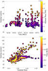 |
Fig. 1. Light curve (top) and HID (bottom) of Sco X-1 using MAXI data taken from 1 February 2019 to 31 March 2019 with a time resolution of 0.04 days. The light curve is colour-coded with the HR = B/A, and the HID with the time (in MJD). Data taken from 22 February 2019 to 24 February 2019, corresponding to the multi-wavelength campaign, are represented with star markers. |
The NICER light curve of Fig. 2 shows these two big flares with much more time resolution, where the x axis corresponds to the relative time after removing all time gaps and instrumental drops, and the colour map represents the HR as defined in Sect. 2.2.1. Figs. 3–4 show, respectively, the HID for the full dataset and for each individual observation.
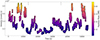 |
Fig. 2. Light curve (in units of counts/s) for the full dataset after removing time gaps and instrumental drops. The two division marks at the top of the plot separate the three NICER observations. The colour scale represents the HR as defined in Sect. 2.2.1. |
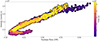 |
Fig. 3. Hardness-intensity diagram for the entire dataset. The colour scale represents the relative time in seconds after removing time gaps and instrumental drops (as shown in the x axis of Fig. 2). The two division marks in the colour bar show the limit of each NICER observation. |
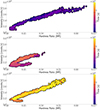 |
Fig. 4. Same as Fig. 3 for Obs-1 (top), Obs-2 (middle), and Obs-3 (bottom). In each panel, the time in the colour bar corresponds to the total relative time of the full dataset displayed in the x axis of Fig. 2. |
During the flaring state, the source is highly variable, showing rapid transitions back and forth. It is also interesting to note that, despite the main flares showing approximately the same count rate (∼28 000 counts/s), the HR is higher during the first incursion into the FB. In the HID of Fig. 3, this creates a fish-hook-like pattern in the top part of the branch, with a harder – and longer – branch corresponding to the first burst, and a softer branch corresponding to the second one. In the NICER data, the NB is generally not well resolved, and the transition to the HB can only be slightly deduced in Obs-2 (see Fig. 4, central plot).
The averaged PDS shown in Fig. 5 is dominated by a ∼6 Hz QPO, revealing low-frequency red noise below 1 Hz and flat-top noise above this frequency (aside from the QPO). As is described in Sect. 2.2.2, we fitted the PDS with a five-Lorentzian model plus a power-law component to account for the contribution of the Poisson noise. Using this model, the central frequency of the QPO yields 6.35 ± 0.06 Hz (χν2 = 176/156). This feature is the by-product of the strong variability shown in the dynamical PDS of Fig. 6 (in yellow-white), which also shows weaker variability in the 6–20 Hz frequency range. The strongest variability signal appears when the source is in the quiet state (near the light-curve minima at 2 × 10⁴ counts/s), while rapid – and fainter – variability up to 20 Hz precedes and follows the source flaring activity (> 2.2 × 10⁴ counts/s).
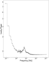 |
Fig. 5. Power density spectrum for the entire NICER dataset, including Obs-1, Obs-2, and Obs-3. Broad-band red-noise appears below ∼30 Hz, while a strong QPO is observed at 6.35 ± 0.06 Hz. At higher frequencies, power is dominated by Poisson noise. |
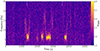 |
Fig. 6. Dynamical PDS for the entire NICER dataset, including Obs-1, Obs-2, and Obs-3. The plot shows a strong signal below 10 Hz and weaker fast variability between 10 Hz and 20 Hz. The two division marks at the top of the plot separate the three NICER observations. |
In order to characterise these transitions along the HID, in the rest of this section we report the results of the analysis described in the second paragraph of Sect. 2.2.2. For this purpose, we have computed averaged PDS every ∼400 s, which were fitted with a multi-Lorentzian+power-law statistical model in XSPEC. As is described in Appendix A, each PDS is defined with a unique token that identifies the PDS number, the light-curve segment (i.e. the continuous chunks of data between light-curve gaps) and the position of the PDS in the segment, in this order.
In this paper, we assume the following convection to claim a QPO discovery: we consider narrow features (Q > 2, where Q is the QPO quality factor3) with sufficient statistical significance (3σ), although a few exceptions to this rule are also considered. On the one hand, when the Q-factor is Q ≤ 2 and the statistical significance is > 3σ, QPOs are referred to as ‘broad’ or ‘blurred’ features. On the other hand, when the statistical significance is ≤3σ but Q > 2, QPOs are referred to as ‘faint’ narrow features. This nomenclature is relevant to follow the dynamical evolution of the statistically significant QPOs in this source, while providing evidence of the existence of other features that are difficult to resolve in our dataset. The results of the analysis for each individual PDS are reported in the tables of Appendix A.
3.1. Observation 1 (110803010)
The main characteristics of the QPOs found in Obs-1 (central frequency, Q-factor, and statistical significance in sigmas) are displayed on Table 1. In this first observation, the source spends most of the time in the FB, showing several transitions from the low FB to the high FB. As is shown in the dynamical PDS of Fig. 6, no relevant aperiodic variability is expected during this state, and the PDSs are mostly dominated by broad-band noise. The strongest signal appears on segment #08 (see Table A.1), when the source moves from the FB towards the NB. This transition is characterised by the presence of a well-resolved FBO, which decreases in frequency as the source approaches the SA. In some of the PDSs of the last segment (#290800, #320803), we observe a second component at lower frequencies, possibly due to changes of the FBO frequency on short timescales (this second component was, however, difficult to constrain in the model due to low signal-to-noise at these low frequencies).
Statistical parameters of the QPOs discovered in Obs-1.
Besides the LF QPOs near the SA, in two PDS distributed along the FB (i.e. #010001, #070202) we also found very narrow QPO-like features in the frequency range between 30 Hz and 40 Hz (see Table A.1). Although these features are statistically significant according to the adopted convention (i.e. > 3σ), these narrow QPOs were difficult to constrain in the models so we do not report them as part of the main findings of Table 1.
3.2. Observation 2 (110803011)
The main characteristics of the QPOs found in Obs-2 are shown in Table 2. This NICER observation shows high variability, where approximately half of the PDS reveal some kind of QPO feature. The three PDSs of segment #00 are dominated by a strong NBO (with a statistical significance of > 12σ), which shifts slightly in frequency from 6.34 Hz (PDS #000000) to 7.67 Hz (PDS #020002) as the source moves from the NB towards the SA (see also Table A.2).
Statistical parameters of the QPOs discovered in Obs-2.
In this observation, we can distinguish two main incursions into the FB; the first in segment #01 (t ∼ 18 000 s in the light curve of Fig. 2) and the second one in segment #10 (t ∼ 32 000 s in the light curve of Fig. 2). There is also a fast transition into the low-FB in segment #07, where the dynamical PDS shows rapid back-and-forth variability in the frequency range from 6 to 20 Hz (see Fig. 6). The first incursion into the FB is characterised by the presence of an FBO in the first PDS of segment #01 (with central frequency 13.6 Hz), which is the consequence of the shift of the NBO of segment #00 towards higher frequencies. In the FB, PDS show broad-band noise components with no aperiodic features. On segment #04, the flaring activity ceases and the source returns to the NB, where NBOs reappear. As the HR increases and the source moves towards the HA, the NBO smears in the PDS noise. On segment #05, the source is in the HA, where we could resolve a single isolated HBO at 33.65 Hz (Q∼ 9 and 3.7σ), which is the only example of this type of QPO that we could find in the whole NICER dataset. Every other attempt to fit an HBO-like feature resulted in very low statistical significance (see e.g. PDS #00000 and PDS #180600 in Table 2). However, given the importance of this kind of QPO for the purposes of this paper, we report our results even when the statistics are not formally relevant.
When the source again moves towards the SA, the strong NBO reappears. In segment #07, the source shows a rapid incursion into the low FB that triggers an FBO in the frequency range 14–17 Hz, which turns back into a strong NBO when the source returns to the NB in segment #08 and segment #09. From segment #10 onwards, the source moves into the FB and the FBOs are detected again in the PDS, despite the source being in the mid-low FB state (see e.g. PDS #361200 in Table A.2).
3.3. Observation 3 (110803012)
The main characteristics of the QPOs found in Obs-3 are shown in Table 3. In this observation, the source is predominantly active (as it is in the case of Obs-1), showing two main incursions into the NB: the first one in segment #01 (t ∼ 43 000 s in the light curve of Fig. 2), and the second one at the end of the observation, in segment #12 (t ∼ 52 000 s in the light curve of Fig. 2).
Statistical parameters of the QPOs discovered in Obs-3.
During the first incursion, three PDSs show strong NBOs at ∼6 Hz (PDS #030100, PDS #040101, and #PDS 050102). In PDS #040101, we fitted a second component above 20 Hz, for which we got a borderline detection with low statistical significance (2σ). This corresponds to the higher significance that we could get in the three observations when attempting to fit an HBO-like component together with the strong NBOs at 6 Hz.
In PDS #060200, a blurred FBO (Q = 0.9) at ∼9 Hz marks the transition from the NB to the FB. During the flaring state, PDS are dominated by broad-band noise, but we also detected three FBO features in PDS #110302, PDS #160600, and PDS #230801. The last three PDSs of the dataset (#341200, #351201, and #361202) represent the second transition to the NB and the end of the flaring state. These PDS are characterised by well-resolved FBOs above 14 Hz.
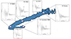 |
Fig. 7. Fiducial PDS for different spectral states in the HID of Fig. 3. Bigger panels with pink stars show the main timing features observed in the NICER dataset: the NBOs in the NB (PDS #010001 of Obs-2), the FBOs in the transition from the NB to the FB (PDS #220701 of Obs-2), the isolated HBO near the HA (PDS #150500 of Obs-2), and the broad-band red noise observed in the FB (PDS #130401 of Obs-3). The two smaller panels with grey stars show less common and tentative features, such as the narrow QPOs discovered in the mid FB (PDS #010001 of Obs-1), or the pair NBO + HBO in the NB (PDS #040101 of Obs-3). |
4. Discussion
In this paper, we present the analysis of the X-ray fast time variability properties of the NS LMXB Sco X-1 as observed by NICER. This monitoring is part of a large multi-wavelength campaign performed on Sco X-1 over almost four full days in February 2019, when NICER provided the highest-quality data among all the X-ray instruments.
We considered three NICER observations for a total exposure of ∼55 ks, each of which was split into continuous shorter segments, taking advantage of the light-curve gaps. In each of these segments, we computed averaged PDSs by stacking 13 s long bins every ∼400 s.
Approximately half of the 115 PDS we inspected show some kind of QPO feature, while the rest are dominated by broad-band noise components. We observed the following: 20 PDSs containing NBOs, 20 PDSs showing FBOs, and 1 PDS showing a statistically significant HBO (plus 1 faint detection in Obs-3). We also observed at least another distinct type of QPO that is more difficult to classify according to the above categories, which appeared during the flaring state with no obvious preferential location in the FB. These features are the three narrow QPOs detected in the frequency range 30–40 Hz in Obs-1 and Obs-2 (see Tables A.1–A.2), and above 60 Hz in Obs-3 (see Table A.3). Although these features are marginally significant and difficult to constrain in the models (so they might correspond to spurious variability), we briefly discuss them in this section.
In order to draw a coherent picture of the source behaviour, Fig. 7 summarises the quasi-periodic variability content of the data in the framework of the HID. In the figure, we show a strong 6 Hz NBO (sub-panel (a), PDS #010001 of Obs-2, see Table A.2), an FBO during the transition to the FB (sub-panel (b), PDS #220701 of Obs-2, see Table A.2), a narrow QPO-like feature appearing during the flaring state (sub-panel (c), PDS #010001 of Obs-1, see Table A.1), broad-band red noise (sub-panel (d), PDS #130401 of Obs-3, see Table A.3), the only isolated HBO that we found in our analysis (sub-panel (e), PDS #150500 of Obs-2, see Table A.2), and the tentative pair NBO + HBO found in the NB, where the HBO is not statistically significant and thus it is only classified as a faint detection (sub-panel (f), PDS #040101 of Obs-3, see Table A.3).
4.1. Normal-to-flaring branch transitions
The overall behaviour of the source is consistent with what has been reported in the literature. The PDSs in the NB are characterised by strong NBOs at ∼6 Hz (first discovered by Middleditch & Priedhorsky 1986), while all display broad-band red noise as the source moves along the FB. As is shown in the dynamical PDS of Fig. 6, the transition from the NB to the FB is distinguished by the shift of the NBO towards higher frequencies (or by the shift of the FBO towards lower frequencies in the inverse transition, see e.g. Priedhorsky et al. 1986; van der Klis et al. 1987; Dieters & van der Klis 2000; Casella et al. 2006), while NBOs disappear as the source moves towards the HA (see e.g. PDS #140402 in Table A.2). As is shown in Fig. 8, the timescale at which this transition takes place is of the order of a few hundred seconds, in agreement with the results reported in the literature for RXTE (Casella et al. 2006).
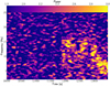 |
Fig. 8. Dynamical PDS for segments #07 and #08 of Obs-1. A smooth FB-to-NB transition is resolved in segment #08. This corresponds to the unique transition that is fully resolved within one single segment, as all other examples in Obs-2 and Obs-3 coincide with a data gap. The signal smoothly decreases from 15 Hz to 6 Hz in a few hundred seconds. |
We have found tentative evidence that these transitions might also occur at a much higher rate. This is suggested, for example, by the presence of a statistically significant QPO observed in PDS #230801 of Obs-3 (see Table A.3). We classified this QPO as an FBO because it is located in the mid FB, but its central frequency is fully compatible with the strong NBOs of the source, which are lower than the characteristic frequency of the FBOs appearing during the transition to and from the flaring state. Thus, we speculate that the presence of this QPO in the FB may indicate a very rapid excursion of the source into the NB, faster than the typical timescales of the spectral transitions in Sco X-1.
4.2. Narrow QPOs in the flaring branch
The nature of the narrow QPOs detected in the FB above 30 Hz is unclear. The central frequency of these features varies from 30–40 Hz in Obs-1 and Obs-2, to > 60 Hz in Obs-3 (see one example in Fig. 7 for PDS #010001 of Obs-1). Similar features were observed in RXTE observations of Sco X-1 up to ∼70 Hz (Motta et al., in prep.). While appearing in the FB, these features show certain similarities with the HBOs seen at lower frequencies. Something similar occurs in BH systems, where type-C QPOs (the HBO equivalent in BHs) are observed in the soft state (see e.g. Motta et al. 2012; Franchini et al. 2017). The features we observed in the FB might thus be related to the HBOs seen in the HB. In particular, as has been noted in the literature (see Stella & Vietri 1998; Motta et al. 2017), such features could be the second harmonic of an undetected fundamental frequency. However, the small number of events, together with the marginal significance of these detections and the difficulty of constraining the properties of such narrow, low-amplitude features, limit the robustness of any conclusion that we could draw about their nature. Therefore, based on the available data, we cannot exclude the possibility that these features are spurious detections.
4.3. Horizontal branch oscillations and URFs
Given its tentative connection with the ejection of URFs, the existence of HBOs – especially together with an NBO – should be carefully addressed. The fact that NBO + HBO pairs are less common in the NICER dataset than in RXTE (Motta & Fender 2019) is to be expected. Due to the soft response of the NICER detector (0.1–10 keV), HBOs are harder to detect compared to, for instance, the PCA instrument on board RXTE, which reached up to 40 keV. Nevertheless, given the relevance of HBOs in the study of relativistic ejections in Sco X-1, along with the existence of an isolated HBO resolved at 34 Hz, we decided to report in this work any aperiodic feature that shows in this frequency range, even if it is not formally statistically significant. It is important to note that, aside from NICER, no other X-ray instrument provides a time resolution high enough to assess this frequency range, so this information – although tentative – may be relevant for comparison with the radio observations of Sco X-1.
These faint HBO-like features seem to be present together with NBOs in Obs-2 and Obs-3 above 20 Hz, with a maximum significance of 2σ in PDS #040101 of Obs-3 (see blue numbers in Tables 2–3). Since we expect HBOs to be transient features, we have closely inspected the dynamical PDS of Fig. 6 in the segments where our analysis evidences such faint features at higher frequencies (together with an NBO). As is shown in Fig. 9, we observe some faint variability in segment #00 of Obs-2 above 20 Hz, which is compatible with the faint features reported in Tables 2–3 for the averaged PDS. We thus consider the existence of this transient fast variability in the dynamical PDS at the expected frequencies to provide more strength to the results discussed in this section.
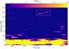 |
Fig. 9. Dynamical PDS for segment #00 of Obs-2. Transient fast variability is observed above 20 Hz (white box), together with the strong signal around 6 Hz. This variability is compatible with the features reported in Tables 2–3 for Obs-2 and Obs-3, respectively. |
In van der Klis et al. (1997) and Motta & Fender (2019), all HBOs show approximately the same central frequency (∼45 Hz), while in NICER these features seem to be more scattered at lower frequencies, ranging from 20 Hz (the faint detections coupled to NBOs) to 35 Hz (the single isolated HBO in Obs-3). Due to this fact, we question whether these borderline QPOs (especially the ones at lower frequencies, close to 20 Hz) could represent the sub-harmonic of an undetected fundamental oscillation, which may be submerged in the Poissonian noise at higher frequencies (see e.g. Motta et al. 2017). However, since HBOs are transient and may be short-lived (see Fig. 9), it is also possible that the characteristic frequency of the QPO varies over time in a wider frequency range. If this is the case, then the NICER characteristics (low or no sensitivity to high-energy photons) may be the reason why we do not observe these features at the expected higher frequencies.
Motta & Fender (2019) showed that the launch of relativistic jets in Sco X-1 is tightly connected with the appearance of certain specific timing features in the PDS of the source, and in particular of an NBO (or the type-B QPO in BH XRBs), generally considered the jet QPO (among others, see Migliari et al. 2005). Clearly, the fact that NBOs and type-B QPOs may be associated with jets is mostly circumstantial evidence, as the connection between such QPOs and the jet is still unclear and largely debated (as are the possible jet launching mechanisms).
Motta & Fender (2019) found that the ejection of the (invisible) URFs seems to be associated with the appearance of not only an NBO in the PDS, but also an HBO at the highest end of the frequency range spanned by such a feature. This implies that the accretion flow reaches as close as possible to the NS surface. Hence, the simultaneous appearance of the NBO + HBO pair indicates that not only an outflow was launched – an URF, as was deduced from the radio data – but that it is launched when the accretion flow is closest to the central NS. Such a configuration has long been speculated, but to date no better smoking gun has been found than the appearance of a NBO + HBO pair.
Although the statistics are poor, our results show that the tentative NBO + HBO PDSs we found in our data appear at the expected location in the HID, i.e. when the URF is expected to be launched based on Motta & Fender (2019). Interestingly, a preliminary analysis of the radio data taken as part of the same observing campaign shows a number of URF ejections (Motta et al., in prep.), all launched at times consistent with the appearance of the NBO + HBO. Therefore, despite the poor statistical significance of the NICER HBO + NBO detections, we argue that our findings provide further support – at least qualitatively – for the connection between the accretion event responsible for the appearance of NBO + HBO pairs, and the launch of URFs in Sco X-1.
We define the quality factor Q = ν0/2Δ, where ν0 is the central frequency of the QPO, and Δ is the half width at half maximum.
Acknowledgments
The project that gave rise to these results received the support of a fellowship from “La Caixa” Foundation (ID 100010434). The fellowship code is LCF/BQ/DR19/11740030. J.L.M acknowledges additional support from MICIU/AEI/10.13039/501100011033 and from Ministerio de Ciencia e Innovación (MCIN) within the Plan de Recuperación, Transformación y Resiliencia del Gobierno de España through the project ASFAE/2022/005.
References
- Belloni, T., Psaltis, D., & van der Klis, M. 2002, ApJ, 572, 392 [NASA ADS] [CrossRef] [Google Scholar]
- Belloni, T., Homan, J., Casella, P., et al. 2005, A&A, 440, 207 [NASA ADS] [CrossRef] [EDP Sciences] [Google Scholar]
- Belloni, T. M., Méndez, M., García, F., & Bhattacharya, D. 2024, MNRAS, 527, 7136 [Google Scholar]
- Bhargava, Y., Belloni, T., Bhattacharya, D., & Misra, R. 2019, MNRAS, 488, 720 [NASA ADS] [CrossRef] [Google Scholar]
- Casella, P., Belloni, T., & Stella, L. 2006, A&A, 446, 579 [NASA ADS] [CrossRef] [EDP Sciences] [Google Scholar]
- Dieters, S. W., & van der Klis, M. 2000, MNRAS, 311, 201 [Google Scholar]
- Fender, R., Wu, K., Johnston, H., et al. 2004, Nature, 427, 222 [CrossRef] [Google Scholar]
- Fomalont, E. B., Geldzahler, B. J., & Bradshaw, C. F. 2001a, ApJ, 558, 283 [Google Scholar]
- Fomalont, E. B., Geldzahler, B. J., & Bradshaw, C. F. 2001b, ApJ, 553, L27 [NASA ADS] [CrossRef] [Google Scholar]
- Franchini, A., Motta, S. E., & Lodato, G. 2017, MNRAS, 467, 145 [Google Scholar]
- Gaia Collaboration (Brown, A. G. A., et al.) 2021, A&A, 649, A1 [NASA ADS] [CrossRef] [EDP Sciences] [Google Scholar]
- Gendreau, K. C., Arzoumanian, Z., & Okajima, T. 2012, in Space Telescopes and Instrumentation 2012: Ultraviolet to Gamma Ray, eds. T. Takahashi, S. S. Murray, & J.-W. A. den Herder, SPIE Conf. Ser., 8443, 844313 [CrossRef] [Google Scholar]
- Giacconi, R., Gursky, H., Paolini, F. R., & Rossi, B. B. 1962, Phys. Rev. Lett., 9, 439 [NASA ADS] [CrossRef] [Google Scholar]
- Gottlieb, E. W., Wright, E. L., & Liller, W. 1975, ApJ, 195, L33 [Google Scholar]
- Hasinger, G., & van der Klis, M. 1989, A&A, 225, 79 [NASA ADS] [Google Scholar]
- Hjellming, R. M., Han, X. H., Cordova, F. A., & Hasinger, G. 1990a, A&A, 235, 147 [Google Scholar]
- Hjellming, R. M., Stewart, R. T., White, G. L., et al. 1990b, ApJ, 365, 681 [Google Scholar]
- Ingram, A. R., & Motta, S. E. 2019, New Astron. Rev., 85, 101524 [Google Scholar]
- Leahy, D. A., Elsner, R. F., & Weisskopf, M. C. 1983, ApJ, 272, 256 [Google Scholar]
- López-Miralles, J., Motta, S. E., Migliari, S., & Jaron, F. 2023, MNRAS, 523, 4282 [Google Scholar]
- Mata Sanchez, D., Munoz-Darias, T., Casares, J., et al. 2015, MNRAS, 449, L1 [Google Scholar]
- Matsuoka, M., Kawasaki, K., Ueno, S., et al. 2009, PASJ, 61, 999 [Google Scholar]
- Méndez, M., van der Klis, M., Ford, E. C., Wijnands, R., & van Paradijs, J. 1999, ApJ, 511, L49 [Google Scholar]
- Middleditch, J., & Priedhorsky, W. C. 1986, ApJ, 306, 230 [NASA ADS] [CrossRef] [Google Scholar]
- Migliari, S., & Fender, R. P. 2006, MNRAS, 366, 79 [CrossRef] [Google Scholar]
- Migliari, S., Fender, R. P., Blundell, K. M., Méndez, M., & van der Klis, M. 2005, MNRAS, 358, 860 [NASA ADS] [CrossRef] [Google Scholar]
- Miller-Jones, J. C. A., Migliari, S., Fender, R. P., et al. 2008, ApJ, 682, 1141 [NASA ADS] [CrossRef] [Google Scholar]
- Miller-Jones, J. C. A., Moin, A., Tingay, S. J., et al. 2012, MNRAS, 419, L49 [NASA ADS] [Google Scholar]
- Motta, S. E., & Fender, R. P. 2019, MNRAS, 483, 3686 [Google Scholar]
- Motta, S., Homan, J., Muñoz Darias, T., et al. 2012, MNRAS, 427, 595 [NASA ADS] [CrossRef] [Google Scholar]
- Motta, S. E., Rouco Escorial, A., Kuulkers, E., Muñoz-Darias, T., & Sanna, A. 2017, MNRAS, 468, 2311 [NASA ADS] [CrossRef] [Google Scholar]
- Muñoz-Darias, T., Fender, R. P., Motta, S. E., & Belloni, T. M. 2014, MNRAS, 443, 3270 [CrossRef] [Google Scholar]
- Penninx, W., Lewin, W. H. G., Zijlstra, A. A., Mitsuda, K., & van Paradijs, J. 1988, Nature, 336, 146 [Google Scholar]
- Priedhorsky, W., Hasinger, G., Lewin, W. H. G., et al. 1986, ApJ, 306, L91 [Google Scholar]
- Stella, L., & Vietri, M. 1998, ApJ, 492, L59 [NASA ADS] [CrossRef] [Google Scholar]
- Titarchuk, L., Seifina, E., & Shrader, C. 2014, ApJ, 789, 98 [NASA ADS] [CrossRef] [Google Scholar]
- Tudose, V., Fender, R. P., Tzioumis, A. K., Spencer, R. E., & van der Klis, M. 2008, MNRAS, 390, 447 [Google Scholar]
- van der Klis, M. 1989, ARA&A, 27, 517 [NASA ADS] [CrossRef] [Google Scholar]
- van der Klis, M., Stella, L., White, N., Jansen, F., & Parmar, A. N. 1987, ApJ, 316, 411 [Google Scholar]
- van der Klis, M., Swank, J. H., Zhang, W., et al. 1996, ApJ, 469, L1 [NASA ADS] [CrossRef] [Google Scholar]
- van der Klis, M., Wijnands, R. A. D., Horne, K., & Chen, W. 1997, ApJ, 481, L97 [Google Scholar]
Appendix A: Tables
The results of the timing analysis described in Sec. 2.2.2 are shown in Tab. A.1 for Obs-1, Tab. A.2 for Obs-2 and Tab. A.3 for Obs-3. In these tables, each PDS is characterised with a unique token that identifies the PDS number, the light-curve segment (i.e. the continuous chunks of data between light-curve gaps) and the position of the PDS in the segment, in this order. The tables also show the specific timing events resolved in the PDS, the central frequency of the LF QPOs and the relative location of these bins in the HID. Since in these observations the FB is the longest branch in the diagram, in order to follow the evolution of the source in this state we arbitrarily sub-divided the FB in three different frames: low FB, mid FB and high FB. Although the subset of bins that defines each PDS is not scattered in the HID, this division might be ambiguous. For these specific cases, we also define two intermediate states: low-mid FB and mid-high FB.
Timing features found in the PDS extracted for Obs-1.
Timing features found in the PDS extracted for Obs-2.
Timing features found in the PDS extracted for Obs-3.
All Tables
All Figures
|
Fig. 1. Light curve (top) and HID (bottom) of Sco X-1 using MAXI data taken from 1 February 2019 to 31 March 2019 with a time resolution of 0.04 days. The light curve is colour-coded with the HR = B/A, and the HID with the time (in MJD). Data taken from 22 February 2019 to 24 February 2019, corresponding to the multi-wavelength campaign, are represented with star markers. |
| In the text | |
|
Fig. 2. Light curve (in units of counts/s) for the full dataset after removing time gaps and instrumental drops. The two division marks at the top of the plot separate the three NICER observations. The colour scale represents the HR as defined in Sect. 2.2.1. |
| In the text | |
|
Fig. 3. Hardness-intensity diagram for the entire dataset. The colour scale represents the relative time in seconds after removing time gaps and instrumental drops (as shown in the x axis of Fig. 2). The two division marks in the colour bar show the limit of each NICER observation. |
| In the text | |
|
Fig. 4. Same as Fig. 3 for Obs-1 (top), Obs-2 (middle), and Obs-3 (bottom). In each panel, the time in the colour bar corresponds to the total relative time of the full dataset displayed in the x axis of Fig. 2. |
| In the text | |
|
Fig. 5. Power density spectrum for the entire NICER dataset, including Obs-1, Obs-2, and Obs-3. Broad-band red-noise appears below ∼30 Hz, while a strong QPO is observed at 6.35 ± 0.06 Hz. At higher frequencies, power is dominated by Poisson noise. |
| In the text | |
|
Fig. 6. Dynamical PDS for the entire NICER dataset, including Obs-1, Obs-2, and Obs-3. The plot shows a strong signal below 10 Hz and weaker fast variability between 10 Hz and 20 Hz. The two division marks at the top of the plot separate the three NICER observations. |
| In the text | |
|
Fig. 7. Fiducial PDS for different spectral states in the HID of Fig. 3. Bigger panels with pink stars show the main timing features observed in the NICER dataset: the NBOs in the NB (PDS #010001 of Obs-2), the FBOs in the transition from the NB to the FB (PDS #220701 of Obs-2), the isolated HBO near the HA (PDS #150500 of Obs-2), and the broad-band red noise observed in the FB (PDS #130401 of Obs-3). The two smaller panels with grey stars show less common and tentative features, such as the narrow QPOs discovered in the mid FB (PDS #010001 of Obs-1), or the pair NBO + HBO in the NB (PDS #040101 of Obs-3). |
| In the text | |
|
Fig. 8. Dynamical PDS for segments #07 and #08 of Obs-1. A smooth FB-to-NB transition is resolved in segment #08. This corresponds to the unique transition that is fully resolved within one single segment, as all other examples in Obs-2 and Obs-3 coincide with a data gap. The signal smoothly decreases from 15 Hz to 6 Hz in a few hundred seconds. |
| In the text | |
|
Fig. 9. Dynamical PDS for segment #00 of Obs-2. Transient fast variability is observed above 20 Hz (white box), together with the strong signal around 6 Hz. This variability is compatible with the features reported in Tables 2–3 for Obs-2 and Obs-3, respectively. |
| In the text | |
Current usage metrics show cumulative count of Article Views (full-text article views including HTML views, PDF and ePub downloads, according to the available data) and Abstracts Views on Vision4Press platform.
Data correspond to usage on the plateform after 2015. The current usage metrics is available 48-96 hours after online publication and is updated daily on week days.
Initial download of the metrics may take a while.