| Issue |
A&A
Volume 701, September 2025
|
|
|---|---|---|
| Article Number | A78 | |
| Number of page(s) | 21 | |
| Section | Planets, planetary systems, and small bodies | |
| DOI | https://doi.org/10.1051/0004-6361/202555310 | |
| Published online | 03 September 2025 | |
Spectral analysis of two directly imaged benchmark L dwarf companions at the stellar-substellar boundary★
1
Départment d’astronomie de l’Université de Genève,
Chemin Pegasi 51,
1290
Versoix,
Switzerland
2
Max-Planck-Institut für Astronomie,
Königstuhl 17,
69117
Heidelberg,
Germany
3
European Space Agency (ESA), ESA Office, Space Telescope Science Institute,
3700 San Martin Drive,
Baltimore,
MD
21218,
USA
4
Aix Marseille Université, CNRS, CNES, LAM,
Marseille,
France
5
Department of Physics, University of California, Santa Barbara,
Santa Barbara,
CA
93106,
USA
6
Université Grenoble Alpes, CNRS, IPAG,
38000
Grenoble,
France
7
Department of Astronomy, The University of Texas at Austin,
Austin,
TX
78712,
USA
★ Corresponding author: This email address is being protected from spambots. You need JavaScript enabled to view it.
Received:
26
April
2025
Accepted:
3
July
2025
Abstract
We used multiple epochs of high-contrast imaging spectrophotometric observations to determine the atmospheric characteristics and thermal evolution of two previously detected benchmark L dwarf companions, HD 112863 B and HD 206505 B. We analyzed IRDIS and IFS data from VLT/SPHERE of each companion, both of which have dynamical masses near the stellar-substellar boundary. We compared each companion with empirical spectral standards, and constrained their physical properties through atmospheric model fits. From these analyses, we estimate that HD 112863 B is spectral type L3 ± 1 and that HD 206505 B is spectral type L2 ± 1. Using the BT-Settl atmospheric model grids, we found a bimodal solution for the atmospheric model fit of HD 112863 B where Teff = 1757−36+37 K or 2002−24+23 K and log g = 4.973−0.063+0.057 or 5.253−0.033+0.037, while for HD 206505 B, Teff = 1754−13+13 K and log g = 4.919−0.029+0.031. The results of a comparison of the bolometric luminosities of the companions with evolutionary models imply that both companions are likely above the hydrogen burning limit.
Key words: techniques: high angular resolution / planets and satellites: detection / stars: imaging / stars: low-mass / stars: individual: HD 112863 / stars: individual: HD 206505
Based on observations collected with SPHERE mounted on the VLT at Paranal Observatory (ESO, Chile) under programs 0103.C-0199(A) (PI: Rickman), and 105.20SZ.001 (PI: Rickman).
© The Authors 2025
 Open Access article, published by EDP Sciences, under the terms of the Creative Commons Attribution License (https://creativecommons.org/licenses/by/4.0), which permits unrestricted use, distribution, and reproduction in any medium, provided the original work is properly cited.
This article is published in open access under the Subscribe to Open model. This email address is being protected from spambots. You need JavaScript enabled to view it. to support open access publication.
1 Introduction
Brown dwarfs (BDs) and very low mass stars (VLMSs) can collectively be referred to as ultra-cool dwarfs (UCDs). These objects comprise the M, L, T, and Y spectral types and roughly correspond to effective temperatures Teff ≲ 3000 K. The latest possible occurrence of the stellar-substellar boundary, that differentiates VLMSs and BDs, is in the L spectral type (e.g., Burrows et al. 2001; Dieterich et al. 2014; Dupuy & Liu 2017); VLMSs can be either type M or L, while all objects of T type or lower (Teff ≲ 1350 K, Burgasser et al. 2002; Cushing et al. 2006, 2008; Dupuy & Liu 2017) must be substellar since an object with Teff ≲ 1600 K at hydrostatic equilibrium cannot fuse hydrogen (Chabrier & Baraffe 2000; Chabrier et al. 2000; Baraffe et al. 2003; Dieterich et al. 2014; Zhang et al. 2017; Chabrier et al. 2023). The L spectral type therefore includes objects that do not follow the typical mass-luminosity-age distinction of main sequence stars since BDs cool and contract as they age, leading to a degeneracy between these three parameters (Martin et al. 1997; Kirkpatrick et al. 1999; Kirkpatrick 2005). for example, a young low mass L-type BD can have the same luminosity as an older higher mass L-type VLMS. Distinguishing between these two scenarios requires independent measurements of these fundamental parameters.
The stellar-substellar boundary, also known as the hydrogen-burning limit (HBL), is the limit below which the bolometric luminosity, L, of a UCD will never be equivalent to power generated by hydrogen fusion in its core. In other words, it is the limit below which UCDs will not reach a stable L and instead will continue to cool throughout their lifetimes (Burrows et al. 2001; Chabrier et al. 2023). The HBL is determined by the hydrogen-burning minimum mass (HBMM), that is the lowest mass, M, at which an object in hydrostatic equilibrium can still achieve a core temperature, Tc, where the kinetic energy of protons is high enough to overcome the Coulomb barrier and fully initiate the proton-proton chain (de Boer & Seggewiss 2008). The HBMM is metallicity and helium mass fraction dependent since a higher metallicity and/or higher helium mass fraction in the core of a UCD increases the mean molecular weight and therefore Tc such that the HBMM is inversely proportional to metallicity and helium mass fraction (Chabrier & Baraffe 1997, 2000; Burrows et al. 2001, 2011; Zhang et al. 2017; Marley et al. 2021). The HBMM is also dependent on clouds, specifically the opacity of the grains that comprise clouds in UCD atmospheres; higher cloud opacity and/or thickness both increases Tc by raising the temperature differential throughout the interior of a UCD and decreases the L needed to reach the main sequence by impeding photon escape from the UCD surface (Chabrier et al. 2000; Burrows et al. 2001; Saumon & Marley 2008). Thus, determining whether a UCD lies above or below the HBL requires constraints on M as well as metallicity, helium mass fraction, and cloud and/or grain opacity. Model predictions of the HBMM vary: Chabrier & Baraffe (1997) predicted an HBMM of ~0.072 M⊙ to ~0.083 M⊙ depending on metallicity, Saumon & Marley (2008) predict an HBMM of 0.070 M⊙ for cloudy UCDs and 0.075 M⊙ without clouds, Fernandes et al. (2019) find a range of HBMMs of 0.074 M⊙ to 0.080 M⊙ depending on metallicity, Marley et al. (2021) predict an HBMM of 0.074 M⊙ at solar metallicity, Chabrier et al. (2023) predict an HBMM of 0.075 M⊙ at solar abundances, and Morley et al. (2024) find a range of HBMMs of 0.063 M⊙ to 0.078 M⊙ depending on metallicity and cloud presence.
Testing such predictions made by evolutionary models can be accomplished by comparing, for instance, a model-independent measurement of a UCD’s M with a model-derived M value based on observations of a UCD’s luminosity. A model-independent M of a UCD can be acquired via a measurement of a UCD’s dynamical mass. Such UCDs, that are companions to stars and/or another UCD are referred to as “benchmark” UCDs (e.g., Bouy et al. 2003; Calamari et al. 2024). Many detections of such objects can be found in the literature, with each new detection providing an additional opportunity to test the underlying physics of evolutionary and atmospheric models of UCDs (e.g., Lane et al. 2001; Liu et al. 2008; Crepp et al. 2014, 2016; Cheetham et al. 2018; Rickman et al. 2020; Brandt et al. 2020; Currie et al. 2020; Venner et al. 2021; Rickman et al. 2022; Liu et al. 2025).
Two recently discovered benchmark UCDs are HD 112863 B and HD 206505 B, that were detected in high-contrast imaging (HCI) observations by Rickman et al. (2024). That work found that the dynamical mass of HD 112863 B is M = ![Mathematical equation: $\[77.1_{-2.8}^{+2.9}\]$](/articles/aa/full_html/2025/09/aa55310-25/aa55310-25-eq7.png) MJup and that the dynamical mass of HD 206505 B is M = 79.8 ± 1.8 MJup. These UCDs both lie within the range of M ~ 0.063–0.083 M⊙ (M ~ 66–87 MJup), where evolutionary models predict the HBMM (Chabrier & Baraffe 1997; Morley et al. 2024). Furthermore, the photometric analysis from Rickman et al. (2024) shows that both HD 112863 B and HD 206505 B are L dwarfs.
MJup and that the dynamical mass of HD 206505 B is M = 79.8 ± 1.8 MJup. These UCDs both lie within the range of M ~ 0.063–0.083 M⊙ (M ~ 66–87 MJup), where evolutionary models predict the HBMM (Chabrier & Baraffe 1997; Morley et al. 2024). Furthermore, the photometric analysis from Rickman et al. (2024) shows that both HD 112863 B and HD 206505 B are L dwarfs.
This paper presents the spectral analysis of HD 112863 B and HD 206505 B, complementing the photometry and dynamical masses derived in Rickman et al. (2024). The spectra of both L dwarfs were collected simultaneously with the photometry data presented in Rickman et al. (2024). Spectral analysis of UCDs is important since it provides constraints on UCD atmospheric properties, such as Teff, surface gravity log g, metallicity, and cloud properties. (e.g., Chabrier et al. 2000; Hiranaka et al. 2016; Charnay et al. 2018; Mukherjee et al. 2022; Godoy et al. 2024; Lewis et al. 2024; Leggett & Tremblin 2025). Consequently, spectral analysis is necessary for determining whether HD 112863 B and HD 206505 B are above or below the HBL and therefore whether they are likely to be VLMSs or BDs. These analyses are useful since UCDs with dynamical masses near the HBMM can be used to empirically constrain the HBL itself (e.g., Dupuy & Liu 2017).
This paper is organized as follows: in Sect. 2 we review the HCI observations of HD 112863 and HD 206505, including the issues that occurred during the observations that complicated our data reduction steps. In Sect. 3, we describe our data reduction approach, with an emphasis on non-standard steps taken in Sects. 3.2.1 and 3.2.2 in order to alleviate additional complications arising due to variable weather conditions and one companion being behind the coronagraph. We note that some of the data reduction steps described in Sects. 3.2.1 and 3.2.2 were not included in the analysis of Rickman et al. (2024). As a result of this additional analysis, we provide updated relative astrometry and photometry of HD 112863 B and HD 206505 B in Appendix D, an updated color-magnitude diagram (CMD) with both companions in Appendix E, and new orbit fits for both systems, including revised companion dynamical mass estimates, in Appendix F. We analyze the extracted spectra of both UCDs using comparisons with empirical spectra and fits to atmospheric models in Sect. 4, and we compare the results with evolutionary models in Sect. 5. Finally, a summary of our results is found in Sect. 6. The host star properties adopted in this paper are taken from Rickman et al. (2024).
2 Observations
We first identified HD 112863 and HD 206505 as suitable HCI targets based on their long-term radial velocity (RV) trends observed as part of the CORALIE survey (Queloz et al. 2000; Udry et al. 2000). We observed both targets with VLT/SPHERE (Beuzit et al. 2019) and presented the detections and photometric characterizations of the companions in Rickman et al. (2024). Here we present the spectroscopic observations that were collected simultaneously with those measurements. The SPHERE observations were conducted using SPHERE IRDIFS and IRDIFS-EXT modes, both of which use a dichroic mirror to obtain simultaneous photometric and spectroscopic data via the InfraRed Dual-Band Imager and Spectrograph (IRDIS, Dohlen et al. 2008) and the Integral Field Spectrograph (IFS, Claudi et al. 2008), respectively.
Both targets were observed in two separate epochs using the angular differential imaging (ADI) observing technique (Marois et al. 2006). The first epoch of observations for each target were obtained using IRDIFS mode, which provides photometry in H2 (λ = 1.5888 μm) and H3 (λ = 1.6671 μm) bands, along with low resolution (~50) spectroscopy across the YJ (λ = 0.95–1.35 μm) range. The second epoch of observations for each target were obtained using IRDIFS-EXT mode, which provides K1 (λ = 2.1025 μm) and K2 (λ = 2.255 μm) photometry and YJH (0.95–1.65 μm) low resolution (~30) spectroscopy. These follow-up IRDIFS-EXT mode observations therefore provided spectroscopy over a wider range of wavelengths and photometric constraints on the companions’ spectra farther in the infrared via the K1 and K2 bands (Zurlo et al. 2014). Both the IRDIFS and IRDIFS-EXT observations for each target were taken using SPHERE’s N_ALC_YJH_S coronagraph (inner working angle IWA ~0.15 arcsec1). Each epoch included observations of the sky background (“sky” frames) followed by observations of the target star’s point spread function (PSF) dithered out from behind the coronagraph (“flux” frames), observations of the target star behind the coronagraph with a pair of orthogonal sin waves imposed on the deformable mirror (“star center” frames), and standard coronagraphic science observations. The sky frames provide an estimate of the sky background to be subtracted from each frame, the dark current, and the positions of the bad pixels on the detector. The flux frames provide an image of the detector PSF for use as the forward model of a companion during post-processing. The star center frames, taken before and after the science sequence, are used to determine the position of the target star behind the coronagraph during science observations; the two orthogonal sin waves on the deformable mirror diffract the target star light such that four PSFs appear in the images centered around the target star’s position. This is necessary in order to extract accurate relative astrometry measurements during post-processing.
HD 112863 was observed in IRDIFS mode as part of program 105.20SZ. 001 (PI: Rickman) on 2021-04-07. This set of observations was affected by extensive clouds during the science sequence, per the Paranal Differential Image Motion Monitor (DIMM)2. The total integration time of the science sequence in this observational epoch was 4096 seconds with both IRDIS H23 and IFS YJ, which were both comprised of 64 science frames, each with a detector integration time (DIT) of 64 seconds. Follow-up observations of HD 112863 were conducted in IRDIFS-EXT mode, also as part of program 105.20SZ.001, on 2022-01-30. This epoch of observations was also affected by weather, with the seeing reaching 2 arcsec during the science sequence, per the DIMM3. This caused the adaptive optics (AO) loop to break at the end of the initial science sequence; a second science sequence, with its own associated star center and flux frames, was obtained in order to properly complete the observations. The total integration time of the science sequences in this observational epoch was 4864 seconds with both IRDIS K12 and IFS YJH, which were both comprised of 76 science frames with DITs of 64 seconds.
HD 206505 was observed in IRDIFS mode on 2019-08-06 as part of program 103.C-0199(A) (PI: Rickman). This epoch of observations included less than ideal seeing, exceeding 1 arcsec at times, according to the DIMM4. The total integration time of the science sequence was 8192 seconds with both IRDIS H23 and IFS YJ, each comprised of 128 science frames with DITs of 64 seconds. Follow-up observations of HD 206505 were then obtained in IRDIFS-EXT mode on 2021-07-01 as part of program 105.20SZ.001. Per the DIMM, this night of observations was stable, with the exception of a brief period of cloud cover lasting <30 minutes5. The total integration time of the science sequence was 6144 seconds with both IRDIS K12 and IFS YJH, which were comprised of 384 science frames of 64 second DITs.
For each set of observations, we used the IRDIS lamp flats, as well as the IFS lamp flats (including white light, multiple narrowband, and integral field unit flats), dark frames, spectra registration images, and wavelength calibration images that were obtained closest to the time of our observations, for performing calibrations.
3 Data reduction
Here we describe the data reduction for both IRDIS and IFS. We first discuss the pre-processing steps (i.e., cleaning, calibrating, and aligning the data) and then discuss our procedure to remove starlight from the images and extract spectroscopic measurements of the companions. We also detail the additional steps we implemented to address complications unique to these datasets (i.e., unfavorable weather conditions and companion flux attenuation caused by the coronagraph).
3.1 Pre-processing
As described in Rickman et al. (2024), the IRDIS data was reduced using the Geneva Reduction and Analysis Pipeline for High-contrast Imaging of planetary Companions (GRAPHIC, Hagelberg et al. 2016). GRAPHIC performs flat field correction, sky subtraction, and bad pixel correction on all frames, and then centers the flux and science frames via Fourier transforms. GRAPHIC also performs basic frame selection on the flux cubes via 5σ clipping of frames based on PSF centering, measured flux, and PSF width. The remaining flux frames are then corrected for any difference between the neutral density filters used for science and flux observations6, and scaled by exposure time to match that of the science observations.
To reduce the IFS data, we used the vlt-sphere Python package (Vigan 2020), which employs both recipes from the ESO SPHERE pipeline (Pavlov et al. 2008) and custom-built Python scripts. vlt-sphere performs flat field correction for both the detector and wavelength-dependent sensitivity variations, spectra position determination and wavelength calibration, standard dark and sky subtraction, as well as bad pixel correction.
One notable improvement to the data reduction procedure included in vlt-sphere that is not a part of the ESO SPHERE pipeline is the correction for spectral crosstalk, a phenomenon described in detail in Antichi et al. (2009). Another improvement provided by vlt-sphere is using the star center frames to correct the wavelength estimation produced by the ESO SPHERE pipeline, which may determine the wavelengths of the spectra with an inaccuracy of ~20 nm or higher. Both of these improvements included in vlt-sphere are described in detail in Vigan et al. (2015).
As with GRAPHIC reductions of the IRDIS data, all IFS image shifts and centering performed by vlt-sphere utilize Fourier transforms. Furthermore, vlt-sphere also accounts for the difference in exposure time and neutral density filters between the flux and science frames. Finally, we applied the same GRAPHIC frame selection procedure that was applied to the IRDIS flux cubes to the IFS flux cubes, after pre-processing with vlt-sphere was complete.
We manually removed certain frames in the datasets before conducting pre-processing with GRAPHIC and vlt-sphere. This included the first sky frame in each IRDIS H23 dataset, since each of these frames showed signs of persistence caused by the preceding flux frame observations. We also excluded the second star center cube from the 2022-01-30 IRDIS K12 and IFS YJH datasets of HD 112863, since the target star was not behind the coronagraph in any of these frames due to the AO loop break (see Sect. 2). Additionally, after pre-processing with GRAPHIC and vlt-sphere, we removed the two frames from the science master cube in the 2022-01-30 HD 112863 IRDIS K12 and IFS YJH datasets, where the target star was not behind the coronagraph due to the AO loop break (see Sect. 2).
3.2 Photometry and spectra extraction
We ran the Temporal Reference Analysis of Planets (TRAP, Samland et al. 2021) post-processing algorithm in order to extract the contrast spectra of HD 112863 B and HD 206505 B from the pre-processed IRDIS and IFS data. TRAP differs from many other post-processing methods in that it models systematics, particularly speckle noise, from a temporal perspective instead of a spatial perspective. Specifically, it models pixels potentially containing a companion as a combination of 1.) a “light curve” of a companion “transiting” through the pixels due to the ADI sequence and 2.) the light curves of pixels not affected by a companion’s flux, to provide an estimate of the systematic and/or speckle noise. More details can be found in Samland et al. (2021). With TRAP, we detected HD 112863 B with a maximum S/N of 72, in IFS YJH, while we detected HD 206505 B with a maximum S/N of 778, in IFS YJ.
To convert the contrast spectrum to a flux spectrum also requires a stellar spectrum at the wavelengths and resolution of the IFS data. We therefore created a model stellar spectrum with uncertainties based on the physical properties of each star as derived in Rickman et al. (2024). We used the posteriors of the stellar parameters analysis from that work, which provide values for Teff, log g, host star radius, parallax ϖ, and metallicity [Fe/H], as well as the correlation between those parameters. We randomly drew 10 000 samples from the posterior, and for each sample generated a synthetic spectrum. To do this, we used the BT-NextGen models (Allard et al. 2012); we first resampled these spectra to the needed resolution, then interpolated over Teff, log g, and [Fe/H], and finally scaled the overall flux based on the radius and distance of the target. Our final stellar model with uncertainties is the median and 1σ confidence interval at each wavelength point of the 10 000 spectra generated from the stellar parameters posterior. To verify the validity of the spectrum, we repeated the same process to generate synthetic photometry in the TYCHO (Høg et al. 2000), Gaia (Gaia Collaboration 2023), 2MASS (Cutri et al. 2003), and WISE (Cutri et al. 2021) band-passes, and confirmed that these are in good agreement with the measured photometry for each star. This spectrum could then be multiplied by the contrast spectrum, to derive a flux-calibrated spectrum of the companion.
The resulting flux spectra of HD 112863 B and HD 206505 B are shown in Figs. A.1a and A.2a. There is a clear offset in flux between the first epoch of data (H23/YJ) and the second epoch of data (K12/YJH) for both companions, with this offset being larger for HD 112863 B. These offsets were resolved by accounting for bad weather during each epoch of observations (see Sect. 2), and, for HD 112863 B specifically, by correcting for the flux attenuation due to the coronagraph.
3.2.1 Weather-driven frame selection
According to the information provided by the Paranal DIMM, the weather deteriorated at some point during each set of observations of both companions (see Sect. 2). Although GRAPHIC applies frame selection on the final flux cubes to account for weather changes (see Sect. 3.1), this does not address any differences in weather conditions between the flux frames and the science frames. For instance, if there are clouds present during the flux observations that are not present during the science observations, then the forward model of the companion PSF would not properly represent the flux of the target star during the science sequence; the extracted contrast of the companion would be lower than the true contrast. Conversely, if there are clouds present during the science observations but not the flux observations, the extracted contrast of the companion would be higher than the true contrast.
In order to obtain a better understanding of the weather conditions during each epoch of observations, we analyzed the AO data recorded on the wavefront sensor (WFS) and the dedicated differential tip-tilt sensor (DTTS) inside SPHERE by the Standard Platform for Adaptive optics Real Time Applications (SPARTA) computer (Suárez Valles et al. 2012). Since this data is recorded by the SPHERE extreme AO (SAXO) system (Fusco et al. 2006; Petit et al. 2012, 2014; Sauvage et al. 2016), that operates at 1380 Hz, it is taken at a cadence of approximately 2 seconds, much quicker than the DIMM data, that is taken at a cadence of approximately 1.5 minutes. Therefore, this data provides weather information for nearly every frame in our observations. Additionally, since this data is recorded by SAXO itself, it includes only the weather events directly impacting the instrument FOV, unlike the all-sky DIMM data.
We reduced the SPARTA files associated with each epoch of observations using the vlt-sphere package. vlt-sphere extracts the weather data from these files, including the seeing, coherence time, strehl ratio, ground layer fraction, and wind speed as estimated by SPARTA and DIMM. Furthermore, the DTTS records images of the target star PSF as it appears behind the coronagraph, to ensure that the target star remains centered under the coronagraph during science observations. Therefore, vlt-sphere also provides the images of the PSF taken by the DTTS every approximately 2 seconds, as well as the measurements of the PSF flux taken by the DTTS and the WFS subapertures every ≈ 30 seconds7. While the WFS is sensitive to visible light, the DTTS operates in H band, and thus provides a better metric for the effects of weather on our science observations.
We therefore accounted for weather variations during our observations by applying simple frame selection to our science master cubes, based on each science frame’s associated DTTS flux value(s). In particular, we excluded science frames where the simultaneous DTTS flux value(s) were beyond ±1 the median absolute deviation (MAD) from the median DTTS flux value of the entire observational epoch (see Appendix B). This threshold was chosen since it is less affected by the DTTS flux values taken during strong cloud coverage, as opposed to a threshold of ±1σ, which would lead to more science frames with cloud coverage being included in the final science master cube. To determine which DTTS flux values were associated with which science frame, we assumed that the timestamp of each value is instantaneous; vlt-sphere only provided one time value for each DTTS flux recording, with no information on duration. For some science frames, there were two flux values recorded within the duration of the frame – in these cases, we kept the science frame only if both DTTS flux values were within ±1 MAD. Conversely, for the 2021-07-01 epoch of HD 206505 observations, some science frames had no DTTS flux values temporally associated with them, due to the higher number of science frames taken during this epoch (384 K12 and YJH frames versus 246 DTTS values, see Sect. 2). In these cases, we kept the science frame only if the DTTS flux values taken both before and after the frame duration were within ±1 MAD.
Applying this frame selection on the science master cubes only accounted for weather variations within the science sequences, and does not address the aforementioned issue of different weather conditions between the flux and science frames altering the measured companion contrasts. To address this, we also applied the DTTS flux value frame selection approach to the flux observations. However, since the DTTS records the target star PSF as it appears behind the coronagraph, and since the target star PSF is dithered out from behind the coronagraph during the flux observations, no DTTS flux values are available during the flux sequences. Therefore, we kept or excluded entire flux cubes based on the temporally closest DTTS flux values.
The resulting flux spectra of HD 112863 B and HD 206505 B can be seen in Figs. A.1b and A.2a. While the offset between the H23/YJ and K12/YJH spectra of HD 206505 B is now resolved, an offset remains between the H23/YJ and K12/YJH spectra of HD 112863 B. This remaining offset is due to the attenuation of HD 112863 B itself by the coronagraph.
3.2.2 Coronagraph transmission correction
HD 112863 B lies within the IWA (~150 mas) of the coronagraph in both the 2021-04-07 (at ~104 mas) and 2022-01-30 (at ~149 mas) observations, as already discussed in Rickman et al. (2024), meaning that its flux is attenuated by the coronagraph in both datasets. To correct for this effect, we used the H23, K12, and YJ coronagraphic transmission profiles of the N_ALC_YJH_S coronagraph (see Sect. 2), as measured on-sky (A. Vigan, see Fig. C.1 and Fig. C.2). Since the N_ALC_YJH_S coronagraph uses a Lyot stop (Beuzit et al. 2019), and since a Lyot stop coronagraph is expected to not only attenuate the flux of an off-axis PSF, but also distort its shape (e.g., Lloyd & Sivaramakrishnan 2005), we corrected the science frames directly for the coronagraph transmission, in order to properly rectify both the astrometry and photometry of the companion.
We used cubic spline fits to the measured transmittance values to create radial coronagraphic transmission images, and then divided the science frames of HD 112863 by these images. YJH coronagraph transmission measurements were not available, so we used the YJ and H23 coronagraph transmission measurements to perform a bivariate spline fit across both the separation, ρ, and λ axes, and then extracted the coronagraphic transmission profiles from this fit at each wavelength of IFS YJH (see Fig. C.3). Since the spline fits to the measured values would occasionally include flux ratios greater than one, we set all values in the radial coronagraphic transmission images greater than one, to one, and also set all pixel values at ρ > 80 pixels in IRDIS (and at ρ > 40 pixels in IFS) to one. To avoid unnecessarily increasing the flux of the HD 112863 in the science images, to the point that it would disrupt TRAP’s ability to estimate the background noise during post-processing, we set the pixels ρ < 1 full width half maximum (FWHM) in the coronagraph transmission images to the flux ratio value at ρ = 1 FWHM.
The resulting flux spectra of HD 112863 B is shown in Fig. A.1c. We also note that the approach used to correct for the coronagraphic attenuation is only a first-order approximation. While our approach does appear to properly account for this attenuation (see Fig. A.1b versus Fig. A.1)c, a fully consistent approach, that would include proper treatment of Fourier optics, would require generating and using a forward model of the companion PSF that includes the distortion and attenuation of the coronagraph applied on the flux frames in the Fourier domain, instead of applying coronagraph correction directly on the science frames. However, generating such images is beyond the scope of this work.
4 Spectral analysis
4.1 Empirical spectra comparisons
To estimate the spectral types of HD 112863 B and HD 206505 B, we compared the objects’ spectra to that of the M, L, and T dwarf standards included in the SpeX (Burgasser 2014), IRTF (Cushing et al. 2005), and Allers & Liu (2013) spectral libraries. The spectra included in these libraries cover wavelength ranges of at least 0.9 to 2.4 μm, and a range of resolutions ≈ 75 to 2000. We note that the Allers & Liu (2013) library is comprised of objects that are suspected to be ≲300 Myr old.
We used the species Python package (Stolker et al. 2020) to compare each empirical spectra in these libraries to HD 112863 B and HD 206505 B. species follows the approach described in Cushing et al. (2008) for determining the best-fitting empirical spectra, in which the goodness-of-fit statistic, Gk, is defined as
![Mathematical equation: $\[G_k=\sum_{i=1}^n w_i\left(\frac{f_i-C_k \mathcal{F}_{k, i}}{\sigma_i}\right)^2,\]$](/articles/aa/full_html/2025/09/aa55310-25/aa55310-25-eq8.png) (1)
(1)
where n is the number of spectrophotometric data points, wi is the weight of spectophotometric data point i, fi is the flux density of spectrophotometric data point i, σi is the error of spectrophotometric data point i, ℱk,i is the flux density of the corresponding spectrophotometric point from the empirical spectrum k, and Ck is the scaling parameter. If i is a photometric data point, wi is set to the FWHM of the filter associated with i, while ℱk,i is the computed synthetic photometry of empirical spectra k using the photometric filter associated with i. If i is a spectroscopic data point, wi is set to the spacing between wavelengths in the spectral data points, while ℱk,i is computed by interpolating the empirical spectra k to the wavelength of the spectral data associated with i. The flux density of each empirical spectra is scaled to match the flux of the object via Ck, which is defined as
![Mathematical equation: $\[C_k=\frac{\sum w_i f_i \mathcal{F}_{k, i} / \sigma_i^2}{\sum w_i \mathcal{F}_{k, i}^2 / \sigma_i^2}.\]$](/articles/aa/full_html/2025/09/aa55310-25/aa55310-25-eq9.png) (2)
(2)
A more detailed description of Eqs. (1) and (2) can be found in Cushing et al. (2008).
The empirical spectra fitting module included in the latest version of species only calculates Gk for an object based on a single spectrum. Calculating Gk for an object with multiple spectra (such as both YJ and YJH), along with photometry (such as H23 and K12), as is the case for HD 112863 B and HD 206505 B, required updating this module in species to include i from multiple spectra, as well as i corresponding to photometric points. These changes also included the aforementtioned treatment of wi, since in the latest version of species, wi = 1.0 for all i, with no consideration of weighting differences for spectroscopic versus photometric points.
We chose not to test different visual extinction values, AV, or different RV values when calculating Gk, since extinction is negligible for each target, and since the resolution of our observed spectra are too low to detect any RV shift. Specifically, for HD 112863, AV ≈ 0 mag, while for HD 206505, AV ≈ 0.0008 mag, therefore indicating that any extinction or reddening effects are negligible for both targets8 (Cardelli et al. 1989).
The best-fitting empirical spectra for our targets, which we consider to be the three empirical spectra with the lowest Gk among all objects included in SpeX, IRTF, and Allers & Liu (2013), are shown in Figs. 1 (for HD 112863 B) and 2 (for HD 206505 B). We reviewed the literature to ensure that none of the three best-fitting objects have controversial spectral classifications, and that none of the objects are binaries; the original two best-fitting objects to HD 112863 B were binaries, so we excluded them from our analysis. Given that the L6-type object SDSS J065405.63+652805.4 does not match the minimum in log (Gk) vs spectral type of both Figs. 1 and 2, we suspect that this object is misclassified or an unresolved binary, and therefore exclude it in our spectral typing of both companions. Thus, the empirical spectra fits show that HD 112863 B corresponds to a L3 ±1 spectral type, while HD 206505 B corresponds to a L2 ±1 spectral type, confirming the results from our updated CMD (see Appendix E, specifically Fig. E.1).
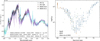 |
Fig. 1 Left: three best-fitting spectra to HD 112863 B, when compared to the spectra of M, L, and T dwarfs included in the SpeX, IRTF, and Allers & Liu (2013) spectral libraries. Right: values of Gk from fitting each of the spectra of the M, L, and T dwarfs in the SpeX, IRTF, and Allers & Liu (2013) spectral libraries to HD 112863 B. |
4.2 Atmospheric model fits
To constrain the physical characteristics of HD 112863 B and HD 206505 B, we fit grids of atmospheric model spectra to the SPHERE spectra of each object. We used the BT-Settl (Allard et al. 2011, 2012) and the Sonora Diamondback (Morley et al. 2024) atmospheric model grids, given their suitability for our targets. In particular, we chose these models since they are applicable to both BDs and VLMSs; given that our objects are early to mid-L dwarfs (see Sect. 4.1) and have M near the HBMM (see Appendix F), both objects could be either a BD or a VLMS, so any model grid used must accommodate both possibilities. Additionally, we chose these grids because they include some form of cloud treatment, since cloud formation is relevant both for BDs (Ackerman & Marley 2001; Helling et al. 2008; Stephens et al. 2009) and for UCDs as a whole (Marley et al. 2002; Cushing et al. 2006, 2008; Saumon & Marley 2008).
The BT-Settl atmospheric model grid was one of the first sets of simulated spectra to be able to match the L-T transition. The BT-Settl grid is also able to match the M dwarf population in Teff vs color space more accurately compared to previous model grids (Allard et al. 2012). The Sonora Diamondback atmospheric model grid consists of spectra that act as boundary conditions for new evolutionary models, that are calculated for objects ranging from 0.5 MJup to 84 MJup. Both metallicity, [M/H], and sedimentation efficiency, fsed, (inversely corresponding to cloud thickness) are included as varied parameters within the Sonora Diamondback atmospheric model grid, which is distinct compared to older and more simplistic grids where Teff and log g are typically the only available “free” parameters (Morley et al. 2024).
We fit the atmospheric models to each object using species. species uses a given atmospheric model grid to fit physical parameters to an observed spectrum by linearly interpolating between the synthetic spectra within the grid, and extrapolating from the interpolated spectrum to obtain the corresponding parameter values. To probe the posterior distribution of each physical parameter, we used nested sampling with species via the Ultranest Python package (Buchner 2016, 2019, 2021); nested sampling is better at probing multi-model distributions, that occur when fitting atmospheric model grids, compared to Markov chain Monte Carlo (MCMC) algorithms (e.g., Hurt et al. 2024). We sampled the posterior distributions of each model grid’s parameters using 500 live points. Using gaussian kernel density estimation, we computed the highest posterior density interval for each parameter, in order to properly estimate the median and 1σ intervals for any posteriors that may be multi-modal. For any fits with multi-modal posteriors, we compared the samples from a single mode of one parameter with the those of all other multi-modal parameters, to correctly match the corresponding modes between all parameters.
When fitting each of the atmospheric model grids, we included a Gaussian prior on the M of HD 112863 B and HD 206505 B, using their dynamical masses from the updated orbit fits (M = ![Mathematical equation: $\[77.7_{-3.3}^{+3.4}\]$](/articles/aa/full_html/2025/09/aa55310-25/aa55310-25-eq10.png) MJup and M = 79.8 ± 1.8 MJup, respectively, see Appendix F). We also included a Gaussian prior on the ϖ of each target (ϖ = 26.96 ± 0.03 mas and ϖ = 22.77 ± 0.02 mas, respectively, Rickman et al. 2024). We set a uniform prior on the effective temperature Teff with lower and upper bounds of 1300 K to 2500 K, based on previous observational studies of early to mid-L dwarfs (Kirkpatrick 2005; Rajpurohit et al. 2012; Gizis et al. 2013; Dieterich et al. 2014; Lodieu et al. 2014; Filippazzo et al. 2015; Dupuy & Liu 2017; Hurt et al. 2024; Li et al. 2024). species uses the log g and R value at each step to calculate the corresponding M, and thereby ensures that the prior on M is respected when computing the log-likelihood. L is a derived parameter calculated using the posteriors of Teff and R.
MJup and M = 79.8 ± 1.8 MJup, respectively, see Appendix F). We also included a Gaussian prior on the ϖ of each target (ϖ = 26.96 ± 0.03 mas and ϖ = 22.77 ± 0.02 mas, respectively, Rickman et al. 2024). We set a uniform prior on the effective temperature Teff with lower and upper bounds of 1300 K to 2500 K, based on previous observational studies of early to mid-L dwarfs (Kirkpatrick 2005; Rajpurohit et al. 2012; Gizis et al. 2013; Dieterich et al. 2014; Lodieu et al. 2014; Filippazzo et al. 2015; Dupuy & Liu 2017; Hurt et al. 2024; Li et al. 2024). species uses the log g and R value at each step to calculate the corresponding M, and thereby ensures that the prior on M is respected when computing the log-likelihood. L is a derived parameter calculated using the posteriors of Teff and R.
As done for the empirical spectra fitting (see Sect. 4.1), we did not include any parameters to account for any potential RV shift, AV, or visual reddening, RV, when computing the atmospheric model fits. Moreover, we did not include any parameters in our fits to account for rotational broadening, since the resolution of our observed spectra are too low to detect this phenomenon. We also chose to apply weights to each observed spectrophotometric point when calculating the log-likelihood, following the same approach as described in Sect. 4.1: photometric points are weighted based on the FWHM of the associated filter, while spectroscopic points are weighted based on the spacing between wavelengths.
The atmospheric model fit results for HD 112863 B are shown in Fig. 3 using the BT-Settl grid and in Fig. 4 using the Sonora Diamondback grid. The parameter values from both of these fits, along with the evidence of each model, Z, are compared in Table 1. The BT-Settl fit is strongly bimodal (see Figs. 3 and G.1), although the first mode (corresponding to Teff = ![Mathematical equation: $\[1757_{-36}^{+37}\]$](/articles/aa/full_html/2025/09/aa55310-25/aa55310-25-eq25.png) K, log g =
K, log g = ![Mathematical equation: $\[4.973_{-0.063}^{+0.057}\]$](/articles/aa/full_html/2025/09/aa55310-25/aa55310-25-eq26.png) ) is approximately three Article number, page 8 of 21 times higher in probability for Teff compared to the second mode (corresponding to Teff =
) is approximately three Article number, page 8 of 21 times higher in probability for Teff compared to the second mode (corresponding to Teff = ![Mathematical equation: $\[2002_{-24}^{+23}\]$](/articles/aa/full_html/2025/09/aa55310-25/aa55310-25-eq27.png) K, log g =
K, log g = ![Mathematical equation: $\[5.253_{-0.033}^{+0.037}\]$](/articles/aa/full_html/2025/09/aa55310-25/aa55310-25-eq28.png) ), indicating that the first mode is somewhat preferred. One possible source of this bimodality is an exchange between fitting to the peak at 1.4 μm and fitting to the shape of the spectra from 1.2–1.3 μm. Fig. 1 of Hurt et al. (2024) shows that BT-Settl models of higher Teff, and somewhat similarly, those of higher log g, have higher flux at 1.4 μm, that better matches the peak at 1.4 μm in the spectra of HD 112863 B. Meanwhile, BT-Settl models of lower Teff show a lower flux around 1.2–1.3 μm compared to those of higher Teff, better matching the spectra of HD 112863 B at 1.2–1.3 μm.
), indicating that the first mode is somewhat preferred. One possible source of this bimodality is an exchange between fitting to the peak at 1.4 μm and fitting to the shape of the spectra from 1.2–1.3 μm. Fig. 1 of Hurt et al. (2024) shows that BT-Settl models of higher Teff, and somewhat similarly, those of higher log g, have higher flux at 1.4 μm, that better matches the peak at 1.4 μm in the spectra of HD 112863 B. Meanwhile, BT-Settl models of lower Teff show a lower flux around 1.2–1.3 μm compared to those of higher Teff, better matching the spectra of HD 112863 B at 1.2–1.3 μm.
The results from both fits indicate that the Teff of HD 112863 B corresponds to an early to mid-L spectral type (Dieterich et al. 2014; Filippazzo et al. 2015), which supports the conclusions made in Sect. 4.1. The results from both fits also indicate that HD 112863 B has a high log g (approximately 5 dex, Chabrier & Baraffe 2000), a characteristic of older UCDs (Martin et al. 2017), that coincides with the suspected older age (greater than 1 Gyr) of the HD 112863 system (Rickman et al. 2024). The results from the Sonora Diamondback fit indicate that HD 112863 B has thick cloud cover (since fsed < 2, Morley et al. 2024), as well as a near-solar [M/H] (see Fig. G.2).
The atmospheric model fit results for HD 206505 B are shown in Fig. 5 using the BT-Settl grid and in Fig. 6 using the Sonora Diamondback grid. The parameter values from both of these fits, along with the Z of each model, are compared in Table 2. Both fits for HD 206505 B indicate Teff values approximately corresponding to an early to mid-L type (Dieterich et al. 2014; Filippazzo et al. 2015), again supporting the conclusions from Sect. 4.1. The log g values from both fits are also high, therefore coinciding with the suspected older age of HD 206505 B (Rickman et al. 2024). Finally, the Sonora Diamondback fit shows that HD 206505 B has thick cloud cover and that [M/H] is near-solar.
For both HD 112863 B and HD 206505 B, BT-Settl is the favored model grid over Sonora Diamondback, since the Bayes factor is >100 between the two models for both objects, respectively (see Tables 1 and 2). We note that the [M/H] found for both HD 112863 B and HD 206505 B from the Sonora Diamondback fits (see Table 1 and Table 2) are consistent with [Fe/H] found for the host stars in Rickman et al. (2024).
While R measurements from transits of UCDs with measured masses near the HBMM find 0.8 RJup ≲ R ≲ 1.5 RJup (Pont et al. 2006; Cañas et al. 2018; Acton et al. 2020; Grieves et al. 2021; Cañas et al. 2022; Sebastian et al. 2022; Lambert et al. 2023; Ferreira dos Santos et al. 2024), the results from nearly all of our atmospheric model fits yield R near or above the upper bound of this range, with the only exception being the first mode of the BT-Settl fit to HD 112863 B. Discrepancies regarding R computed from atmospheric modeling are a known issue (e.g., Zalesky et al. 2019; Lueber et al. 2022; Hood et al. 2023; Zhang et al. 2023; Tobin et al. 2024), although this usually involves an underestimation of R by the models, not an overestimation. One potential explanation for this may lie in the estimate of log g found by our model fits; log g for older (greater than 1 Gyr) UCDs specifically near the HBL are expected to be approximately 5.5 dex (von Boetticher et al. 2019), higher than our estimates, which would correspond to a lower R. Another possible explanation for the unphysically large R in our atmospheric model fits is that HD 112863 B and/or HD 206505 B binaries. However, we note that neither HD 206505 B nor HD 112863 B demonstrate signs of binarity in their PSF shapes in the SPHERE data; from the SPHERE images, binarity is ruled out for both companions down to approximately 2 AU.
Hurt et al. (2024) found that proper treatment for modeling dust grains in the atmospheres of UCDs may explain model discrepancies, including at 1.4 μm, where our residuals are typically largest (~5σ, see Figs. 3, 4, 5, and 6). Hurt et al. (2024) also found that dust grains may also explain the lower-than-expected log g values, and conversely the higher-than-expected R values, found in some UCD atmospheric model fits. Additionally, the large residuals around 1.4 μm in our model fits may be the result of an imperfect telluric correction, that can occur during observations with variable atmospheric conditions where simultaneous monitoring of the host star’s flux is not available, as described in Brown-Sevilla et al. (2023). However, the shape of the spectra of HD 112863 B and HD 206505 B, including around 1.4 μm, match that of other objects, per our comparisons with empirical spectra (see Sect. 4.1). This implies that the large residuals in our atmospheric model fits are not due to any issues unique to our observations or objects’ spectra, but instead may be the result of limitations in the models. Although one such limitation may be incomplete water vapor opacity line lists included in the models, particularly in the older BT-Settl grids, this is unlikely to explain the large residuals seen at 1.4 μm. Both sets of models fail to fit this region of the spectra, including Sonora Diamondback, which includes the latest water line lists. Overall, a thorough investigation of the tendency towards unphysically large R in our model fits is beyond the scope of this work.
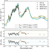 |
Fig. 3 Median atmospheric model of the first mode (demarcated olive line) and the median atmospheric model of the second mode (demarcated cyan line) from the BT-Settl grid fit to the SPHERE photometry and spectroscopy of HD 112863 B (see Fig. G.1). Included are 25 models chosen randomly from the first mode (translucent olive lines) and 25 models chosen randomly from the second mode (translucent cyan lines) of the posterior distribution. The residuals between the SPHERE data and both the first mode (ΔFλ(σ)1) as well as the second mode (ΔFλ(σ)2) are shown. |
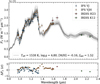 |
Fig. 4 Median atmospheric model (black line, see Fig. G.2) from the Sonora Diamondback grid fit to the SPHERE photometry and spectroscopy of HD 112863 B, along with 50 models chosen randomly from the posterior distribution (gray lines). |
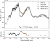 |
Fig. 5 Median atmospheric model (black line, see Fig. G.3) from the BT-Settl grid fit to the SPHERE photometry and spectroscopy of HD 206505 B, along with 50 models chosen randomly from the posterior distribution (gray lines). |
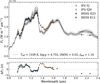 |
Fig. 6 Median atmospheric model (black line, see Fig. G.4) from the Sonora Diamondback grid fit to the SPHERE photometry and spectroscopy of HD 206505 B, along with 50 models chosen randomly from the posterior distribution (gray lines). |
5 Evolutionary model tracks
To investigate whether HD 112863 B and HD 206505 B are stellar or substellar, and how they compare to evolutionary tracks, we compared the atmospheric-model-derived L of both companions with L versus age evolutionary models of UCDs. We chose to use the Sonora Diamondback evolutionary models for this purpose, since they include the evolution of both VLMSs and BDs with a range of characteristics. More specifically, the Sonora Diamondback evolutionary models include tracks without clouds, clouds dependent on Teff (hybrid), and clouds dependent on Teff and log g (hybrid-grav), as well as subsolar (−0.5), solar (0.0), and supersolar (+0.5) [M/H] (Morley et al. 2024).
Because clouds are relevant for modeling L dwarfs (see Sects. 1 and 4.2), we chose to use only the two sets of Sonora Diamondback tracks that include clouds, which are the hybrid and hybrid-grav models. We used the corresponding system ages listed in Rickman et al. (2024) as the age of each companion (3.31 ± 2.91 Gyr for HD 112863 B and 3.94 ± 2.51 Gyr for HD 206505 B).
The comparison of HD 112863 B and HD 206505 B with the Sonora Diamondback L evolutionary tracks are shown in Figs. 7 and 8. We find that the dynamical mass, measured L, and system ages are consistent with the evolutionary tracks for both objects for the hybrid cases (see Figs. 7a and 8a, respectively). From these comparisons, we also conclude that both HD 112863 B and HD 206505 B are likely VLMSs, given that L in all of the tracks for both companions only correspond to objects that either have already reached a stable L thanks to H burning, or will do so at some point as they age.
While the evolutionary model tracks are consistent with the companion L and ages in the hybrid scenario, there is a discrepancy between the companion L and ages in the hybridgrav scenarios (see Figs. 7b and 8b), with the most tension occurring between hybrid-grav tracks and the HD 206505 B BT-Settl L. This is because the hybrid-grav tracks predict a lower L than the hybrid tracks after approximately 1 Gyr. We note that this difference in L beyond 1 Gyr between the hybrid and hybridgrav tracks is expected, since Morley et al. (2024) shows that hybrid-grav models are ≈ 100 K cooler in Teff beyond 1 Gyr for objects M ~ 80 MJup compared to hybrid models.
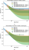 |
Fig. 7 System age and L of HD 112863 B compared to the Sonora Diamondback hybrid (a) and hybrid-grav (b) evolutionary models (Morley et al. 2024). The L values of both the first mode (olive circle) and the second mode (cyan circle) from the BT-Settl atmospheric model fit to HD 112863 B are included (see Fig. G.1). The shaded regions show the model L predictions that correspond to the 1σ dynamical mass constraint of HD 112863 B ( |
![Mathematical equation: $\[77.7_{-3.3}^{+3.4}\]$](/articles/aa/full_html/2025/09/aa55310-25/aa55310-25-eq39.png)
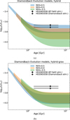 |
Fig. 8 Same as Fig. 7 but for HD 206505 B. The shaded regions show the model L predictions that correspond to the 1σ dynamical mass constraint of HD 206505 B (79.8 ± 1.8 MJup, see Appendix F). |
6 Conclusions
We report the spectral analysis of two benchmark L dwarfs orbiting HD 112863 and HD 206505. We report the following results:
HD 112863 B is spectral type L3 ±1 while HD 206505 B is spectral type L2 ±1, confirming the conclusions from Rickman et al. (2024);
for HD 112863 B, Teff =
![Mathematical equation: $\[1757_{-36}^{+37}\]$](/articles/aa/full_html/2025/09/aa55310-25/aa55310-25-eq40.png) K or
K or ![Mathematical equation: $\[2002_{-24}^{+23}\]$](/articles/aa/full_html/2025/09/aa55310-25/aa55310-25-eq41.png) K, log g =
K, log g = ![Mathematical equation: $\[4.973_{-0.063}^{+0.057}\]$](/articles/aa/full_html/2025/09/aa55310-25/aa55310-25-eq42.png) or
or ![Mathematical equation: $\[5.253_{-0.033}^{+0.037}\]$](/articles/aa/full_html/2025/09/aa55310-25/aa55310-25-eq43.png) , R =
, R = ![Mathematical equation: $\[1.428_{-0.078}^{+0.082}\]$](/articles/aa/full_html/2025/09/aa55310-25/aa55310-25-eq44.png) RJup or
RJup or ![Mathematical equation: $\[1.039_{-0.059}^{+0.041}\]$](/articles/aa/full_html/2025/09/aa55310-25/aa55310-25-eq45.png) RJup, and log L/L⊙ =
RJup, and log L/L⊙ = ![Mathematical equation: $\[-3.733_{-0.027}^{+0.023}\]$](/articles/aa/full_html/2025/09/aa55310-25/aa55310-25-eq46.png) or
or ![Mathematical equation: $\[-3.790_{-0.020}^{+0.020}\]$](/articles/aa/full_html/2025/09/aa55310-25/aa55310-25-eq47.png) ;
;for HD 206505 B, Teff =
![Mathematical equation: $\[1754_{-13}^{+13}\]$](/articles/aa/full_html/2025/09/aa55310-25/aa55310-25-eq48.png) K, log g =
K, log g = ![Mathematical equation: $\[4.919_{-0.029}^{+0.031}\]$](/articles/aa/full_html/2025/09/aa55310-25/aa55310-25-eq49.png) , R =
, R = ![Mathematical equation: $\[1.543_{-0.053}^{+0.057}\]$](/articles/aa/full_html/2025/09/aa55310-25/aa55310-25-eq50.png) RJup, and log L/L⊙ =
RJup, and log L/L⊙ = ![Mathematical equation: $\[-3.669_{-0.021}^{+0.019}\]$](/articles/aa/full_html/2025/09/aa55310-25/aa55310-25-eq51.png) ;
;the R found for both HD 112863 B and HD 206505 B in the majority of our atmospheric model fits are unphysically large, although this may be due to limitations with the atmospheric models themselves;
the measured L, dynamical masses, and system ages of HD 112863 B and HD 206505 B are in agreement with the predictions from evolutionary models;
both HD 112863 B and HD 206505 B are likely VLMSs.
The most significant difference in results compared to Rickman et al. (2024) is the photometry of each companion, as shown in Table D.1 (versus Table 2 of Rickman et al. 2024). The biggest impact of this change is the CMD, where the placement of each companion, especially HD 112863 B, is more accurate (see Fig. E.1). Regardless, the overall spectral classification of HD 112863 B and HD 206505 B remain in agreement with this work.
We note that the constraints on the spectral and physical parameters of HD 206505 B are more precise than that of HD 112863 B (see Fig. 2 versus Fig. 1, Table 2 versus Table 1, and Table F.1), a result of HD 112863 B being detected at a S/N approximately ten times lower than HD 206505 B (see Sect. 3.2). This is explained by the attenuation of HD 112863 B’s flux by the coronagraph, in combination with the fact that HD 112863 B lies at a closer ρ than HD 206505 B, in a region of higher noise.
HD 112863 B is one of a few companions successfully detected in HCI despite being within the IWA of an instrument’s coronagraph (e.g., Franson et al. 2024). Such detections aid in understanding the feasibility of observing companions in HCI at ρ previously viewed as inaccessible by current instruments.
The system ages are the limiting factor in determining where HD 112863 B and HD 206505 B are in their thermal evolution (as seen in Figs. 7 and 8). Future work on the HD 112863 and HD 206505 systems could therefore involve deriving stronger constraints on the system ages through asteroseismology (e.g., Huber et al. 2009; Chaplin et al. 2011). Currently planned future work on these systems including further spectral analysis of both companions using data from VLTI/GRAVITY and VLT/HiRISE (Rickman et al., in prep.), that will provide constraints on the C/O ratio of the companions (GRAVITY Collaboration 2017), and enable the detection of rotational broadening in their spectra (Vigan et al. 2024). Finally, the additional spectra of HD 112863 B and HD 206505 B from these two sets of observations will provide verification of our conclusions presented here, including the tentative classification of both companions as VLMSs.
HD 112863 B and HD 206505 B add to the growing list of UCD and exoplanet companions detected in HCI with dynamical mass measurements. Similar companions included in this list are HD 72946 B (M = 69.5 ± 0.5 MJup, Balmer et al. 2023), HD 4747 B (M = ![Mathematical equation: $\[65.3_{-3.3}^{+4.4}\]$](/articles/aa/full_html/2025/09/aa55310-25/aa55310-25-eq52.png) MJup, Crepp et al. 2018), HR 7672 B (M = 72.7 ± 0.8 MJup, Brandt et al. 2019), and HD 984 B (M = 61 ± 4 MJup, Franson et al. 2022). Each of these substellar companions are near the HBL and have Teff ≥ 1500 K and log g ≥ 5, with HD 72946 B, HD 4747 B, and HR 7672 B specifically having ages greater than 1 Gyr (Balmer et al. 2023; Crepp et al. 2018; Meshkat et al. 2015; Wang et al. 2022). Building a larger sample of such objects is valuable since they can be used collectively to empirically constrain mass-dependent boundaries such as the HBL (e.g., Dupuy & Liu 2017) as well as to more robustly test atmospheric and evolutionary models (e.g., Grieves et al. 2021; Iyer et al. 2023). In particular, our work shows that current atmospheric models may be limited in explaining the full shape of spectra of older UCDs near the HBL and in estimating their R. Additional detections are needed to determine if these discrepancies are a true shortcoming of the models or only unique to these two objects.
MJup, Crepp et al. 2018), HR 7672 B (M = 72.7 ± 0.8 MJup, Brandt et al. 2019), and HD 984 B (M = 61 ± 4 MJup, Franson et al. 2022). Each of these substellar companions are near the HBL and have Teff ≥ 1500 K and log g ≥ 5, with HD 72946 B, HD 4747 B, and HR 7672 B specifically having ages greater than 1 Gyr (Balmer et al. 2023; Crepp et al. 2018; Meshkat et al. 2015; Wang et al. 2022). Building a larger sample of such objects is valuable since they can be used collectively to empirically constrain mass-dependent boundaries such as the HBL (e.g., Dupuy & Liu 2017) as well as to more robustly test atmospheric and evolutionary models (e.g., Grieves et al. 2021; Iyer et al. 2023). In particular, our work shows that current atmospheric models may be limited in explaining the full shape of spectra of older UCDs near the HBL and in estimating their R. Additional detections are needed to determine if these discrepancies are a true shortcoming of the models or only unique to these two objects.
Data availability
The S/N maps from each SPHERE dataset (all IRDIS and IFS photometry/spectroscopy), the final spectra of both companions as extracted from these datasets, and the posterior distributions of all the parameters obtained from the nested sampling atmospheric model fits to each companion’s spectra are available on the DACE platform https://doi.org/10.82180/dace-mf2z5vn5.
Acknowledgements
We thank João Faria for his guidance regarding proper estimation of credible intervals for multi-modal posterior distributions. We thank Matthias Samland for his insightful discussions that led to including weather-driven frame selection as a component of our data reduction procedure. This work has been carried out within the framework of the National Centre of Competence in Research PlanetS supported by the Swiss National Science Foundation under grants 51NF40_182901 and 51NF40_205606. The authors acknowledge the financial support of the SNSF. This publications makes use of the Data and Analysis Center for Exoplanets (DACE), which is a facility based at the University of Geneva (CH) dedicated to extrasolar planets data visualization, exchange and analysis. DACE is a platform of the Swiss National Centre of Competence in Research (NCCR) PlanetS, federating the Swiss expertise in Exoplanet research. The DACE platform is available at https://dace.unige.ch. This work has made use of data from the European Space Agency (ESA) mission Gaia (https://www.cosmos.esa.int/gaia), processed by the Gaia Data Processing and Analysis Consortium (DPAC, https://www.cosmos.esa.int/web/gaia/dpac/consortium). Funding for the DPAC has been provided by national institutions, in particular the institutions participating in the Gaia Multilateral Agreement. This research made use of the SIMBAD database and the VizieR Catalog access tool, both operated at the CDS, Strasbourg, France. The original descriptions of the SIMBAD and VizieR services were published in Wenger et al. (2000) and Ochsenbein et al. (2000). This research has made use of NASA’s Astrophysics Data System Bibliographic Services.
Appendix A Uncorrected and corrected spectra
Shown here are the status of the spectra of HD 112863 B and HD 206505 B at each step of the data reduction process, as detailed in Sect. 3. The spectra of both companions required correction for the weather during observations (see Sect. 3.2.1 and Appendix B), the results of which are shown in Fig. A.1b and Fig. A.2b. Additionally, the spectrum of HD 112863 B required correction for the transmittance of the SPHERE coronagraph (see Sect. 3.2.2 and Appendix C), the result of which is shown in Fig. A.1c.
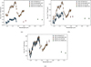 |
Fig. A.1 (a) Original flux spectra of HD 112863 B before accounting for the effects of weather and the coronagraphic attenuation of the companion. (b) Partially corrected flux spectra of HD 112863 B after accounting for weather effects (see Sect. 2 and Sect. 3.2.1). (c) Final flux spectra of HD 112863 B, after accounting for both the effects of weather and the coronagraphic attenuation of the companion (see Sect. 3.2.2). |
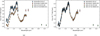 |
Fig. A.2 Flux spectra of HD 206505 B, before (a) and after (b) accounting for the effects of weather on the datasets (see Sect. 2 and Sect. 3.2.1). |
Appendix B DTTS data
Included here are the flux measurements recorded by the SPARTA computer on the DTTS of SPHERE, for both epochs of HD 112863 and HD 206505 observations. The DTTS flux measurements for the two epochs of HD 112863 observations are shown in Fig. B.1 and Fig. B.2, while the DTTS flux measurements for the two epochs of HD 206505 observations are shown in Fig. B.3 and Fig. B.4. The durations of the science and flux cubes are also shown for each set of observations.
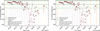 |
Fig. B.1 DTTS flux measurements of HD 112863 during the 2021-04-07 IRDIS H23 (left) and IFS YJ (right) observations. Green lines indicate the median and ±1 MAD of the measurements, that are the criteria used when excluding science frames based on weather conditions (see Sect. 3.2.1). |
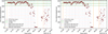 |
Fig. B.2 Same as Fig. B.1 but for HD 112863 during the 2022-01-30 IRDIS K12 (left) and IFS YJH (right) observations. |
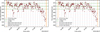 |
Fig. B.3 Same as Fig. B.1 but for HD 206505 during the 2019-01-31 IRDIS H23 (left) and IFS YJ (right) observations. |
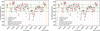 |
Fig. B.4 Same as Fig. B.1 but for HD 206505 during the 2021-07-01 IRDIS K12 (left) and IFS YJH (right) observations. |
Appendix C Coronagraph transmission profiles
Included here are the on-sky-measured transmission profiles of the N_ALC_YJH_S coronagraph integrated in SPHERE. The measured transmission values, along with the interpolated profiles, are shown in Fig. C.1 for IRDIS H23 and K12 and in Fig. C.2 for IFS YJ. Because transmission measurements of the coronagraph over the IFS YJH wavelength range are not available, we interpolated between the measured transmission values for IRDIS H23 and IFS YJ to generate coronagraph transmission profiles for IFS YJH, shown in Fig. C.3.
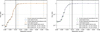 |
Fig. C.1 Coronagraph transmission profiles for IRDIS H23 (left) and K12 (right). Shown here are the measured values taken on-sky with seeing conditions of ~0.8 arcsec (A. Vigan), as well as the cubic spline interpolation to these values. These interpolations were treated as radial profiles to create coronagraphic transmission images, in order to directly correct the HD 112863 science frames (see Sect. 3.2.2). Also shown are the equivalent ρ at 10 pixels, 20 pixels, 30 pixels, accounting for the difference in pixel scale between each band. |
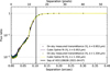 |
Fig. C.2 Same as Fig. C.1 but for the coronagraph transmission profiles for IFS YJ. The measurements and interpolations for the first and last wavelength of IFS YJ are highlighted. |
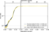 |
Fig. C.3 Coronagraph transmission profiles for IFS YJH. Shown here are the results of the bivariate spline interpolation to the IFS YJ and IRDIS H23 measured values, at each of the IFS YJH wavelengths. The interpolations for the first and last wavelength of IFS YJH are highlighted. The interpolations were treated as radial profiles to create coronagraphic transmission images, in order to directly correct the HD 112863 science frames (see Sect. 3.2.2). |
Appendix D Updated relative astrometry and photometry
We recomputed the relative astrometry and photometry of HD 112863 B and HD 206505 B, with the results shown in Table D.1; the data reduction approach used in Rickman et al. (2024) did not include some of the steps described in Sect. 3.2.1 and Sect. 3.2.2, resulting in a flux offset between the two epochs of spectrophotometric observations for both companions (see Appendix A). We note that the updated relative astrometry is consistent with the values presented in Rickman et al. (2024) within ±1σ.
Updated relative astrometry and photometry of HD 112863 B and HD 206505 B.
Appendix E Updated color-magnitude diagram
Since the data reduction approach used in Rickman et al. (2024) did not include some of the steps described in Sect. 3.2.1 and Sect. 3.2.2, we generated a new CMD, shown in Fig. E.1, that uses the updated photometry of HD 112863 B and HD 206505 B from this work (see Appendix D, specifically Table D.1).
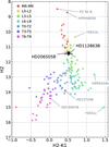 |
Fig. E.1 Updated CMD (compared to Fig. 4 of Rickman et al. 2024) showing HD 112863 B and HD 206505 B (black squares, from Table D.1) in comparison to the population of field brown dwarfs (circle symbols), as well as some notable substellar companions (star symbols). Field brown dwarfs are color-coded by spectral classification. |
Appendix F Updated orbit fits
Using the updated relative astrometry shown in Table D.1, we obtain new orbit fits of both systems using the orbit-fitting code orvara (Brandt et al. 2021). We use the RV measurements, along with the HIPPARCOS-Gaia catalog of accelerations (HGCA, Brandt 2021) as outlined in Rickman et al. (2022) and Rickman et al. (2024), and incorporate the updated astrometry as presented in this paper.
For both systems, we performed an orbit fit using a parallel-tempered MCMC with 15 temperatures. For each temperature, we used 100 walkers with 40000 steps per walker thinned by a factor of 50. We used a log-flat prior on the host star mass in order to derive the mass of the star dynamically. The resulting updated dynamical masses and orbital parameters are all in agreement with Rickman et al. (2024), and are shown in Table F.1. The dynamical mass of HD 206505 B did not change from Rickman et al. (2024), and the dynamical mass of HD 112863 B changed fractionally with the previous value of ![Mathematical equation: $\[77.1_{-2.8}^{+2.9}\]$](/articles/aa/full_html/2025/09/aa55310-25/aa55310-25-eq53.png) MJup to now
MJup to now ![Mathematical equation: $\[77.7_{-3.3}^{+3.4}\]$](/articles/aa/full_html/2025/09/aa55310-25/aa55310-25-eq54.png) MJup, which is due to HD 112863 B being within the IWA of the coronagraph and applying the coronagraphic transmission factor as described in Sect. 3.2.2. Despite a slight increase in the uncertainty folded in due to this transmission correction, the orbital parameters are well-defined due to the extensive orbital phase coverage of the RVs (Rickman et al. 2024), and are all in agreement with the previously derived values.
MJup, which is due to HD 112863 B being within the IWA of the coronagraph and applying the coronagraphic transmission factor as described in Sect. 3.2.2. Despite a slight increase in the uncertainty folded in due to this transmission correction, the orbital parameters are well-defined due to the extensive orbital phase coverage of the RVs (Rickman et al. 2024), and are all in agreement with the previously derived values.
Markov chain Monte Carlo orbital posteriors for the orbital fits of each system using orvara (Brandt et al. 2021).
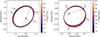 |
Fig. F.1 Updated versions of the top right panels of Fig. 2 and Fig. 3 from Rickman et al. (2024); the measured astrometric positions (blue data points) and orbits of HD 112863 B (left) and HD 206505 B (right) relative to their host stars. The corresponding masses from the orbit fits are represented by the color bar to the right of each plot. |
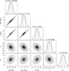 |
Fig. F.2 Corner plot of orbital parameters of HD 112863 B (updated version of Fig. B.1 in Rickman et al. 2024). |
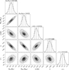 |
Fig. F.3 Corner plot of orbital parameters of HD 206505 B (updated version of Fig. B.2 in Rickman et al. 2024). |
Appendix G Atmospheric parameters posterior distributions
Shown here are the posterior distributions of the parameters from the atmospheric model fits to HD 112863 B and HD 206505 B, using both the BT-Settl and Sonora Diamondback model grids (see Sect. 4.2).
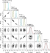 |
Fig. G.1 Posterior distributions of the physical and derived parameters from the BT-Settl atmospheric model fit to HD 112863 B (see Fig. 3). Included are the median values and 1σ credible intervals for both the first mode (dashed olive lines) and the second mode (dashed cyan lines) of the bimodal posteriors. The priors used for ϖ and M are also included (red dotted lines). |
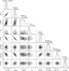 |
Fig. G.2 Posterior distributions of the physical and derived parameters from the Sonora Diamondback atmospheric model fit to HD 112863 B (see Fig. 4). |
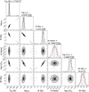 |
Fig. G.3 Posterior distributions of the physical and derived parameters from the BT-Settl atmospheric model fit to HD 206505 B (see Fig. 5). |
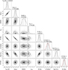 |
Fig. G.4 Posterior distributions of the physical and derived parameters from the Sonora Diamondback atmospheric model fit to HD 206505 B (see Fig. 6). |
References
- Ackerman, A. S., & Marley, M. S. 2001, ApJ, 556, 872 [Google Scholar]
- Acton, J. S., Goad, M. R., Casewell, S. L., et al. 2020, MNRAS, 498, 3115 [NASA ADS] [CrossRef] [Google Scholar]
- Allard, F., Homeier, D., & Freytag, B. 2011, in Astronomical Society of the Pacific Conference Series, 448, 16th Cambridge Workshop on Cool Stars, Stellar Systems, and the Sun, eds. C. Johns-Krull, M. K. Browning, & A. A. West, 91 [Google Scholar]
- Allard, F., Homeier, D., & Freytag, B. 2012, Philos. Trans. Roy. Soc. Lond. A, 370, 2765 [NASA ADS] [Google Scholar]
- Allers, K. N., & Liu, M. C. 2013, ApJ, 772, 79 [NASA ADS] [CrossRef] [Google Scholar]
- Antichi, J., Dohlen, K., Gratton, R. G., et al. 2009, ApJ, 695, 1042 [Google Scholar]
- Balmer, W. O., Pueyo, L., Stolker, T., et al. 2023, ApJ, 956, 99 [NASA ADS] [CrossRef] [Google Scholar]
- Baraffe, I., Chabrier, G., Barman, T. S., Allard, F., & Hauschildt, P. H. 2003, A&A, 402, 701 [NASA ADS] [CrossRef] [EDP Sciences] [Google Scholar]
- Beuzit, J. L., Vigan, A., Mouillet, D., et al. 2019, A&A, 631, A155 [NASA ADS] [CrossRef] [EDP Sciences] [Google Scholar]
- Bouy, H., Brandner, W., Martín, E. L., et al. 2003, AJ, 126, 1526 [CrossRef] [Google Scholar]
- Brandt, T. D. 2021, ApJS, 254, 42 [NASA ADS] [CrossRef] [Google Scholar]
- Brandt, T. D., Dupuy, T. J., & Bowler, B. P. 2019, AJ, 158, 140 [Google Scholar]
- Brandt, T. D., Dupuy, T. J., Bowler, B. P., et al. 2020, AJ, 160, 196 [Google Scholar]
- Brandt, T. D., Dupuy, T. J., Li, Y., et al. 2021, AJ, 162, 186 [NASA ADS] [CrossRef] [Google Scholar]
- Brown-Sevilla, S. B., Maire, A. L., Mollière, P., et al. 2023, A&A, 673, A98 [NASA ADS] [CrossRef] [EDP Sciences] [Google Scholar]
- Buchner, J. 2016, Statist. Comput., 26, 383 [NASA ADS] [CrossRef] [Google Scholar]
- Buchner, J. 2019, PASP, 131, 108005 [Google Scholar]
- Buchner, J. 2021, J. Open Source Softw., 6, 3001 [CrossRef] [Google Scholar]
- Burgasser, A. J. 2014, in Astronomical Society of India Conference Series, 11, Astronomical Society of India Conference Series, 7 [Google Scholar]
- Burgasser, A. J., Kirkpatrick, J. D., Brown, M. E., et al. 2002, ApJ, 564, 421 [NASA ADS] [CrossRef] [Google Scholar]
- Burrows, A., Hubbard, W. B., Lunine, J. I., & Liebert, J. 2001, Rev. Mod. Phys., 73, 719 [Google Scholar]
- Burrows, A., Heng, K., & Nampaisarn, T. 2011, ApJ, 736, 47 [NASA ADS] [CrossRef] [Google Scholar]
- Cañas, C. I., Bender, C. F., Mahadevan, S., et al. 2018, ApJ, 861, L4 [Google Scholar]
- Cañas, C. I., Mahadevan, S., Bender, C. F., et al. 2022, AJ, 163, 89 [CrossRef] [Google Scholar]
- Calamari, E., Faherty, J. K., Visscher, C., et al. 2024, ApJ, 963, 67 [NASA ADS] [CrossRef] [Google Scholar]
- Cardelli, J. A., Clayton, G. C., & Mathis, J. S. 1989, ApJ, 345, 245 [Google Scholar]
- Chabrier, G., & Baraffe, I. 1997, A&A, 327, 1039 [NASA ADS] [Google Scholar]
- Chabrier, G., & Baraffe, I. 2000, ARA&A, 38, 337 [Google Scholar]
- Chabrier, G., Baraffe, I., Allard, F., & Hauschildt, P. 2000, ApJ, 542, 464 [Google Scholar]
- Chabrier, G., Baraffe, I., Phillips, M., & Debras, F. 2023, A&A, 671, A119 [NASA ADS] [CrossRef] [EDP Sciences] [Google Scholar]
- Chaplin, W. J., Kjeldsen, H., Christensen-Dalsgaard, J., et al. 2011, Science, 332, 213 [Google Scholar]
- Charnay, B., Bézard, B., Baudino, J. L., et al. 2018, ApJ, 854, 172 [Google Scholar]
- Cheetham, A., Ségransan, D., Peretti, S., et al. 2018, A&A, 614, A16 [NASA ADS] [CrossRef] [EDP Sciences] [Google Scholar]
- Claudi, R. U., Turatto, M., Gratton, R. G., et al. 2008, SPIE Conf. Ser., 7014, 70143E [Google Scholar]
- Crepp, J. R., Johnson, J. A., Howard, A. W., et al. 2014, ApJ, 781, 29 [Google Scholar]
- Crepp, J. R., Gonzales, E. J., Bechter, E. B., et al. 2016, ApJ, 831, 136 [NASA ADS] [CrossRef] [Google Scholar]
- Crepp, J. R., Principe, D. A., Wolff, S., et al. 2018, ApJ, 853, 192 [Google Scholar]
- Currie, T., Brandt, T. D., Kuzuhara, M., et al. 2020, ApJ, 904, L25 [Google Scholar]
- Cushing, M. C., Rayner, J. T., & Vacca, W. D. 2005, ApJ, 623, 1115 [Google Scholar]
- Cushing, M. C., Roellig, T. L., Marley, M. S., et al. 2006, ApJ, 648, 614 [Google Scholar]
- Cushing, M. C., Marley, M. S., Saumon, D., et al. 2008, ApJ, 678, 1372 [NASA ADS] [CrossRef] [Google Scholar]
- Cutri, R. M., Skrutskie, M. F., van Dyk, S., et al. 2003, VizieR Online Data Catalog: 2MASS All-Sky Catalog of Point Sources (Cutri+ 2003), VizieR On-line Data Catalog: II/246. Originally published in: University of Massachusetts and Infrared Processing and Analysis Center, (IPAC/California Institute of Technology) [Google Scholar]
- Cutri, R. M., Wright, E. L., Conrow, T., et al. 2021, VizieR Online Data Catalog: AllWISE Data Release (Cutri+ 2013), VizieR On-line Data Catalog: II/328. Originally published in: IPAC/Caltech [Google Scholar]
- de Boer, K., & Seggewiss, W. 2008, Stars and Stellar Evolution [Google Scholar]
- Dieterich, S. B., Henry, T. J., Jao, W.-C., et al. 2014, AJ, 147, 94 [NASA ADS] [CrossRef] [Google Scholar]
- Dohlen, K., Langlois, M., Saisse, M., et al. 2008, Proc. SPIE, 7014, 70143L [Google Scholar]
- Dupuy, T. J., & Liu, M. C. 2017, ApJS, 231, 15 [Google Scholar]
- Fernandes, C. S., Van Grootel, V., Salmon, S. J. A. J., et al. 2019, ApJ, 879, 94 [NASA ADS] [CrossRef] [Google Scholar]
- Ferreira dos Santos, T., Rice, M., Wang, X.-Y., & Wang, S. 2024, AJ, 168, 145 [Google Scholar]
- Filippazzo, J. C., Rice, E. L., Faherty, J., et al. 2015, ApJ, 810, 158 [Google Scholar]
- Franson, K., Balmer, W. O., Bowler, B. P., et al. 2024, ApJ, 974, L11 [NASA ADS] [CrossRef] [Google Scholar]
- Franson, K., Bowler, B. P., Brandt, T. D., et al. 2022, AJ, 163, 50 [NASA ADS] [CrossRef] [Google Scholar]
- Fusco, T., Rousset, G., Sauvage, J. F., et al. 2006, Opt. Express, 14, 7515 [NASA ADS] [CrossRef] [Google Scholar]
- Gaia Collaboration (Vallenari, A., et al.) 2023, A&A, 674, A1 [NASA ADS] [CrossRef] [EDP Sciences] [Google Scholar]
- Gizis, J. E., Burgasser, A. J., Berger, E., et al. 2013, ApJ, 779, 172 [NASA ADS] [CrossRef] [Google Scholar]
- Godoy, N., Choquet, E., Serabyn, E., et al. 2024, A&A, 689, A185 [NASA ADS] [CrossRef] [EDP Sciences] [Google Scholar]
- GRAVITY Collaboration (Abuter, R., et al.) 2017, A&A, 602, A94 [NASA ADS] [CrossRef] [EDP Sciences] [Google Scholar]
- Grieves, N., Bouchy, F., Lendl, M., et al. 2021, A&A, 652, A127 [NASA ADS] [CrossRef] [EDP Sciences] [Google Scholar]
- Hagelberg, J., Ségransan, D., Udry, S., & Wildi, F. 2016, MNRAS, 455, 2178 [NASA ADS] [CrossRef] [Google Scholar]
- Helling, C., Dehn, M., Woitke, P., & Hauschildt, P. H. 2008, ApJ, 675, L105 [NASA ADS] [CrossRef] [Google Scholar]
- Hiranaka, K., Cruz, K. L., Douglas, S. T., Marley, M. S., & Baldassare, V. F. 2016, ApJ, 830, 96 [Google Scholar]
- Høg, E., Fabricius, C., Makarov, V. V., et al. 2000, A&A, 355, L27 [Google Scholar]
- Hood, C. E., Fortney, J. J., Line, M. R., & Faherty, J. K. 2023, ApJ, 953, 170 [NASA ADS] [CrossRef] [Google Scholar]
- Huber, D., Stello, D., Bedding, T. R., et al. 2009, Commun. Asteroseismol., 160, 74 [Google Scholar]
- Hurt, S. A., Liu, M. C., Zhang, Z., et al. 2024, ApJ, 961, 121 [NASA ADS] [CrossRef] [Google Scholar]
- Iyer, A. R., Line, M. R., Muirhead, P. S., Fortney, J. J., & Gharib-Nezhad, E. 2023, ApJ, 944, 41 [NASA ADS] [CrossRef] [Google Scholar]
- Kirkpatrick, J. D. 2005, ARA&A, 43, 195 [NASA ADS] [CrossRef] [Google Scholar]
- Kirkpatrick, J. D., Reid, I. N., Liebert, J., et al. 1999, ApJ, 519, 802 [NASA ADS] [CrossRef] [Google Scholar]
- Lambert, M., Bender, C. F., Kanodia, S., et al. 2023, AJ, 165, 218 [NASA ADS] [CrossRef] [Google Scholar]
- Lane, B. F., Zapatero Osorio, M. R., Britton, M. C., Martín, E. L., & Kulkarni, S. R. 2001, ApJ, 560, 390 [Google Scholar]
- Leggett, S. K., & Tremblin, P. 2025, ApJ, 979, 145 [Google Scholar]
- Lewis, B. L., Li, Y., Gibbs, A., et al. 2024, ApJ, 977, 247 [Google Scholar]
- Li, Y., Brandt, T. D., Franson, K., et al. 2024, MNRAS, 533, 3501 [Google Scholar]
- Liu, M. C., Dupuy, T. J., & Ireland, M. J. 2008, ApJ, 689, 436 [NASA ADS] [CrossRef] [Google Scholar]
- Liu, P., Biller, B. A., Kenworthy, M. A., et al. 2025, A&A, 696, L10 [NASA ADS] [CrossRef] [EDP Sciences] [Google Scholar]
- Lloyd, J. P., & Sivaramakrishnan, A. 2005, ApJ, 621, 1153 [Google Scholar]
- Lodieu, N., Boudreault, S., & Béjar, V. J. S. 2014, MNRAS, 445, 3908 [NASA ADS] [CrossRef] [Google Scholar]
- Lueber, A., Kitzmann, D., Bowler, B. P., Burgasser, A. J., & Heng, K. 2022, ApJ, 930, 136 [NASA ADS] [CrossRef] [Google Scholar]
- Marley, M. S., Seager, S., Saumon, D., et al. 2002, ApJ, 568, 335 [NASA ADS] [CrossRef] [Google Scholar]
- Marley, M. S., Saumon, D., Visscher, C., et al. 2021, ApJ, 920, 85 [NASA ADS] [CrossRef] [Google Scholar]
- Marois, C., Lafrenière, D., Doyon, R., Macintosh, B., & Nadeau, D. 2006, ApJ, 641, 556 [Google Scholar]
- Martin, E. L., Basri, G., Delfosse, X., & Forveille, T. 1997, A&A, 327, L29 [Google Scholar]
- Martin, E. C., Mace, G. N., McLean, I. S., et al. 2017, ApJ, 838, 73 [NASA ADS] [CrossRef] [Google Scholar]
- Meshkat, T., Bonnefoy, M., Mamajek, E. E., et al. 2015, MNRAS, 453, 2378 [NASA ADS] [Google Scholar]
- Morley, C. V., Mukherjee, S., Marley, M. S., et al. 2024, ApJ, 975, 59 [NASA ADS] [CrossRef] [Google Scholar]
- Mukherjee, S., Fortney, J. J., Batalha, N. E., et al. 2022, ApJ, 938, 107 [NASA ADS] [CrossRef] [Google Scholar]
- Ochsenbein, F., Bauer, P., & Marcout, J. 2000, A&AS, 143, 23 [NASA ADS] [CrossRef] [EDP Sciences] [Google Scholar]
- Pavlov, A., Möller-Nilsson, O., Feldt, M., et al. 2008, SPIE Conf. Ser., 7019, 701939 [Google Scholar]
- Petit, C., Sauvage, J. F., Sevin, A., et al. 2012, SPIE Conf. Ser., 8447, 84471Z [NASA ADS] [Google Scholar]
- Petit, C., Sauvage, J. F., Fusco, T., et al. 2014, SPIE Conf. Ser., 9148, 91480O [NASA ADS] [Google Scholar]
- Pont, F., Moutou, C., Bouchy, F., et al. 2006, A&A, 447, 1035 [NASA ADS] [CrossRef] [EDP Sciences] [Google Scholar]
- Queloz, D., Mayor, M., Naef, D., et al. 2000, in From Extrasolar Planets to Cosmology: The VLT Opening Symposium, eds. J. Bergeron, & A. Renzini, 548 [Google Scholar]
- Rajpurohit, A. S., Reylé, C., Schultheis, M., et al. 2012, A&A, 545, A85 [NASA ADS] [CrossRef] [EDP Sciences] [Google Scholar]
- Rickman, E. L., Ceva, W., Matthews, E. C., et al. 2024, A&A, 684, A88 [NASA ADS] [CrossRef] [EDP Sciences] [Google Scholar]
- Rickman, E. L., Matthews, E., Ceva, W., et al. 2022, A&A, 668, A140 [NASA ADS] [CrossRef] [EDP Sciences] [Google Scholar]
- Rickman, E. L., Ségransan, D., Hagelberg, J., et al. 2020, A&A, 635, A203 [NASA ADS] [CrossRef] [EDP Sciences] [Google Scholar]
- Samland, M., Bouwman, J., Hogg, D. W., et al. 2021, A&A, 646, A24 [NASA ADS] [CrossRef] [EDP Sciences] [Google Scholar]
- Saumon, D., & Marley, M. S. 2008, ApJ, 689, 1327 [Google Scholar]
- Sauvage, J.-F., Fusco, T., Petit, C., et al. 2016, J. Astron. Telesc. Instrum. Syst., 2, 025003 [Google Scholar]
- Sebastian, D., Guenther, E. W., Deleuil, M., et al. 2022, MNRAS, 516, 636 [NASA ADS] [CrossRef] [Google Scholar]
- Stephens, D. C., Leggett, S. K., Cushing, M. C., et al. 2009, ApJ, 702, 154 [NASA ADS] [CrossRef] [Google Scholar]
- Stolker, T., Quanz, S. P., Todorov, K. O., et al. 2020, A&A, 635, A182 [EDP Sciences] [Google Scholar]
- Suárez Valles, M., Fedrigo, E., Donaldson, R. H., et al. 2012, SPIE Conf. Ser., 8447, 84472Q [Google Scholar]
- Tobin, T. L., Currie, T., Li, Y., et al. 2024, AJ, 167, 205 [NASA ADS] [CrossRef] [Google Scholar]
- Udry, S., Mayor, M., Queloz, D., Naef, D., & Santos, N. 2000, in From Extrasolar Planets to Cosmology: The VLT Opening Symposium, eds. J. Bergeron, & A. Renzini, 571 [Google Scholar]
- Venner, A., Vanderburg, A., & Pearce, L. A. 2021, AJ, 162, 12 [NASA ADS] [CrossRef] [Google Scholar]
- Vigan, A. 2020, vlt-sphere: Automatic VLT/SPHERE data reduction and analysis, Astrophysics Source Code Library, [record ascl:2009.002] [Google Scholar]
- Vigan, A., Gry, C., Salter, G., et al. 2015, MNRAS, 454, 129 [NASA ADS] [CrossRef] [Google Scholar]
- Vigan, A., El Morsy, M., Lopez, M., et al. 2024, A&A, 682, A16 [NASA ADS] [CrossRef] [EDP Sciences] [Google Scholar]
- von Boetticher, A., Triaud, A. H. M. J., Queloz, D., et al. 2019, A&A, 625, A150 [NASA ADS] [CrossRef] [EDP Sciences] [Google Scholar]
- Wang, J., Kolecki, J. R., Ruffio, J.-B., et al. 2022, AJ, 163, 189 [CrossRef] [Google Scholar]
- Wenger, M., Ochsenbein, F., Egret, D., et al. 2000, A&AS, 143, 9 [NASA ADS] [CrossRef] [EDP Sciences] [Google Scholar]
- Zalesky, J. A., Line, M. R., Schneider, A. C., & Patience, J. 2019, ApJ, 877, 24 [Google Scholar]
- Zhang, Z. H., Homeier, D., Pinfield, D. J., et al. 2017, MNRAS, 468, 261 [NASA ADS] [CrossRef] [Google Scholar]
- Zhang, Z., Mollière, P., Hawkins, K., et al. 2023, AJ, 166, 198 [NASA ADS] [CrossRef] [Google Scholar]
- Zurlo, A., Vigan, A., Mesa, D., et al. 2014, A&A, 572, A85 [NASA ADS] [CrossRef] [EDP Sciences] [Google Scholar]
From the VLT SPHERE User Manual, 18th release.
Paranal Astronomical Site Monitoring (ASM) data for 2021-04-07: https://www.eso.org/asm/ui/publicLog?name=Paranal&startDate=2021-04-07T21:00:00.000Z&hoursInterval=15
Paranal ASM data for 2022-01-30: https://www.eso.org/asm/ui/publicLog?name=Paranal&startDate=2022-01-30T22:00:00.000Z&hoursInterval=15
Paranal ASM data for 2019-08-06: https://www.eso.org/asm/ui/publicLog?name=Paranal&startDate=2019-08-06T21:00:00.000Z&hoursInterval=15
Paranal ASM data for 2021-07-01: https://www.eso.org/asm/ui/publicLog?name=Paranal&startDate=2021-07-01T21:00:00.000Z&hoursInterval=15
The corrections for the ND filter transmission make use of the ND filter curves available at: https://www.eso.org/sci/facilities/paranal/instruments/sphere/inst/filters.html
From the VLT SPHERE User Manual, 18th release.
AV estimates taken from Gaia data release 3 (Gaia Collaboration 2023).
All Tables
Markov chain Monte Carlo orbital posteriors for the orbital fits of each system using orvara (Brandt et al. 2021).
All Figures
|
Fig. 1 Left: three best-fitting spectra to HD 112863 B, when compared to the spectra of M, L, and T dwarfs included in the SpeX, IRTF, and Allers & Liu (2013) spectral libraries. Right: values of Gk from fitting each of the spectra of the M, L, and T dwarfs in the SpeX, IRTF, and Allers & Liu (2013) spectral libraries to HD 112863 B. |
| In the text | |
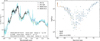 |
Fig. 2 Same as Fig. 1 but for HD 206505 B. |
| In the text | |
|
Fig. 3 Median atmospheric model of the first mode (demarcated olive line) and the median atmospheric model of the second mode (demarcated cyan line) from the BT-Settl grid fit to the SPHERE photometry and spectroscopy of HD 112863 B (see Fig. G.1). Included are 25 models chosen randomly from the first mode (translucent olive lines) and 25 models chosen randomly from the second mode (translucent cyan lines) of the posterior distribution. The residuals between the SPHERE data and both the first mode (ΔFλ(σ)1) as well as the second mode (ΔFλ(σ)2) are shown. |
| In the text | |
|
Fig. 4 Median atmospheric model (black line, see Fig. G.2) from the Sonora Diamondback grid fit to the SPHERE photometry and spectroscopy of HD 112863 B, along with 50 models chosen randomly from the posterior distribution (gray lines). |
| In the text | |
|
Fig. 5 Median atmospheric model (black line, see Fig. G.3) from the BT-Settl grid fit to the SPHERE photometry and spectroscopy of HD 206505 B, along with 50 models chosen randomly from the posterior distribution (gray lines). |
| In the text | |
|
Fig. 6 Median atmospheric model (black line, see Fig. G.4) from the Sonora Diamondback grid fit to the SPHERE photometry and spectroscopy of HD 206505 B, along with 50 models chosen randomly from the posterior distribution (gray lines). |
| In the text | |
|
Fig. 7 System age and L of HD 112863 B compared to the Sonora Diamondback hybrid (a) and hybrid-grav (b) evolutionary models (Morley et al. 2024). The L values of both the first mode (olive circle) and the second mode (cyan circle) from the BT-Settl atmospheric model fit to HD 112863 B are included (see Fig. G.1). The shaded regions show the model L predictions that correspond to the 1σ dynamical mass constraint of HD 112863 B ( |
| In the text | |
|
Fig. 8 Same as Fig. 7 but for HD 206505 B. The shaded regions show the model L predictions that correspond to the 1σ dynamical mass constraint of HD 206505 B (79.8 ± 1.8 MJup, see Appendix F). |
| In the text | |
|
Fig. A.1 (a) Original flux spectra of HD 112863 B before accounting for the effects of weather and the coronagraphic attenuation of the companion. (b) Partially corrected flux spectra of HD 112863 B after accounting for weather effects (see Sect. 2 and Sect. 3.2.1). (c) Final flux spectra of HD 112863 B, after accounting for both the effects of weather and the coronagraphic attenuation of the companion (see Sect. 3.2.2). |
| In the text | |
|
Fig. A.2 Flux spectra of HD 206505 B, before (a) and after (b) accounting for the effects of weather on the datasets (see Sect. 2 and Sect. 3.2.1). |
| In the text | |
|
Fig. B.1 DTTS flux measurements of HD 112863 during the 2021-04-07 IRDIS H23 (left) and IFS YJ (right) observations. Green lines indicate the median and ±1 MAD of the measurements, that are the criteria used when excluding science frames based on weather conditions (see Sect. 3.2.1). |
| In the text | |
|
Fig. B.2 Same as Fig. B.1 but for HD 112863 during the 2022-01-30 IRDIS K12 (left) and IFS YJH (right) observations. |
| In the text | |
|
Fig. B.3 Same as Fig. B.1 but for HD 206505 during the 2019-01-31 IRDIS H23 (left) and IFS YJ (right) observations. |
| In the text | |
|
Fig. B.4 Same as Fig. B.1 but for HD 206505 during the 2021-07-01 IRDIS K12 (left) and IFS YJH (right) observations. |
| In the text | |
|
Fig. C.1 Coronagraph transmission profiles for IRDIS H23 (left) and K12 (right). Shown here are the measured values taken on-sky with seeing conditions of ~0.8 arcsec (A. Vigan), as well as the cubic spline interpolation to these values. These interpolations were treated as radial profiles to create coronagraphic transmission images, in order to directly correct the HD 112863 science frames (see Sect. 3.2.2). Also shown are the equivalent ρ at 10 pixels, 20 pixels, 30 pixels, accounting for the difference in pixel scale between each band. |
| In the text | |
|
Fig. C.2 Same as Fig. C.1 but for the coronagraph transmission profiles for IFS YJ. The measurements and interpolations for the first and last wavelength of IFS YJ are highlighted. |
| In the text | |
|
Fig. C.3 Coronagraph transmission profiles for IFS YJH. Shown here are the results of the bivariate spline interpolation to the IFS YJ and IRDIS H23 measured values, at each of the IFS YJH wavelengths. The interpolations for the first and last wavelength of IFS YJH are highlighted. The interpolations were treated as radial profiles to create coronagraphic transmission images, in order to directly correct the HD 112863 science frames (see Sect. 3.2.2). |
| In the text | |
|
Fig. E.1 Updated CMD (compared to Fig. 4 of Rickman et al. 2024) showing HD 112863 B and HD 206505 B (black squares, from Table D.1) in comparison to the population of field brown dwarfs (circle symbols), as well as some notable substellar companions (star symbols). Field brown dwarfs are color-coded by spectral classification. |
| In the text | |
|
Fig. F.1 Updated versions of the top right panels of Fig. 2 and Fig. 3 from Rickman et al. (2024); the measured astrometric positions (blue data points) and orbits of HD 112863 B (left) and HD 206505 B (right) relative to their host stars. The corresponding masses from the orbit fits are represented by the color bar to the right of each plot. |
| In the text | |
|
Fig. F.2 Corner plot of orbital parameters of HD 112863 B (updated version of Fig. B.1 in Rickman et al. 2024). |
| In the text | |
|
Fig. F.3 Corner plot of orbital parameters of HD 206505 B (updated version of Fig. B.2 in Rickman et al. 2024). |
| In the text | |
|
Fig. G.1 Posterior distributions of the physical and derived parameters from the BT-Settl atmospheric model fit to HD 112863 B (see Fig. 3). Included are the median values and 1σ credible intervals for both the first mode (dashed olive lines) and the second mode (dashed cyan lines) of the bimodal posteriors. The priors used for ϖ and M are also included (red dotted lines). |
| In the text | |
|
Fig. G.2 Posterior distributions of the physical and derived parameters from the Sonora Diamondback atmospheric model fit to HD 112863 B (see Fig. 4). |
| In the text | |
|
Fig. G.3 Posterior distributions of the physical and derived parameters from the BT-Settl atmospheric model fit to HD 206505 B (see Fig. 5). |
| In the text | |
|
Fig. G.4 Posterior distributions of the physical and derived parameters from the Sonora Diamondback atmospheric model fit to HD 206505 B (see Fig. 6). |
| In the text | |
Current usage metrics show cumulative count of Article Views (full-text article views including HTML views, PDF and ePub downloads, according to the available data) and Abstracts Views on Vision4Press platform.
Data correspond to usage on the plateform after 2015. The current usage metrics is available 48-96 hours after online publication and is updated daily on week days.
Initial download of the metrics may take a while.