| Issue |
A&A
Volume 701, September 2025
|
|
|---|---|---|
| Article Number | A61 | |
| Number of page(s) | 14 | |
| Section | Planets, planetary systems, and small bodies | |
| DOI | https://doi.org/10.1051/0004-6361/202555864 | |
| Published online | 02 September 2025 | |
Variations in the volatile-driven activity of comet C/2017 K2 (PanSTARRS) revealed by long-term multiwavelength observations
1
Space sciences, Technologies & Astrophysics Research (STAR) Institute, University of Liège,
Liège,
Belgium
2
Cadi Ayyad University (UCA), Oukaimeden Observatory (OUCA), Faculté des Sciences Semlalia (FSSM), High Energy Physics, Astrophysics and Geoscience Laboratory (LPHEAG),
Marrakech,
Morocco
3
INAF – Osservatorio Astrofisico di Arcetri – Largo Enrico Fermi, 5,
50125
Firenze,
Italy
4
School of Applied and Engineering Physics, Mohammed VI Polytechnic University,
Ben Guerir
43150,
Morocco
★ Corresponding author: This email address is being protected from spambots. You need JavaScript enabled to view it.
Received:
8
June
2025
Accepted:
16
July
2025
Abstract
Context. By conducting a comprehensive study of comets across a broad range of heliocentric distances, we can improve our understanding of the physical mechanisms that trigger their activity at various distances from the Sun. At the same time, we can identify possible differences in the composition of these outer Solar System bodies that belong to various dynamical groups. C/2017 K2 (PanSTARRS) is a dynamically new Oort cloud comet (DNC) that has exhibited activity at an extremely large heliocentric distance of 23.75 au, was found to have a CO-rich coma at 6.72 au, and attracted the interest of the community by becoming a bright DNC at perihelion.
Aims. Through photometry and spectroscopy, we study the activity evolution and chemical composition of C/2017 K2 over a long-term monitoring from October 2017 (rh = 15.18 au) pre-perihelion to April 2025 (rh = 8.46 au) post-perihelion.
Methods. We used the two TRAPPIST telescopes to monitor the activity with broadband and cometary narrowband filters. We produced an 8-year light curve and colors from the broadband images and computed the activity slopes. We derived the production rates of the daughter species, OH, NH, CN, C3, and C2, using a Haser model as well as the dust proxy parameter A(0)fρ. We used CRIRES+, the high-resolution infrared echelle spectrometer of the ESO VLT, and UVES, its high-resolution ultraviolet-visual echelle spectrograph, to simultaneously study the parent and daughter species at three different epochs from May to September 2022, when the comet crossed the water sublimation region.
Results. The light curve of C/2017 K2 (PanSTARRS) shows a complex evolution of its brightness, with several slopes and a plateau around perihelion that reveal the onset and competition of various species. The photometric analysis shows constant coma colors throughout the heliocentric range, which indicates similar properties of the dust grains that are released during the survey, and agrees with the colors of other active long-period comets. The production rates indicate a typical C2/CN composition and a high dust-to-gas ratio. The analysis of the forbidden oxygen lines showed that the transition between CO and CO2 dominates the cometary activity to the onset of the water sublimation below 3.0 au. The molecular abundance analysis from the infrared spectra classified C/2017 K2 as a typical-to-enriched comet, with HCN identified as the main parent molecule of CN, and C2 probably originating from C2H2 rather than C2H6.
Key words: comets: general / comets: individual: C/2017 K2 (PanSTARRS)
© The Authors 2025
 Open Access article, published by EDP Sciences, under the terms of the Creative Commons Attribution License (https://creativecommons.org/licenses/by/4.0), which permits unrestricted use, distribution, and reproduction in any medium, provided the original work is properly cited.
This article is published in open access under the Subscribe to Open model. This email address is being protected from spambots. You need JavaScript enabled to view it. to support open access publication.
1 Introduction
Comets are preserved relics from the primordial phases of the Solar System formation that condensed from icy and dusty material that surrounded the proto-Sun approximately 4.6 billion years ago. Consequently, they provide direct evidence of material from this era. Following their formation, significant gravitational interactions with the giant planets caused their dispersion into the current reservoirs, namely the Kuiper belt (the source of the ecliptic Jupiter-family comets) and the Oort cloud (the source of isotropic long-period comets). These frozen nuclei are thought to have retained the majority of their chemical and mineralogical properties associated with their region of origin within the protoplanetary disk, and they thereby offer invaluable insights into the initial phases of the Solar System (Gomes et al. 2005; Morbidelli et al. 2007).
The most abundant volatile in comets, water, can only sublimate at temperatures that are present within 3.0 au of the Sun, as originally suggested in the so-called dirty snowball model of the nucleus (Whipple 1950). For comets that are active at greater distances, more volatile species such as CO or CO2 must be sublimating, or another mechanism such as ice crystallization or nonthermal processes must be at play (Jewitt et al. 2019).
An example of such a distant active comet is C/2017 K2 (PanSTARRS), hereafter K2, an Oort cloud comet, discovered by the PanSTARRS survey (Kaiser & Pan-STARRS Team 2002) in May 2017, when it was at a heliocentric distance of rh=16.1 au (Wainscoat et al. 2017). Pre-discovery images of K2 were found in which the comet exhibited activity at an extremely large distance of 23.8 au in May 2013 (Jewitt et al. 2017; Meech et al. 2017; Hui et al. 2018). Comet K2 is the second-most distant active comet. At this distance, the activity cannot be driven by the sublimation of water ice in the nucleus, which is the principal mechanism for comets in the inner Solar System. The sublimation of supervolatile ice, including CO, CO2, N2, and O2, drives the ejection of dust and gas, which results in detectable cometary activity even at extreme distances from the Sun (Jewitt et al. 2017). Submillimeter observations later confirmed the presence of carbon monoxide (CO) in the coma of K2 with QCO = (1.6 ± 0.5) e+27 at rh = 6.72 au (Yang et al. 2021). Królikowska & Dybczyn´ ski (2018) performed dynamical simulations that showed that K2 did probably not enter the inner Solar System (rh ≤5 au) before, where substantial sublimation on the nucleus can take place. Its original semimajor axis is now estimated to be as large as 28 000 au (Combi et al. 2025). Following the definition of A’Hearn et al. (1995) (>20 000 au), it is therefore classified as a dynamically new comet (DNC). Photometric analyses have suggested that DNCs tend to behave differently from returning comets and often exhibit more asymmetric light curves that are substantially brighter before than after perihelion (Holt et al. 2024; Hmiddouch et al. 2024). These differences in the photometric behavior may arise from intrinsic variations in the nucleus and coma properties that are affected by thermal processing in the inner Solar System. The brightness of K2 while still in the outer Solar System makes it a particularly compelling target for evaluating the effects of solar heating on the properties of a relatively fresh comet (Zhang et al. 2022). It is also important to study the activity behavior of DNCs and their composition from far away down to perihelion in the context of the new ESA F-class mission, Comet Interceptor (Jones et al. 2024). This mission will fly by a pristine comet that visits the inner Solar System for the first time to understand these comets and their peculiarities better.
TRAPPIST observational circumstances and orbital elements of comet C/2017 K2.
2 Observation and data reduction
2.1 Photometry (TRAPPIST)
We used both TRAPPIST1 (TRAnsiting Planets and Planetesimals Small Telescopes) North and South, hereafter TN and TS (Jehin et al. 2011), to observe and follow comet K2 for almost eight years. TS is equipped with a 2K×2K FLI Proline CCD with a pixel scale of 0.65 arcsec/pixel, resulting in a FOV of 22′ × 22′, while TN is equipped with an Andor IKONL BEX2 DD (0.59 arcsec/pixel) with a 20′ × 20′ field of view.
The observations were carried out with a binning of 2 × 2, resulting in a plate scale of 1.30 and 1.20 arcsec/pixel, respectively. In addition to the standard Johnson-Cousin B, V, Rc, and Ic broadband filters, the telescopes are also equipped with cometary HB narrowband filters that were specifically designed for observing comet Hale-Bopp (Farnham et al. 2000). These narrowband filters isolate emissions from OH (309.7 nm), NH (336.1 nm), CN (386.9 nm), C3 (406.3 nm), and C2 (513.5 nm), as well as three emission-free wavelength regions (BC at 445.3 nm, GC at 525.9 nm, and RC at 713.3 nm).
Our observations of comet K2 began with the TN telescope on October 25, 2017, using broadband filters. At this time, the comet was at a distance of 15.18 au from the Sun and had a visual magnitude of 19.7. We continued to observe the comet with broad- and HB narrowband filters using the TS telescope starting on September 9, 2021, when it became visible and bright enough from the southern hemisphere (rh=5.4 au). We monitored the comet about twice a week until October 24, 2022, when it became too low in the sky and was not visible due to its solar conjunction. After perihelion on December 19, 2022 (rh = 1.79 au), we recovered the comet on January 27, 2023. We continued to observe it as long as it remained bright and high enough in the sky, until May 3, 2023 (rh=2.46 au). We then continued to monitor its activity until April 2025 (rh=8.46 au) with the broadband filters alone.
Overall, we collected about 2204 broadband images and 174 narrowband images of the comet over a total of 271 nights in 8 years (Table 1). The exposure times ranged from 30 to 240 seconds for the broadband filters and from 300 to 1500 seconds for the narrowband filters based on the brightness of the comet as it approached or moved away from the Sun. The data were calibrated using standard procedures, such as subtracting bias, dark, and performing flat-field correction. The sky contamination was then removed, and the data were flux calibrated using standard stars that were regularly observed during the same period with the same procedure as explained in previous TRAPPIST publications (Opitom et al. 2015; Moulane et al. 2018). After we determined the cometary photocenter, we derived median radial brightness profiles from the gas and dust images. Then, we removed the dust contamination from the radial gas profiles using images of comets in the BC filter because this filter is less contaminated by cometary gas emission than the other dust filters (Farnham et al. 2000). The fluxes of OH, NH, CN, C3, and C2 were converted into column densities, and we fit a Haser model (Haser 1957) to the profiles to derive the production rates. The Haser model, although not physically accurate because it assumes the one-step photodissociation of the parent molecule into daughter molecules in a spherically symmetric coma, is commonly used to determine the gas production rates from optical comet observations. It enables comparisons between observations made by various observers, as well as comparisons between different comets. The model was adjusted at a nucleocentric distance of about 10 000 km to avoid PSF and seeing effects around the optocenter. At greater nucleocentric distances, the signal usually becomes fainter, especially in the OH filter, for which the signal-to-noise ratio (S/N) is lower. Fluorescence efficiencies (also called g-factors) from David Schleicher’s website2 (see also Table A.1) were used to convert the fluxes into column densities. The C2 g-factor was only determined by considering C2 in a triplet state, as noted by A’Hearn (1982). Similarly, the C3 g-factor was also determined by A’Hearn (1982). The CN and NH fluorescence efficiencies vary with the heliocentric distance and the velocity and were taken from Schleicher (2010) and Meier et al. (1998), respectively. The value of the g-factor for the OH (0–0) band centered near 3090 Å varies with the heliocentric distance and velocity (Schleicher & A’Hearn 1988). We used scale lengths from A’Hearn et al. (1995) scaled as rh2. The choice of using scale lengths, with r as heliocentric distance, was made to facilitate comparison with various datasets, in particular, the extensive dataset from A’Hearn et al. (1995).
We used broadband filters including B, V, Rc, and Ic (Bessell 1990) to monitor the evolution of the light curve in various colors over almost 8 years. We used observations with the narrowband BC, GC, and RC filters and also with the broadband Rc filter to estimate the dust production. From the dust profiles, we derived the Afρ parameter, as first introduced by A’Hearn et al. (1984). All Afρ values were corrected for the phase angle to obtain A(0)fρ. Several phase functions have been proposed (Divine 1981; Hanner & Newburn 1989; Schleicher et al. 1998 or Marcus 2007). We used the phase function described by Schleicher 3, which is a combination of two different phase functions of Schleicher et al. (1998) and Marcus (2007).
2.2 Optical spectroscopy with UVES at UT2/VLT
To conduct a detailed investigation of the composition of K2 in the optical range and its evolution while it approached perihelion, we conducted a program with the high-resolution Ultraviolet-Visual Echelle Spectrograph (UVES) on the Unit 2 telescope (UT2) of the ESO 8-m VLT, at Paranal in three different epochs before and after the water sublimation line (~3 au). We used two distinct UVES standard settings to cover the complete optical range (303–1060 nm): the dichroic #1 (346 + 580), which extends from 303 to 388 nm in the blue and 476 nm to 684 nm in the red, and the dichroic #2 setting (437 + 860), covering 373–499 nm in the blue and 660 to 1060 nm in the red. The details of these spectral observations are summarized in Table 3. We used a 0.45" × 10" slit in the blue, resulting in a resolution power of ~70 000, and a 0.45" × 12" slit in the red, resulting in a resolution power of ~90 000. The slit was centered on the inner coma and aligned with the Sun direction.
We processed the data using the ESO UVES pipeline (Ballester et al. 2000), supplemented with custom routines for the extraction and cosmic-ray removal, followed by correction for the Doppler shift due to the relative velocity of the comet to Earth. The spectra were calibrated in absolute flux using either the archived master response curve or a response curve derived from a standard star observed near the science spectrum. Finally, the continuum, including sunlight reflected by cometary dust grains, was removed using the BASS20004 solar spectrum, adjusted to match the comet slope. Consequently, the final spectrum only includes the gas component. More details on the data reduction process are available in Manfroid et al. (2021) and references therein.
2.3 NIR spectroscopy with CRIRES at UT3/VLT
CRIRES+, mounted on the Unit 3 telescope (UT3) at the VLT, is the ESO high-resolution infrared 0.95-5.3 μm spectrograph. This upgraded version of the original CRIRES instrument (Kaeufl et al. 2004; Dorn et al. 2014), is now a cross-dispersed echelle spectrometer, offering a wavelength coverage that is ten times greater than its previous version while maintaining a high spectral resolving power of 40000 for a slit width of 0.4". The enhanced CRIRES+ is equipped with three new detectors, which provide a larger field coverage area, lower noise, higher quantum efficiency, and reduced dark current. The performance is further enhanced by the multi-application curvature adaptive optics system (MACAO) (Paufique et al. 2004).
Observations of K2 were conducted using CRIRES+ over three nights, simultaneously with UVES observations, as detailed in Tables 2 and 3. The settings were selected to capture the majority of primary volatiles (H2O, CO, C2H6, CH4, HCN, NH3, etc.) and to monitor their evolution as the comet approached the Sun (Lippi et al. 2023). We used a slit of 0.4", aligned along the extended Sun-comet radius vector.
The data were processed using custom semi-automated procedures (see Villanueva et al. 2011, 2022; Bonev 2005), enabling an efficient spectral analysis. The spectral calibration and correction for telluric absorption were performed by comparing the data to highly accurate atmospheric radiance and transmittance models generated with PUMAS/PSG (Villanueva et al. 2018). The flux was calibrated using the spectra of a standard star that was observed close in time to the comet and processed with the same algorithms. The production rates and relative abundances (i.e., mixing ratios relative to water) of various primary species in the coma were determined as described in Lippi et al. (2020) (and references therein), using advanced fluorescence models (e.g., Villanueva et al. 2012; Radeva et al. 2011). Figure B.1 shows a selection of K2 spectra acquired with CRIRES+.
Simultaneous UVES and CRIRES+ observational circumstances of comet C/2017 K2, with the UT2 and UT3 telescopes of the ESO VLT.
CRIRES+ and UVES observation log.
3 Data analysis and results
3.1 Photometry (TRAPPIST)
In this section, we present the photometric analysis of comet K2 using observations obtained with the TRAPPIST telescopes. We first discuss the evolution of its light curves in different filters and the corresponding coma dust colors, which provide insights into the dust properties and their temporal variability. We then examine the evolution of the gas production rates and the Afρ parameter, both before and after perihelion, as well as their ratios, to investigate the activity level and compositional changes of the comet over time.
3.1.1 Light curves and coma dust colors
Figure A.1 presents the evolution of the magnitude in an aperture of 5 arcsec using the B, V, Rc, and Ic broadband filters compared to the magnitude reported in the JPL ephemeris. The data were fit using the standard magnitude formula  , using the best-fit parameters; n is a coefficient, and M0 is the absolute magnitude. rA and rh are the geocentric and heliocentric distances, respectively. K2 was observed in the four-band filters for its entire passage of the inner Solar System. The comet reached its peak brightness, corresponding to an Rc-band magnitude of 11.18, on January 30, 2023. The light curve shows large-scale deviations but no outbursts. It was not possible to observe the comet in the month before and after perihelion due to its conjunction with the Sun.
Figure 1 shows the color indices B-V, B-R, V-R, and R-I, or colors in short, of K2 as a function of the heliocentric distance. The colors are surprisingly constant throughout the whole range of heliocentric distances, except near the perihelion (<2.0 au), where the B and V filters are contaminated by the gaseous emission of CN and C2, respectively. This means that the properties of the dust (e.g., grain size) do not change much in the small aperture centered on the nucleus. The colors agree very well with those measured for 25 long-period active comets (LPC) by Jewitt (2015) (see Table 4 and Figure 2). We divided the comets in Jewitt (2015) into two groups: 13 dynamically new comets (DNCs), and 12 returning comets (RCs), and we compared their broadband colors with those of comet K2 (see Figure 2). Our analysis reveals no significant color differences between the two dynamical classes, which is also consistent with the result from Holt et al. (2024) for 21 LPCs. The colors do not allow us to distinguish comets from different dynamical origins. We note that K2 lies on the blue side of the color distribution.
To investigate the temporal evolution of the photometric activity of the comet, we performed linear fits over four distinct time intervals relative to perihelion (see Figure 3 and Table 5). Each interval corresponded to a different phase in the cometary activity as described below.
Distant pre-perihelion phase from –1880 to –500 days (from 15.18 to 5.3 au): the comet showed a slow and steady brightening trend. This behavior likely corresponds to the early onset of activity, dominated by the sublimation of highly volatile ices (e.g., CO, CO2) at large heliocentric distances. The activity is weak, but measurable, with a low negative slope that indicates an increasing brightness.
Approaching perihelion from –360 to –160 days (from 4.29 to 2.71 au): a sudden and more pronounced brightening was observed that is reflected by a steeper negative slope. This phase was characterized by a rapid increase in activity that was likely driven by the onset of water-ice sublimation and increased dust production. The higher correlation (R2) suggests that the linear model fits this interval well, indicating a relatively smooth increase in activity.
Near-perihelion plateau from –130 to –50 days (from 2.37 to 1.96 au): the fit yields a nearly flat slope, indicating a stable and plateau phase in the brightness and activity of the comet. This disappointing performance of the comet, which was expected to be brighter at perihelion, was noticed by many.
It might suggest a temporary equilibrium between solar input and the comet’s production of material, including both gas and dust. The low correlation indicates a more complex or possibly nonlinear behavior during this transitional phase.
Post-perihelion decline from +40 to +460 days (from 1.87 to 8.46 au): after perihelion, the comet showed a larger slope and faded fast. This decline is expected as the heliocentric distance increases and solar heating diminishes. The linear fit captures this trend well, with a consistent decrease in brightness over time. We note only one slope after perihelion.
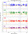 |
Fig. 1 B-V, B-R, V-R, and R-I colors of C/2017 K2 vs. time to perihelion and heliocentric distance, with the mean values from Table 4 compared with the average value of 25 active LPC from Jewitt (2015) (horizontal dashed black lines), and the Sun colors from Holmberg et al. (2006) (horizontal dashed orange lines). The vertical dashed line represents the perihelion, and the vertical dotted blue line represents the water-ice sublimation boundary (~3 au). |
Comparison of the C/2017 K2 colors with those of active LPCs.
Slope fitting results in the light-curve evolution of comet C/2017 K2.
Average logarithmic production rates and A(0)fρ ratios of comet C/2017 K2 in comparison with the A’Hearn et al. (1995) taxonomic classes.
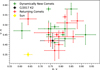 |
Fig. 2 Color–color plot comparing C/2017 K2 (square) with dynamically new comets (green) and returning comets (red) from Jewitt (2015). The color of the Sun is marked by a yellow circle. |
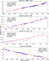 |
Fig. 3 Four different slope regimes in the Rc light curve of comet C/2017 K2. |
3.1.2 Gas production rates, Afρ, and their ratios
Figure 4 illustrates the production rates of several volatile species (OH, NH, C3, CN, and C2) in comet K2. For visibility, the OH production is scaled down by a factor of 10. The logarithmic scale facilitates the comparison of species with different production levels and highlights the changing activity of the comet as it approaches or moves away from the Sun. The production rate values for the various species are summarized in Table A.2. We first detected CN and C2 radicals at the end of March 2022 at 3.62 au, followed by the majority of other radicals that appeared in the coma about a month later, except for NH, which was only observed in mid-August 2022. The production rates gradually increased as the comet approached the Sun, from 3.62 to 2.71 au, and then the rate stabilized surprisingly and showed a plateau-like behavior both before and after perihelion, similar to the optical light curve.
The radical CN remained detectable in our data until midOctober 2023 at 3.88 au, while C2 and C3 were no longer observed after early October at 3.83 au. OH was detected until September 20 at 3.69 au, while NH was detected until the end of March 2023 at 2.20 au. The OH, CN, and C2 values agree well with those of Combi et al. (2025) for the water production rates from SOHO measurements of the Lyman-α H line before and after perihelion and with Schleicher’s narrowband photometric measurements (private communication; see also Figure 4).
We calculated production rate ratios relative to CN and OH, as well as the dust-to-gas ratio. Comet K2 has a log [A(0)fρ/Q(OH)] = –24.75 ± 0.43, which places K2 in the dustrich regime, compared to the typical cometary values (Table 6) reported by A’Hearn et al. (1995). Figure 5 illustrates the evolution of the logarithm of C2/CN over time to the perihelion and heliocentric distances. According to the taxonomic classification by A’Hearn et al. (1995), the comet falls into the typical group, which is defined by a characteristic abundance of C2 and C3 relative to CN and OH. Table 6 summarizes the production rates ratios in K2 compared to the comet database given in A’Hearn et al. (1995).
The apparent magnitude of a comet depends on its heliocentric distance, geocentric distance, and phase angle at the time of observation. To remove geometry and illumination effects, we computed the absolute magnitude (H), defined as the magnitude that the comet would have if it were observed at a heliocentric and geocentric distance of 1 au and a phase angle of 0°. It is given by
 (1)
(1)
where m is the apparent magnitude in a given filter, rh is the heliocentric distance, and rΔ is the geocentric distance. The phase correction f (α) is defined as −2.5log10 [ϕ(α)], where ϕ(α) is the phase function corresponding to the phase angle at the time of observation, as defined in Schleicher et al. (1998). Figure A.2 illustrates the variation in absolute magnitude of comet K2 as a function of days and distance to the perihelion.
The absolute magnitude in the Rc band can be used to derive the effective scattering cross-section (Ce) (Jewitt et al. 2019), which provides insights into the dust content and activity of the comet. It is calculated as
![Mathematical equation: C_e = \frac{\pi r_0^2}{p} \cdot 10^{0.4[m_{\odot,R} - H_R]},](/articles/aa/full_html/2025/09/aa55864-25/aa55864-25-eq3.png) (2)
(2)
where r0 is the mean Earth–Sun distance in km, p is the geometric albedo of the dust, and m⊙,R is the apparent magnitude of the Sun in the Rc band. Using r0 = 1.5 × 10⁸ km and m⊙,R = −26.97 (Willmer 2018), this simplifies Equation (2) to Ce = (1.5 × 10⁶/p) × 10−(0.4HR). We adopted an albedo value of p = 0.04 based on estimates from Jewitt et al. (2019) and Zhang et al. (2019).
The effective scattering cross-section was further used to estimate the average dust-mass loss rate via
 (3)
(3)
where ρ is the bulk density of the dust particles, ā is the mean particle radius, and τr = L/vej is the residence time of the particles within an aperture of radius L, with vej being the ejection velocity. We adopted ρ = 500 kg/m3 and a = 100 μm, following Jewitt et al. (2019). A projected aperture radius of 5" was used for the analysis, corresponding to a physical diameter that varies with the geocentric distance of the comet. Although the dust velocity varies with heliocentric distance, for comparative purposes, we used a fixed ejection velocity of 14 m/s that is consistent with the average velocity for 100 µm grains reported by Liu & Liu (2024).
We analyzed the variation in absolute magnitude, as shown in Figure A.2. K2 displayed an unusual activity pattern as it approached the inner Solar System. Initially, the comet appeared to be exceptionally bright at large distances (~15 au) and had a low absolute magnitude, which suggests strong activity even in the outer Solar System. This brightness was primarily driven by CO sublimation (Meech et al. 2017), which is consistent with the behaviour of the comet between 15 and 13 au, where the absolute magnitude decreased (the comet brightened). The same trend was also reported by Jewitt et al. (2019) for observations at a similar heliocentric range. Below 12 au, however, the absolute magnitude began to increase (the comet became fainter), indicating a decline in CO-driven activity. The most striking feature is the sharp increase in magnitude (fading) between 4 au and 3 au (see the inset in Figure A.2). This can be attributed to the depletion of near-surface CO and/or CO2, which was the main driver of activity until then. Moreover, the nondetection of OH emission in the TRAPPIST and UVES observations before the comet crossed 3 au implies that water (H2O) sublimation had not yet begun, creating a temporary lull in activity. Furthermore, in May (rh=3.23 au), we did not see strong CO and H2O lines in CRIRES+ spectra, which agrees with this hypothesis.
After the comet approached closer than 3 au, the sublimation zone of water ice, the magnitude again started to decrease (brightening), signalling the onset of H2O-driven activity. The comet did not become as bright as expected, however, because water production alone could not compensate for the loss of CO- and CO2- driven activity. The activity trend in A(0)fρ and gas production provides further evidence for this interpretation. Figure 6 shows the evolution of the dust proxy parameter Afρ in cm (A’Hearn et al. 1984) (see Table A.2), measured using the broadband dust continuum filter (Rc), and the narrowband dust continuum filters (RC, GC, and BC). The vertical dashed line marks the comet perihelion at 1.79 au, where A(0)fρ reached a maximum of about 15 000 cm, placing K2 among the very active LPC. Before perihelion, A(0)fρ clearly increased, as is generally normal as the comet approaches the Sun. This reflects the increased dust release as a result of the increased sublimation of ices.
We observed a peculiar behavior between –260 and –170 days to perihelion (3.60 to 2.74 au), however, where Afρ dropped, followed by a rapid increase, suggesting some correlation with the phase angle. This apparently unusual trend persisted even after we accounted for the phase angle, which suggests that the phenomenon is intrinsic to the comet. Furthermore, the water production rate increased sharply around 3 au (see Figure 7), when Afρ and the dust production also started to increase. This might indicate an exhaustion of CO and/or CO2 ice at least in the near-surface layer, which typically drives sublimation activity between 3 and 6 au.
In any case, the comet activity at the time of crossing the snowline clearly underwent a loss of activity, as is visible in the flattening of the light curve and the stalling gas production rates. Kwon et al. (2024) observed the same trend in data from the ZTF IRSA archive5 (Masci et al. 2019) that cover a range from ∼14 to ∼2.3 au. Although the trend is consistent, the Afρ values differ due to variations in photometry that are likely caused by the incorrect zeropoint magnitude information used in their analysis (Kwon et al. 2024, personal communication). Post-perihelion, the Afρ decreases steeply and is not correlated with the phase angle. This behavior is usually observed for LPCs.
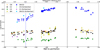 |
Fig. 4 Logarithmic production rates of OH, NH, CN, C2, and C3 of comet C/2017 K2 from TRAPPIST photometry as a function of time and the heliocentric distance. The vertical dashed line indicates the perihelion at 1.79 au on December 19, 2022. |
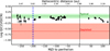 |
Fig. 5 Logarithm of C2/CN production rate ratios of comet C/2017 K2 as a function of time and heliocentric distance. |
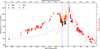 |
Fig. 6 The A(0)fρ parameter of comet C/2017 K2 from the broad- and narrowband filters as a function of time and the heliocentric distance. |
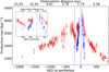 |
Fig. 7 Comparison of dust-mass loss and water-mass production in comet K2 as a function of time and the heliocentric distance. The dust-mass loss was computed using equation (3), and the water-mass production was computed from the OH production rate observed by TRAPPIST. The vertical dotted blue line represents the water-ice sublimation boundary (∼3 au) (Womack et al. 2017; Crovisier & Encrenaz 2000), within which the main driving source of comet outgassing changed from supervolatile ices to H2O ice (Kwon et al. 2023). The vertical dashed line represents the perihelion. |
3.2 High-resolution spectroscopy (VLT)
3.2.1 Optical spectroscopy with UVES
In the first epoch (May 9, 2022, rh=3.23 au), only CN, C3, and C2 were clearly detected with UVES, as in TRAPPIST images. In the second epoch (July 5, rh=2.73 au), OH and all the usual other species started to be detected (NH, CH, and NH2). The emissions became much brighter at the last epoch (Sept 20, rh =2.12 au) (see Figure 8). CO2+ ions were detected, but CO+ ions were never detected, showing that K2 is not a CO+ rich comet like C/2016 R2, which was observed at the same distance and whose optical spectrum was dominated by CO+ bands (Opitom et al. 2019). An observation bias is also possible because we rarely observe CO+ lines in the high-resolution spectra of UVES taken in the last two decades: the slit is usually placed in the bright inner coma where the bands of the neutral species dominate and can hide the faint CO+ lines. The slit is also tiny (10" in length), and geometrically, it might be easy to miss the thin asymmetric CO+ streams (only opposite to the Sun). When the slit is offset from the nucleus in the tail direction, ions can be observed more often.
The production rates of these daughter species were derived from a Haser model (Haser 1957) using the main emission bands (Table 7), and they were simultaneously compared to the parent species that are expected to be detected with CRIRES+. The fluxes are, unfortunately, too weak in the CN lines for us to compute the N and C isotopic ratios.
The high resolution and sensitivity of UVES allowed us to detect the three forbidden [OI] oxygen lines in all three epochs. The green line was detected at 5577.31 Å, and the red doublet was detected at 6300.31 Å and at 6363.78 Å. The Doppler shift that is caused by the velocity of the comet with respect to the Earth separates the comet lines clearly from the strong telluric [OI] lines (see Figure 9). The flux measurements of each line and the so-called green-to-red ratio G/R = I5577/( I6300 + I6364) (Cochran & Cochran 2001) are reported for each epoch in Table 8. The ratio has a clear trend with the heliocentric distance from a rather high value of 0.25 above the water sublimation line at 3.0 au (Crovisier & Encrenaz 2000) to a value close to 0.1 at 2 au, which agrees excellently with the values reported by Decock et al. (2013) and references therein and with Opitom et al. (2019), Cambianica et al. (2021), Cambianica et al. (2023), Kwon et al. (2023), and Aravind et al. (2024) for comets that were observed at various heliocentric distances (see Figure 10). This ratio was commonly used to determine the main parent molecule of the oxygen atoms in the coma, and in particular, the relative contribution of the main comet activity drivers’ H2O, CO2, and CO, as oxygen is mainly produced by the photodissociation of these species (Festou & Feldman 1981). The G/R ratio indeed depends on the progenitor, as shown in Table 2 of Festou & Feldman (1981), with a value of 0.1 for water and higher values for CO and CO2. Submillimeter observations later confirmed carbon monoxide (CO) in the coma of K2 (Yang et al. 2021), and Cambianica et al. (2023) measured a high G/R ratio of 0.28 at 2.8 au. We found a high G/R of 0.25 at 3.2 au, but a lower value of 0.15 at 2.7 au, which agrees well with the average value of 0.15 at 2.53 au from Kwon et al. (2023), who used MUSE at the VLT.
It then rapidly drops to 0.08 at 2.1 au, which agrees with the trend reported by Decock et al. (2013). This illustrates the quick rise of the water sublimation below 3.0 au, which is confirmed by the UVES data, which lack OH lines until the second epoch. These lines are a photodissociation product of H2O. This G/R trend was also observed for several comets at large distances, including K2, and we therefore cannot argue that it was especially rich in CO or CO2 compared to others because an even higher ratio was expected. The nondetection of CO and the detection of CO2+ might indicate that CO2 is the main contributor at heliocentric distances larger than 2.5 au. It would have been very interesting to obtain the ratio at even larger distances than 4.0 au to test this hypothesis.
A recent and surprising discovery was the ubiquitous presence of neutral metallic lines of iron and nickel in high-resolution spectra of comets and detected even far from the Sun (Manfroid et al. 2021). In comet K2, we were able to identify and measure the flux of eight nickel lines and two iron lines in the blue spectra of the last two epochs, sometimes with large uncertainties (see Figure 11 and Table 9). We computed the iron and nickel production rates for the last two epochs: log10(QFe) = 22.01 ± 0.21 (July) and 22.14 ± 0.21 (September) and log10(QNi) = 21.97 ± 0.04 (July), and 22.23 ± 0.08 (September) using the model developed by Manfroid et al. (2021) and Hutsemékers et al. (2021). The ratios for each epochs are then log10(QNi/Fe) = —0.04 ± 0.22 (July) and 0.09 ± 0.23 (September). They agree well within the error bars with the average value for 17 comets of log10(QNi/Fe) = −0.06 ± 0.31, but differ by one order of magnitude from the ratio of −1.10 ± 0.23 estimated in the dust of 1P∕Halley (Jessberger et al. 1988) and −1.11 ± 0.09 measured in the coma of the Sun-grazing comet Ikeya-Seki by Manfroid et al. (2021). Even though it is a DNC and active very far from the Sun, the ratio of NiI/FeI in K2 is similar to that of other comets. As shown in Figure 12, K2 falls in the middle of the correlation found by Hutsemékers et al. (2021) between the level of carbon-chain depletion (C2/CN) and the NiI/FeI ratio of the LPC. This relation suggests that the diversity of NiI/FeI abundance ratios in comets might be related to the cometary formation and not to subsequent processes in the coma.
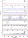 |
Fig. 8 Spectral regions of interest of comet C/2017 K2 acquired with UVES, with detected daughter species in three different epochs: May (rh=3.23 au), July (rh=2.73 au), and September (rh=2.12 au). The flux is reported in arbitrary units for clarity. |
Gas production rates of comet C/2017 K2 from UVES observations.
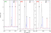 |
Fig. 9 Forbidden green oxygen line [OI] and red doublet lines detected with UVES at the VLT in the three epochs May 9 (rh=3.23 au), July 5 (rh =2.73 au), and September 20 (rh=2.12 au). |
Flux measurements and G/R intensity ratios of the [OI] emission lines for comet C/2017 K2.
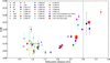 |
Fig. 10 G/R intensity ratio plotted as a function of the heliocentric distance. The same symbol is used for multiple points of a given comet. Open markers represent short-period comets, and solid markers represent LPCs. The vertical dotted line indicates the distance beyond which water sublimation decreases significantly (Crovisier & Encrenaz 2000). |
3.2.2 NIR spectroscopy with CRIRES+
The overall retrieved rotational temperatures, production rates, and mixing ratios (or significant upper limits) we obtained from CRIRES+spectra are reported in Table 11.
Despite the notable activity of the comet even at large heliocentric distances, our infrared observations of K2 reveal a contrasting scenario that is characterized by a very weak dust continuum and faint emission lines from many parent species. Because the dust signal in the infrared is a combination of reflected light and thermal emission, the low dust signal in our IR spectra might arise because the dust is cold: K2 was still quite far away from the Sun, and combined with the dust properties (size, composition, and so on), this might cause the signal to be fainter. Additional simulations are required to properly explain the differences observed between the optical and the infrared. The infrared counterparts of optically detected species, such as H2O, C2H2 and HCN, were barely discernible for the volatile component even when the comet appeared to be bright. This is particularly evident in the spectra taken on May 9, where the CO emission lines are at the noise level and too faint for a proper estimation of the production rate. In the beginning, given the strong activity observed in the optical, we expected spectra that were dominated by hypervolatiles such as CO and CH4. Since this was not the case, we assumed that the comet was still too far from the Sun and the observer to be properly sampled in the infrared. Our later analysis and comparison with TRAPPIST and UVES results instead confirmed a more complex scenario in which our nondetection might most likely be related to a nearsurface depletion of CO before the comet entered the water-ice line (rh < 2.8 au).
In Table 12, we compare our results with those from the recent literature. Our total production rates and mixing ratios are comparable within 2σ with those obtained by Ejeta et al. (2025), with the exception of HCN, for which we obtain a significantly lower value. Similarly, the production rates we measured in July are consistent with those measured by the James Webb Space Telescope (JWST) when the comet was at 2.35 au from the Sun (Woodward et al. 2025), even if the latter reports a water production rate that was twice higher than the rate we measured, and their mixing ratios were accordingly lower.
When compared to other comets, K2 is enriched in almost all the species, and it is similar to C/1999 T1, C/2009 P1, and C/2013 R1 (see Figure 13). A possible scenario that can explain this composition is that the material in this comet formed in a cold environment rich in organics, where CO was particularly abundant and hydrogenation processes on grains contributed significantly to the abundances of species such as methanol, ethane, and methane. Moreover, as a dynamically new comet, K2 most likely preserved its primordial composition during its time in the Oort cloud. This pristine and hypervolatile material has enabled its strong activity even at heliocentric distances larger than 20 au.
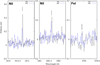 |
Fig. 11 Example of the NiI and FeI lines detected in C/2017 K2. |
Fluxes of NiI and FeI in C/2017 K2.
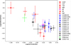 |
Fig. 12 NiI/FeI abundance ratios against the C2/CN adapted from Hutsemékers et al. (2021). The colors in the plot represent different dynamical classes: Jupiter-family comets (red), Halley-family comets (pink), long-period comets (blue), and dynamically new comets (black). The square shows comet C/2017 K2. |
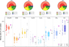 |
Fig. 13 Comparison of K2 with other comets. In the upper panel, the comet is compared with C/2009 P1, C/1999 T1, and C/2013 R1, which show the closest relative abundance proportions. In the bottom plot, we compare K2 (marked with a magenta star) for each species with the box plot statistic from other infrared results relative to comets observed within 2 au from the Sun (Lippi et al. 2021). For each box, the middle line corresponds to the median, the box is limite to the 25th and 75th percentiles, and the whiskers are limited to the 5th and 95th percentiles. C/2009 P1, C/1999 T1, and C/2013 R1 are also shown with a gray square, diamond, and triangle, respectively. |
Abundance ratios derived from the optical and infrared data of comet C/2017 K2.
Production rates and mixing ratios (relative to water) retrieved for the CRIRES+ observations.
Comparison of the total production rates and mixing ratios as retrieved in this work, Ejeta et al. (2025), and Woodward et al. (2025).
3.3 Parent and daughter molecules
To investigate the origin of the radicals observed in the coma of K2, we compared the abundances of the daughter species with the parent molecular species derived from infrared observations using CRIRES+. Table 10 summarizes the abundances of selected radicals observed in the optical and their potential parent species detected in the infrared during the same period. Our CN/OH ratios agree with the HCN/H2O ratios obtained from the infrared observations on approximately the same dates, in particular, on September 21, 2022 (see Table 10). This indicates that HCN is the primary source of the observed CN. The significantly lower C2 abundance compared to C2H6 suggests that C2 is more likely to be dissociated from C2H2 than from C2H6. Previous studies showed that C2 remains associated with both molecules even at large heliocentric distances, as observed in comet Hale-Bopp (Helbert et al. 2005). Furthermore, no clear parent molecule for C3 has been identified in the K2 infrared spectra. This suggests that C3 may be produced by chemical reactions within the coma.
4 Summary and conclusion
We conducted a comprehensive observational analysis of comet C/2017 K2 (PanSTARRS), a dynamically new Oort cloud comet that exhibited activity at a large heliocentric distance. Using data from the TRAPPIST telescopes UVES, and CRIRES+at the VLT, we characterized the long-term evolution of activity and molecular abundances at multiple wavelengths, while the comet approached the Sun. Our TRAPPIST photometric monitoring campaign spanned nearly 8 years and covered the approach to perihelion and the post-perihelion activity of the comet. Over 271 nights of observation, we acquired more than 2204 broadband and 174 narrowband images, and we analyzed the brightness variations and coma properties based on this extensive dataset. The light curve revealed a steady evolution without significant outbursts, and the observed colors remained about the same over a wide range of heliocentric distances.
The narrowband photometric data from TRAPPIST and spectroscopic data obtained from UVES and CRIRES+allowed us to investigate the gas production rates and molecular composition of the coma. CN and C2 radicals were first detected in March 2022, with subsequent detections of other species as the comet moved inward. The production rates increased gradually before perihelion, followed by a stabilization phase. The analysis of relative molecular abundances based on the ratios of C2 and C3 to CN and OH classified K2 as a typical comet, consistent with the taxonomic classification of A’Hearn et al. (1995). Furthermore, our comparison of parent and daughter species confirmed that HCN is the main source of CN, while C2 is likely to be dissociated from C2H2 rather than C2H6.
Our findings show that cometary colors do not provide a clear distinction between different dynamical classes. This is consistent with recent findings by Holt et al. (2024). Notably, comet K2 lies on the bluer end of the color distribution. The temporal evolution of its activity reveals distinct phases that are linked to the sublimation and exhaustion of the surface of various ices. Our analysis of the variation in absolute magnitude, A(0)fρ, and dust production highlighted a peculiar drop in the brightness and dust production between –260 and –170 days of perihelion. This may indicate variations in the sublimation mechanisms of CO and CO2 relative to H2O. The observed trends suggest that the temporary halt in activity was due to the depletion of hypervolatiles in the near-surface layers, and the activity resumed as water sublimation became dominant near perihelion. The switch from a CO2 domination to an H2O dominated coma is also clear from the fast drop in the observed G/R ratio as the comet crossed the water-ice sublimation line at ∼3 au.
In general, our results provide valuable insight into the long-term evolution of comet K2 and its activity. The findings reinforce the idea that CO and other supervolatile species play a significant role in driving cometary activity at large heliocentric distances. In addition, the compositional characteristics of the comet contribute to a broader understanding of dynamically new comets and their evolutionary pathways. Furthermore, our study suggests a possible depletion of the outer layers that are rich in supervolatiles, leading to noticeable changes in the volatile-driven activity as the comet approached the Sun. The existence of a class of comets in which the outermost volatile-rich layers of the nucleus are progressively depleted, resulting in fading of activity, will be further investigated in future works. Future observations of similar objects will help us to refine our understanding of the formation conditions and dynamical history of long-period comets.
Data availability
Table A.2 is available at the CDS via https://cdsarc.cds.unistra.fr/viz-bin/cat/J/A+A/701/A61.
Acknowledgements
This publication uses data products from the TRAPPIST project, under the scientific direction of Emmanuel Jehin, Director of Research at the Belgian National Fund for Scientific Research (F.R.S.-FNRS). TRAPPIST-South is funded by F.R.S.-FNRS under grant PDR T.0120.21, and TRAPPIST-North is funded by the University of Liège in collaboration with Cadi Ayyad University of Marrakech. CRIRES+ and UVES results are based on observations under the program 109.23GX, at the European Southern Observatory, Cerro Paranal. S. Hmiddouch acknowledges funding from the Belgian Academy for Research and Higher Education (ARES). M. Lippi acknowledges funding from the “NextGenerationEU” program, in the context of the Italian “Piano Nazionale di Ripresa e Resilienza (PNRR)”, project code SOE_0000188. M. Vander Don-ckt acknowledges support from the French-speaking Community of Belgium through its FRIA grant. The authors thank NASA, David Schleicher, and the Lowell Observatory for the loan of a set of HB comet filters.
Appendix A Light curve, absolute magnitude evolution, g-factors, gas production rates, and A(0)fρ parameter
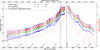 |
Fig. A.1 TRAPPIST Light curve of comet C/2017 K2 measured within a radius aperture of 5-arcseconds as a function of time and distance to perihelion. The vertical dashed line indicates the perihelion at 1.79 au on December 19, 2022. The vertical blue dotted line represents the water ice sublimation boundary (~3 au). |
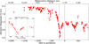 |
Fig. A.2 The absolute magnitude of comet C/2017 K2 as a function of days to perihelion. The vertical blue dotted line represents the water ice sublimation boundary (~3 au) (Womack et al. 2017; Crovisier & Encrenaz 2000), and the dashed line represents the perihelion. The inset is a zoomed-in region of the light curve around 3 au. |
The scale lengths, lifetimes, and the fluorescence efficiencies of the different radicals at 1 au scaled by r−2h.
Appendix B CRIRES+ spectra
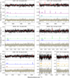 |
Fig. B.1 Spectra of comet C/2017 K2 acquired with CRIRES+. In each plot, the top spectrum shows the observed data along with the total model (in red), while the gray spectrum below represents the modeled transmittance. Molecular models used to derive the production rates are displayed in different colors and labeled accordingly. Residuals are shown at the bottom in gray, with yellow lines indicating the ±1σ uncertainties. Setting, detector number, and observing date are shown on top of each plot. |
References
- A’Hearn, M. F. 1982, in IAU Colloq. 61: Comet Discoveries, Statistics, and Observational Selection, ed. L. L. Wilkening, 433 [Google Scholar]
- A’Hearn, M. F., Schleicher, D. G., Millis, R. L., Feldman, P. D., & Thompson, D. T. 1984, AJ, 89, 579 [Google Scholar]
- A’Hearn, M. F., Millis, R. C., Schleicher, D. O., Osip, D. J., & Birch, P. V. 1995, Icarus, 118, 223 [Google Scholar]
- Aravind, K., Venkataramani, K., Ganesh, S., et al. 2024, MNRAS, 530, 393 [Google Scholar]
- Ballester, P., Modigliani, A., Boitquin, O., et al. 2000, The Messenger, 101, 31 [NASA ADS] [Google Scholar]
- Bessell, M. S. 1990, PASP, 102, 1181 [NASA ADS] [CrossRef] [Google Scholar]
- Bonev, B. P. 2005, PhD thesis, University of Toledo, USA [Google Scholar]
- Cambianica, P., Cremonese, G., Munaretto, G., et al. 2021, A&A, 656, A160 [NASA ADS] [CrossRef] [EDP Sciences] [Google Scholar]
- Cambianica, P., Munaretto, G., Cremonese, G., et al. 2023, A&A, 674, L14 [NASA ADS] [CrossRef] [EDP Sciences] [Google Scholar]
- Cochran, A. L., & Cochran, W. D. 2001, Icarus, 154, 381 [NASA ADS] [CrossRef] [Google Scholar]
- Combi, M., Mäkinen, T., Bertaux, J.-L., Quémerais, E., & Ferron, S. 2025, Icarus, 438, 116645 [Google Scholar]
- Crovisier, J., & Encrenaz, T. 2000, Comet Science: the Study of Remnants from the Birth of the Solar System (Cambridge, UK, New York, USA: Cambridge University Press) [Google Scholar]
- Decock, A., Jehin, E., Hutsemékers, D., & Manfroid, J. 2013, A&A, 555, A34 [NASA ADS] [CrossRef] [EDP Sciences] [Google Scholar]
- Divine, N. 1981, in The Comet Halley. Dust and Gas Environment, eds. B. Battrick, & E. Swallow ESA Special Publication, 174 [Google Scholar]
- Dorn, R. J., Anglada-Escude, G., Baade, D., et al. 2014, The Messenger, 156, 7 [NASA ADS] [Google Scholar]
- Ejeta, C., Gibb, E., DiSanti, M. A., et al. 2025, AJ, 169, 102 [Google Scholar]
- Farnham, T. L., Schleicher, D. G., & A’Hearn, M. F. 2000, Icarus, 147, 180 [Google Scholar]
- Festou, M., & Feldman, P. D. 1981, A&A, 103, 154 [Google Scholar]
- Gomes, R., Levison, H. F., Tsiganis, K., & Morbidelli, A. 2005, Nature, 435, 466 [Google Scholar]
- Hanner, M. S., & Newburn, R. L. 1989, AJ, 97, 254 [Google Scholar]
- Haser, L. 1957, Bull. Soc. Roy. Sci. Liege, 43, 740 [NASA ADS] [Google Scholar]
- Helbert, J., Rauer, H., Boice, D. C., & Huebner, W. F. 2005, A&A, 442, 1107 [NASA ADS] [CrossRef] [EDP Sciences] [Google Scholar]
- Hmiddouch, S., Jehin, E., Jabiri, A., et al. 2024, in European Planetary Science Congress, EPSC2024-1139 [Google Scholar]
- Holmberg, J., Flynn, C., & Portinari, L. 2006, MNRAS, 367, 449 [NASA ADS] [CrossRef] [Google Scholar]
- Holt, C. E., Knight, M. M., Kelley, M. S. P., et al. 2024, PSJ, 5, 273 [Google Scholar]
- Hui, M.-T., Jewitt, D., & Clark, D. 2018, AJ, 155, 25 [Google Scholar]
- Hutsemékers, D., Manfroid, J., Jehin, E., Opitom, C., & Moulane, Y. 2021, A&A, 652, L1 [NASA ADS] [CrossRef] [EDP Sciences] [Google Scholar]
- Jehin, E., Gillon, M., Queloz, D., et al. 2011, The Messenger, 145, 2 [NASA ADS] [Google Scholar]
- Jessberger, E. K., Christoforidis, A., & Kissel, J. 1988, Nature, 332, 691 [Google Scholar]
- Jewitt, D. 2015, AJ, 150, 201 [NASA ADS] [CrossRef] [Google Scholar]
- Jewitt, D., Hui, M.-T., Mutchler, M., et al. 2017, ApJ, 847, L19 [Google Scholar]
- Jewitt, D., Agarwal, J., Hui, M.-T., et al. 2019, AJ, 157, 65 [NASA ADS] [CrossRef] [Google Scholar]
- Jones, G. H., Snodgrass, C., Tubiana, C., et al. 2024, Space Sci. Rev., 220, 9 [NASA ADS] [CrossRef] [Google Scholar]
- Kaeufl, H.-U., Ballester, P., Biereichel, P., et al. 2004, SPIE Conf. Ser., 5492, 1218 [NASA ADS] [Google Scholar]
- Kaiser, N., & Pan-STARRS Team 2002, in American Astronomical Society Meeting Abstracts, 201, 122.07 [Google Scholar]
- Królikowska, M., & Dybczyn´ ski, P. A. 2018, A&A, 615, A170 [NASA ADS] [CrossRef] [EDP Sciences] [Google Scholar]
- Kwon, Y. G., Opitom, C., & Lippi, M. 2023, A&A, 674, A206 [NASA ADS] [CrossRef] [EDP Sciences] [Google Scholar]
- Kwon, Y. G., Bagnulo, S., Markkanen, J., et al. 2024, AJ, 168, 164 [Google Scholar]
- Lippi, M., Villanueva, G. L., Mumma, M. J., et al. 2020, AJ, 159, 157 [Google Scholar]
- Lippi, M., Villanueva, G. L., Mumma, M. J., & Faggi, S. 2021, AJ, 162, 74 [NASA ADS] [CrossRef] [Google Scholar]
- Lippi, M., Vander Donckt, M., Faggi, S., et al. 2023, A&A, 676, A105 [NASA ADS] [CrossRef] [EDP Sciences] [Google Scholar]
- Liu, B., & Liu, X. 2024, A&A, 683, A51 [NASA ADS] [CrossRef] [EDP Sciences] [Google Scholar]
- Manfroid, J., Hutsemékers, D., & Jehin, E. 2021, Nature, 593, 372 [Google Scholar]
- Marcus, J. N. 2007, Int. Comet Q., 29, 39 [Google Scholar]
- Masci, F. J., Laher, R. R., Rusholme, B., et al. 2019, PASP, 131, 018003 [Google Scholar]
- Meech, K. J., Kleyna, J. T., Hainaut, O., et al. 2017, ApJ, 849, L8 [NASA ADS] [CrossRef] [Google Scholar]
- Meier, R., Wellnitz, D., Kim, S. J., & A’Hearn, M. F. 1998, Icarus, 136, 268 [Google Scholar]
- Morbidelli, A., Tsiganis, K., Crida, A., Levison, H. F., & Gomes, R. 2007, AJ, 134, 1790 [NASA ADS] [CrossRef] [Google Scholar]
- Moulane, Y., Jehin, E., Opitom, C., et al. 2018, A&A, 619, A156 [NASA ADS] [CrossRef] [EDP Sciences] [Google Scholar]
- Opitom, C., Jehin, E., Manfroid, J., et al. 2015, A&A, 574, A38 [NASA ADS] [CrossRef] [EDP Sciences] [Google Scholar]
- Opitom, C., Hutsemékers, D., Jehin, E., et al. 2019, A&A, 624, A64 [NASA ADS] [CrossRef] [EDP Sciences] [Google Scholar]
- Paufique, J., Biereichel, P., Donaldson, R., et al. 2004, SPIE Conf. Ser., 5490, 216 [NASA ADS] [Google Scholar]
- Radeva, Y. L., Mumma, M. J., Villanueva, G. L., & A’Hearn, M. F. 2011, ApJ, 729, 135 [NASA ADS] [CrossRef] [Google Scholar]
- Schleicher, D. G. 2010, AJ, 140, 973 [Google Scholar]
- Schleicher, D. G., & A’Hearn, M. F. 1988, ApJ, 331, 1058 [Google Scholar]
- Schleicher, D. G., Millis, R. L., & Birch, P. V. 1998, Icarus, 132, 397 [NASA ADS] [CrossRef] [Google Scholar]
- Villanueva, G. L., Mumma, M. J., DiSanti, M. A., et al. 2011, Icarus, 216, 227 [NASA ADS] [CrossRef] [Google Scholar]
- Villanueva, G. L., Mumma, M. J., Bonev, B. P., et al. 2012, J. Quant. Spec. Radiat. Transf., 113, 202 [Google Scholar]
- Villanueva, G. L., Smith, M. D., Protopapa, S., Faggi, S., & Mandell, A. M. 2018, J. Quant. Spec. Radiat. Transf., 217, 86 [NASA ADS] [CrossRef] [Google Scholar]
- Villanueva, G. L., Liuzzi, G., Faggi, S., et al. 2022, Fundamentals of the Planetary Spectrum Generator [Google Scholar]
- Wainscoat, R. J., Wells, L., Micheli, M., & Sato, H. 2017, Central Bureau Electron. Telegrams, 4393, 1 [Google Scholar]
- Whipple, F. L. 1950, ApJ, 111, 375 [NASA ADS] [CrossRef] [Google Scholar]
- Willmer, C. N. A. 2018, ApJS, 236, 47 [Google Scholar]
- Womack, M., Sarid, G., & Wierzchos, K. 2017, PASP, 129, 031001 [Google Scholar]
- Woodward, C. E., Bockelee-Morvan, D., Harker, D. E., et al. 2025, Planet. Sci. J., 6, 139 [Google Scholar]
- Yang, B., Jewitt, D., Zhao, Y., et al. 2021, ApJ, 914, L17 [NASA ADS] [CrossRef] [Google Scholar]
- Zhang, X. L., Jewitt, D., & Hui, M. T. 2019, MNRAS, 487, 2919 [Google Scholar]
- Zhang, Q., Kolokolova, L., Ye, Q., & Vissapragada, S. 2022, PSJ, 3, 135 [NASA ADS] [Google Scholar]
All Tables
Simultaneous UVES and CRIRES+ observational circumstances of comet C/2017 K2, with the UT2 and UT3 telescopes of the ESO VLT.
Average logarithmic production rates and A(0)fρ ratios of comet C/2017 K2 in comparison with the A’Hearn et al. (1995) taxonomic classes.
Flux measurements and G/R intensity ratios of the [OI] emission lines for comet C/2017 K2.
Production rates and mixing ratios (relative to water) retrieved for the CRIRES+ observations.
Comparison of the total production rates and mixing ratios as retrieved in this work, Ejeta et al. (2025), and Woodward et al. (2025).
The scale lengths, lifetimes, and the fluorescence efficiencies of the different radicals at 1 au scaled by r−2h.
All Figures
|
Fig. 1 B-V, B-R, V-R, and R-I colors of C/2017 K2 vs. time to perihelion and heliocentric distance, with the mean values from Table 4 compared with the average value of 25 active LPC from Jewitt (2015) (horizontal dashed black lines), and the Sun colors from Holmberg et al. (2006) (horizontal dashed orange lines). The vertical dashed line represents the perihelion, and the vertical dotted blue line represents the water-ice sublimation boundary (~3 au). |
| In the text | |
|
Fig. 2 Color–color plot comparing C/2017 K2 (square) with dynamically new comets (green) and returning comets (red) from Jewitt (2015). The color of the Sun is marked by a yellow circle. |
| In the text | |
|
Fig. 3 Four different slope regimes in the Rc light curve of comet C/2017 K2. |
| In the text | |
|
Fig. 4 Logarithmic production rates of OH, NH, CN, C2, and C3 of comet C/2017 K2 from TRAPPIST photometry as a function of time and the heliocentric distance. The vertical dashed line indicates the perihelion at 1.79 au on December 19, 2022. |
| In the text | |
|
Fig. 5 Logarithm of C2/CN production rate ratios of comet C/2017 K2 as a function of time and heliocentric distance. |
| In the text | |
|
Fig. 6 The A(0)fρ parameter of comet C/2017 K2 from the broad- and narrowband filters as a function of time and the heliocentric distance. |
| In the text | |
|
Fig. 7 Comparison of dust-mass loss and water-mass production in comet K2 as a function of time and the heliocentric distance. The dust-mass loss was computed using equation (3), and the water-mass production was computed from the OH production rate observed by TRAPPIST. The vertical dotted blue line represents the water-ice sublimation boundary (∼3 au) (Womack et al. 2017; Crovisier & Encrenaz 2000), within which the main driving source of comet outgassing changed from supervolatile ices to H2O ice (Kwon et al. 2023). The vertical dashed line represents the perihelion. |
| In the text | |
|
Fig. 8 Spectral regions of interest of comet C/2017 K2 acquired with UVES, with detected daughter species in three different epochs: May (rh=3.23 au), July (rh=2.73 au), and September (rh=2.12 au). The flux is reported in arbitrary units for clarity. |
| In the text | |
|
Fig. 9 Forbidden green oxygen line [OI] and red doublet lines detected with UVES at the VLT in the three epochs May 9 (rh=3.23 au), July 5 (rh =2.73 au), and September 20 (rh=2.12 au). |
| In the text | |
|
Fig. 10 G/R intensity ratio plotted as a function of the heliocentric distance. The same symbol is used for multiple points of a given comet. Open markers represent short-period comets, and solid markers represent LPCs. The vertical dotted line indicates the distance beyond which water sublimation decreases significantly (Crovisier & Encrenaz 2000). |
| In the text | |
|
Fig. 11 Example of the NiI and FeI lines detected in C/2017 K2. |
| In the text | |
|
Fig. 12 NiI/FeI abundance ratios against the C2/CN adapted from Hutsemékers et al. (2021). The colors in the plot represent different dynamical classes: Jupiter-family comets (red), Halley-family comets (pink), long-period comets (blue), and dynamically new comets (black). The square shows comet C/2017 K2. |
| In the text | |
|
Fig. 13 Comparison of K2 with other comets. In the upper panel, the comet is compared with C/2009 P1, C/1999 T1, and C/2013 R1, which show the closest relative abundance proportions. In the bottom plot, we compare K2 (marked with a magenta star) for each species with the box plot statistic from other infrared results relative to comets observed within 2 au from the Sun (Lippi et al. 2021). For each box, the middle line corresponds to the median, the box is limite to the 25th and 75th percentiles, and the whiskers are limited to the 5th and 95th percentiles. C/2009 P1, C/1999 T1, and C/2013 R1 are also shown with a gray square, diamond, and triangle, respectively. |
| In the text | |
|
Fig. A.1 TRAPPIST Light curve of comet C/2017 K2 measured within a radius aperture of 5-arcseconds as a function of time and distance to perihelion. The vertical dashed line indicates the perihelion at 1.79 au on December 19, 2022. The vertical blue dotted line represents the water ice sublimation boundary (~3 au). |
| In the text | |
|
Fig. A.2 The absolute magnitude of comet C/2017 K2 as a function of days to perihelion. The vertical blue dotted line represents the water ice sublimation boundary (~3 au) (Womack et al. 2017; Crovisier & Encrenaz 2000), and the dashed line represents the perihelion. The inset is a zoomed-in region of the light curve around 3 au. |
| In the text | |
|
Fig. B.1 Spectra of comet C/2017 K2 acquired with CRIRES+. In each plot, the top spectrum shows the observed data along with the total model (in red), while the gray spectrum below represents the modeled transmittance. Molecular models used to derive the production rates are displayed in different colors and labeled accordingly. Residuals are shown at the bottom in gray, with yellow lines indicating the ±1σ uncertainties. Setting, detector number, and observing date are shown on top of each plot. |
| In the text | |
Current usage metrics show cumulative count of Article Views (full-text article views including HTML views, PDF and ePub downloads, according to the available data) and Abstracts Views on Vision4Press platform.
Data correspond to usage on the plateform after 2015. The current usage metrics is available 48-96 hours after online publication and is updated daily on week days.
Initial download of the metrics may take a while.