| Issue |
A&A
Volume 701, September 2025
|
|
|---|---|---|
| Article Number | A284 | |
| Number of page(s) | 13 | |
| Section | Cosmology (including clusters of galaxies) | |
| DOI | https://doi.org/10.1051/0004-6361/202555887 | |
| Published online | 26 September 2025 | |
syren-baryon: Analytic emulators for the impact of baryons on the matter power spectrum
1
Heuristic and Evolutionary Algorithms Laboratory, University of Applied Sciences Upper Austria, Hagenberg, Austria
2
CNRS & Sorbonne Université, Institut d’Astrophysique de Paris (IAP), UMR 7095, 98 bis bd Arago, F-75014 Paris, France
3
Astrophysics, University of Oxford, Denys Wilkinson Building, Keble Road, Oxford OX1 3RH, UK
4
Institute of Cosmology & Gravitation, University of Portsmouth, Dennis Sciama Building, Portsmouth PO1 3FX, UK
⋆ Corresponding authors: This email address is being protected from spambots. You need JavaScript enabled to view it.
; This email address is being protected from spambots. You need JavaScript enabled to view it.
Received:
10
June
2025
Accepted:
5
August
2025
Abstract
Context. Baryonic physics has a considerable impact on the distribution of matter in our Universe on scales probed by current and future cosmological surveys, acting as a key systematic in such analyses.
Aims. We seek simple symbolic parametrisations for the impact of baryonic physics on the matter power spectrum for a range of physically motivated models, as a function of wavenumber, redshift, cosmology, and parameters controlling the baryonic feedback.
Methods. We used symbolic regression to construct analytic approximations for the ratio of the matter power spectrum in the presence of baryons to that without such effects. We obtained separate functions of each of four distinct sub-grid prescriptions of baryonic physics from the CAMELS suite of hydrodynamical simulations (Astrid, IllustrisTNG, SIMBA, and Swift-EAGLE) as well as for a baryonification algorithm. We also provide functions that describe the uncertainty on these predictions, due to both the stochastic nature of baryonic physics and the errors on our fits.
Results. The error on our approximations to the hydrodynamical simulations is comparable to the sample variance estimated through varying initial conditions, and our baryonification expression has a root mean squared error of better than one percent, although this increases on small scales. These errors are comparable to those of previous numerical emulators for these models. Our expressions are enforced to have the physically correct behaviour on large scales and at high redshift. Due to their analytic form, we are able to directly interpret the impact of varying cosmology and feedback parameters, and we can identify parameters that have little to no effect.
Conlcusions. Each function is based on a different implementation of baryonic physics, and can therefore be used to discriminate between these models when applied to real data. We provide a publicly available code for all symbolic approximations found.
Key words: hydrodynamics / methods: numerical / cosmological parameters / cosmology: theory / dark energy / large-scale structure of Universe
© The Authors 2025
 Open Access article, published by EDP Sciences, under the terms of the Creative Commons Attribution License (https://creativecommons.org/licenses/by/4.0), which permits unrestricted use, distribution, and reproduction in any medium, provided the original work is properly cited.
This article is published in open access under the Subscribe to Open model. This email address is being protected from spambots. You need JavaScript enabled to view it. to support open access publication.
1. Introduction
It is now clear that galaxy formation or, more generally, baryons, can play a significant role in the morphology and evolution of the large-scale structure of the Universe (Chisari et al. 2018). The intricate interplay between gravitational collapse and feedback processes due to supernova explosions and active galactic nuclei (AGNs) can determine the amplitude of clustering on small to intermediate scales. This, in turn, means that, if one is to continue to use large-scale structure as an accurate probe of fundamental physics, one must take into account the role of baryons and how their effects might contaminate the accuracy of cosmological constraints (Amon & Efstathiou 2022; Preston et al. 2023). Alternatively, one can view the statistics of the large-scale structure of the Universe as a new window onto the complex processes that are at play in galaxy formation.
While there have been significant steps in understanding galaxy formation and evolution, fuelled by observations from new observatories, it is still an open problem. From observations, there is not yet a consensus as to whether baryonic effects are large (Hadzhiyska et al. 2024; Bigwood et al. 2024), moderate (Lu & Haiman 2021; Chen et al. 2023), or small (Terasawa et al. 2025; García-García et al. 2024). From a theoretical point of view, the study of galaxy formation relies heavily on computer simulations that attempt to take into account a plethora of physical processes over a vast range of scales. Given the computational limitations, approximations have to be made on small scales, attempting to accurately model the effects of baryons on scales below the resolution of the simulation. The choices made for the ‘sub-grid’ physics can play a crucial role in the outcome of cosmological simulations, with different choices (by different research groups) leading to significantly different outcomes (Chisari et al. 2018).
Our focus is on the effect of baryons, and the large uncertainties in their modelling, on two-point clustering statistics, specifically, the power spectrum of matter fluctuations. We define it as follows. Given a density of matter, ρM(t, x), at a time, t, and spatial co-ordinates, x, we can define the density contrast, δM, through ![Mathematical equation: $ \rho_{\mathrm{M}}={\bar \rho}_{\mathrm{M}}[1+\delta_{\mathrm{M}}(t,\mathbf{x})] $](/articles/aa/full_html/2025/09/aa55887-25/aa55887-25-eq1.gif) , where
, where  is the mean matter density at time t. If, at a fixed time, t, we take the spatial Fourier transform of the density contrast, we obtain δM(k) (where, for ease of notation, the dependence on t is implicit and k is the wavenumber). Assuming that the inhomogeneities in ρM are statistically homogeneous and isotropic, we can define the power spectrum, PM(k), to be
 (1)
(1)
where δ3(⋯) is the 3D Dirac delta function. The shape and amplitude of the power spectrum, P(k), characterise the large-scale structure of the Universe and are sensitive to cosmological parameters such as the expansion rate, the fractional density of different components, the initial conditions, the mass of neutrinos, and other such fundamental properties. It is its sensitivity to baryonic physics that we wish to characterise here.
There has been a considerable amount of work on the effect of baryons on clustering. Early on, baryon cooling (White 2004) and the effects of hot intercluster gas (Zhan & Knox 2004) were shown to play an important role, as was the impact of AGN feedback on P(k) (van Daalen et al. 2011). The first attempts at quantifying the impact of baryons on the matter power spectrum from the OverWhelmingly Large Simulations (OWLS) suite (Schaye et al. 2010) were then applied to data (Köhlinger et al. 2016, 2017; Hikage et al. 2019), showing that small-scale information has a significant impact on both cosmological and baryonic constraints. In parallel, there has been an ongoing programme to incorporate the effect of baryons into models of clustering, either through the halo model (Semboloni et al. 2011; Fedeli 2014; Fedeli et al. 2014; Mohammed et al. 2014; Semboloni et al. 2011, 2013; Debackere et al. 2020) and variants of it (Mead et al. 2015, 2021; Lu & Haiman 2021), effective field theory methods (Lewandowski et al. 2015; Bragança et al. 2021; Sullivan et al. 2021), through the process of ‘baryonification’ (Schneider & Teyssier 2015; Schneider et al. 2019, 2020; Aricò et al. 2020) applied directly to N-body simulations and mock data, and through the use of machine learning (Tröster et al. 2019; Villaescusa-Navarro et al. 2022). More recently, more targeted simulations focussing on smaller scales have looked at the role black holes may play in baryonic processes (Martin-Alvarez et al. 2024). While the inference of the impact of baryons on structure formation can be very sensitive to assumptions of a given hydrodynamical simulation (Villaescusa-Navarro et al. 2021a; Villanueva-Domingo & Villaescusa-Navarro 2022; Delgado et al. 2023), it has been shown that reasonably robust observable quantities can be constructed (Shao et al. 2023; Wadekar et al. 2023a; Villanueva-Domingo et al. 2022; Villaescusa-Navarro et al. 2021b; Wadekar et al. 2023b; Jo et al. 2025).
A general trend has developed of constructing surrogates or ‘emulators’ that can, efficiently and accurately, reproduce the impact of baryonic physics on large-scale structure through the use of machine learning techniques. These involve the use of principle component analysis (Huang et al. 2019; Eifler et al. 2015; Foreman et al. 2016), Gaussian processes (Sharma et al. 2025; Giri & Schneider 2021), random forest methods (Delgado et al. 2023), enthalpy gradient descent schemes (Dai et al. 2018) and, most notably, neural networks (Aricò et al. 2021a). In the case of neural networks, these have been used to explore the impact of baryons on cosmological constraints from current data using small scales (Aricò et al. 2023; García-García et al. 2024).
In this work, instead of leveraging these numerical machine learning techniques, we employ the supervised machine learning technique of symbolic regression (Kronberger et al. 2024), which attempts to learn concise and accurate symbolic approximations directly from a dataset. This technique has been successfully applied to achieve percent-level-accurate SYmbolic Regression ENhanced (SYREN) emulators of the matter power spectrum in the absence of baryons (Bartlett et al. 2024a,b; Sui et al. 2025), so this works extends these approximations to capture their effect; we name the set of models produced ‘SYREN-BARYON’.
To characterise the effects of various models of baryonic feedback on the distribution of matter in the Universe, we wish to find symbolic approximations to the function
 (2)
(2)
where k is the wavenumber, z is the redshift, and θ is a vector of cosmological and/or astrophysical parameters. P(k, z, θ) is the matter power spectrum in the presence of baryons, and Pnbody(k, z, θ) is the corresponding quantity for a ‘N-body’ scenario, i.e. in the absence of all astrophysical processes where the only force is gravity. Sharma et al. (2025) showed that this is the only quantity required to model baryonic effects at the field level up to scales k ∼ 10 h Mpc−1 due to the large cross-correlation between fields with and without astrophysical effects.
Through causality, baryons cannot have effects on the very largest scales, and thus we require that S(k, z, θ) → 1 as k → 0 for any z and θ. However, for other values of k, the shape of S(k, z, θ) is determined entirely by the model used to describe baryonic processes in the Universe, and can be very sensitive to this choice (Chisari et al. 2018). In this paper we consider broadly two classes of baryonic models: hydrodynamical simulations and baryonification algorithms, which are described in Sections 2.1 and 2.2, respectively. We consider four different hydrodynamical simulations and a single baryonification model, and thus derive five different functions for S(k, z, θ). We choose to emulate the baryonification model of Aricò et al. (2020), although note that we could have equally chosen the Schneider & Teyssier (2015) model, which has a numerical emulator (Giri & Schneider 2021). By comparing our functions to observations, one could constrain the parameters of these models and, through Bayesian model comparison, determine which of these gives the most faithful representation of baryonic physics at the level of the power spectrum, given current data.
The paper is organised as follows. In Section 2 we describe the implementations of baryonic physics we consider and the different loss functions used for the hydrodynamical simulations versus the baryonification model. Section 3 describes the search for analytic approximations to S(k, z, θ) with symbolic regression and how we choose which model to select. These expressions are then presented in Section 4 and discussed in Section 5. We conclude in Section 6. The main results of the paper are summarised in Tables 3 and 4. Throughout, we use ‘log’ to denote the natural logarithm, with base-10 logarithms written as ‘log10’. Whenever the wavenumber, k, appears in a mathematical expression, it is assumed to have units of h Mpc−1.
2. Baryon models
2.1. Hydrodynamical simulations
Our current understanding of galaxy formation and evolution has been improved greatly thanks to large-scale cosmological hydrodynamic simulations (Davé et al. 2019; Nelson et al. 2019; Dubois et al. 2014; Schaye et al. 2015; Vogelsberger et al. 2014; Lee et al. 2021; Vogelsberger et al. 2020; McCarthy et al. 2017; Bassini et al. 2020; Feng et al. 2016; Dolag et al. 2017). These simulations can reproduce galaxies that align well with observations in various aspects such as mass distributions, structures, and colours thanks to their detailed modelling of baryonic processes. However, due to the finite resolution of the simulations, many critical astrophysical mechanisms cannot be resolved, and thus one must rely on sub-grid models for processes such as star formation, the growth of supermassive black holes, stellar feedback, and AGN feedback. These remain poorly understood, and therefore often require extensive tuning of parameters to match observational data (Somerville & Davé 2015), which poses limitations on their application in precision cosmological analyses.
Instead of having a single cosmological simulation with tuned hydrodynamical parameters, the Cosmology and Astrophysics with MachinE Learning Simulations (CAMELS) (Villaescusa-Navarro et al. 2021a, 2023; Ni et al. 2023) project provides a suite of hydrodynamical simulations with varying cosmological and astrophysical parameters. This enables one to see the effect of such variation and is designed as a machine learning training set, so that one can either infer or marginalise over these parameters when applied to real data.
For this work, we focus on two sub-sets of the CAMELS suite, both of which are run from redshift z = 127 to z = 0, and are conducted in a periodic comoving volume of length 25 h−1 Mpc with 2563 dark matter particles and, for those involving hydrodynamics, 2563 initial gas resolution elements. Firstly, we consider the Latin Hypercube (LH) of simulations. These consist of 1000 simulations where the cosmological and astrophysical parameters are varied across a LH in the range given in Table 1. In particular, Ωm and σ8 are allowed to vary across a large range, with all other cosmological parameters fixed to Ωb = 0.049, h = 0.6711, ns = 0.9624, Mν = 0 eV, w0 = −1, wa = 0, ΩK = 0. The four astrophysical parameters that are allowed to vary (ASN1, ASN2, AAGN1, AAGN2) are related to stellar and AGN feedback, and are scaled such that a value of unity corresponds to the original implementation of the simulations considered. We use 80 % of these simulations for training our models and the remaining 20 % for testing.
Range of the cosmological (upper) and hydrodynamical (lower) parameters used in the CAMELS simulations considered.
Given the uncertainty in how to model unresolved astrophysical processes, the CAMELS suite provides simulations with different sub-grid models. In this work, we consider the four models for which – at the time of writing – contain 1000 publicly available LH simulations and wish to find a different function for S(k, z, θ) for each prescription. These are:
-
Astrid: These simulations are run using the MP-Gadget code (Springel et al. 2021) with the Astrid sub-grid physics model (Ni et al. 2022; Bird et al. 2012).
-
IllustrisTNG: This suite utilises the Arepo code (Springel 2010; Weinberger et al. 2020) and employs the IllustrisTNG model of galaxy formation. This model is fully described in Weinberger et al. (2017), Pillepich et al. (2018), where the data release for the fiducial simulation is provided in Nelson et al. (2019).
-
SIMBA: For these simulations, the SIMBA model (Davé et al. 2019) of galaxy formation is used, and these are run using the GIZMO code (Hopkins 2015).
-
Swift-EAGLE: This suite is an implementation of the EAGLE sub-grid model (Schaye et al. 2015; Crain et al. 2015) within the Swift code (Schaller et al. 2024).
For a thorough description of these simulations, see the CAMELS papers (Villaescusa-Navarro et al. 2021a, 2023; Ni et al. 2023) and references therein. It is important to note that the meaning of the baryonic physics parameters (ASN1, ASN2, AAGN1, AAGN2) depends on the simulation considered, and therefore these cannot be directly compared across the simulations (see Table 1 of Lovell et al. 2024, for a succinct summary of the meaning of these parameters in the different simulations).
As well as the LH set, for each sub-grid model and N-body code, there is a set of 27 simulations that take a fiducial set of cosmological and astrophysical parameters (Ωm = 0.3, σ8 = 0.8, ASN1 = ASN2 = AAGN1 = AAGN2 = 1), and sample the effect of cosmic variance (CV) using different initial random seeds. Although the cosmic variance for a pure N-body simulation would be small on these scales, different initial conditions can dramatically affect the astrophysical processes that occur, and thus a substantial variation in the power spectrum can be observed, particularly given the relatively small box sizes of the CAMELS simulations. This is depicted in Fig. 1, where we see that, on large scales, all CV simulations predict the same power spectrum, but on small scales the effects of varying initial conditions and the stochastic nature of baryonic feedback can yield significantly different power spectra.
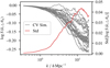 |
Fig. 1. Baryonic effect, log S (Eq. (2)), on the power spectrum for the 27 CV simulations and its standard deviation over k for the Astrid sub-grid model at z = 0. |
We used the CV simulations to estimate the sample variance of S(k, z, θ) by defining the variable
![Mathematical equation: $$ \begin{aligned} \sigma (k, z) = \max \left( 0.01, \underset{\mathrm{CV}}{\mathrm{Std}} \left[ \log S(k, z, \boldsymbol{\theta }_\star ) \right] \right), \end{aligned} $$](/articles/aa/full_html/2025/09/aa55887-25/aa55887-25-eq5.gif) (3)
(3)
where Std denotes the standard deviation, which we computed over the CV simulations at fixed k and z, and θ⋆ are the model parameters of the CV suite. We chose a lower bound of 0.01 since we are aiming for (at best) percent-level accuracy in our predictions, so are content with widening the error bars at values of k for which the variation across the CV set is smaller than this. σ(k, z) has significant scale dependence, as demonstrated by the red line in Fig. 1. This is to be expected physically since, through causality, the very largest scales cannot be affected by feedback and the effects of cosmic variance on the dark-matter-only power spectrum have been divided out by computing S. Similarly, σ(k, z) is smaller at higher redshift since there has been less time for baryonic processes to impact the matter distribution, and thus all simulations have similar power spectra.
One should expect that σ depends on cosmological and astrophysical parameters, since, in the extreme case where there is no baryonic feedback, the simulations are identical to the N-body suite, and thus the value of S would be unity independent of k, z or the initial conditions of the simulation; the standard deviation over the CV set would then be zero. However, since we only have a CV suite at the fiducial parameters, we are forced to assume that the errors are independent of these variables. This is common practice in cosmological analyses, where covariance matrices are typically computed at a fiducial set of cosmological parameters (Kodwani et al. 2019).
Given the noisy estimate of S(k, z,θ) from a single simulation and its strong dependence on k, instead of using a mean squared error loss for our symbolic expressions, we minimise
![Mathematical equation: $$ \begin{aligned} - \log \mathcal{L} [S_{\rm pred} ] = \sum _{i \in \mathrm{LH}} \sum _{k,z} \frac{\left( \log S(k, z, \boldsymbol{\theta }_i) - \log S_{\rm pred}(k, z, \boldsymbol{\theta }_i)\right)^2}{2 \sigma ^2 (k,z)}, \end{aligned} $$](/articles/aa/full_html/2025/09/aa55887-25/aa55887-25-eq6.gif) (4)
(4)
where S(k, z, θi) is computed from simulation number i on the LH, and Spred(k, z, θi) is a candidate symbolic expression. In fact, for numerical convenience, we do not directly optimise logℒ but the normalised mean squared error, such that
![Mathematical equation: $$ \begin{aligned} \mathrm{NMSE} \equiv \frac{\log \mathcal{L} [S_{\rm pred} ]}{\log \mathcal{L} [\bar{S}]}, \end{aligned} $$](/articles/aa/full_html/2025/09/aa55887-25/aa55887-25-eq7.gif) (5)
(5)
where we define  to be the mean of log S over k, z and θ.
We used 25 values of k, logarithmically spaced in the range 0.35 − 19.97 h Mpc−1, and 12 redshift values ![Mathematical equation: $ z \in [0.00, \, 0.05, \, 0.10, 0.15, 0.21, 0.34, 0.54, 0.95, 1.48, 2.46, \, 4.01, \, 127.0] $](/articles/aa/full_html/2025/09/aa55887-25/aa55887-25-eq9.gif) . To compute S(k, z, θ), we utilised the publicly available P(k, z, θ) and Pnbody(k, z, θ), which were originally obtained using the PYLIANS code (Villaescusa-Navarro 2018). This loss function ensures that our expressions are better fitting at low k and z where the uncertainty from the simulation is lower.
. To compute S(k, z, θ), we utilised the publicly available P(k, z, θ) and Pnbody(k, z, θ), which were originally obtained using the PYLIANS code (Villaescusa-Navarro 2018). This loss function ensures that our expressions are better fitting at low k and z where the uncertainty from the simulation is lower.
2.2. Baryonification
Instead of incorporating hydrodynamics into the simulation itself, an alternative approach is to first run a N-body, dark-matter-only simulation (which requires a much lower computational budget), and then augment the output to correct for this missing physics. This approach – baryonification (Schneider & Teyssier 2015; Schneider et al. 2019; Aricò et al. 2020) – perturbs the final positions of the dark matter particles under a set physically motivated prescriptions for effects such as star formation, gas cooling, and AGN feedback. As such, the power spectrum is modified due to the impact of baryons.
In particular, we wish to emulate this effect under the model of Aricò et al. (2020). In this case, the dark matter is assumed to quasi-adiabatically relax under the modification of the gravitational potential caused by the baryonic mass components. Central galaxies are assumed to have mass profiles given by an exponentially decaying power law that is fixed to r−2. Their masses are set by halo abundance matching. These are surrounded by satellite galaxies of 20% of the mass of the central, and are distributed according the dark matter profile. Gas is assumed to be bound in halos, with a distribution given by a double power law, where the transition and slopes are free parameters. Some of the gas is ejected, and is modelled as a constant density with an exponential cut-off with characteristic scale η. The mass fraction of these two gas components is given by a parametric function of the host halo mass, and the total stellar and gas mass is designed to equal the cosmic density of baryons.
This model is described by seven parameters, and we allow these to vary in the ranges given by Table 2. The density profiles of hot gas in halos are given by θinn, Minn and θout with a mass fraction given by Mc and β. The extent of the ejected gas is given by η and the characteristic halo mass scale for centrals is determined by M1. These prior ranges were chosen to match that of Aricò et al. (2021a) and are similar to those of Aricò et al. (2021b) since these are sufficiently wide to reproduce the clustering of several hydrodynamic simulations. In Table 2 we also state the values chosen for these parameters in our fiducial case, which we will use to visualise the results of our symbolic fits.
Ranges of the cosmological (upper) and baryonification (lower) parameters used and their fiducial values.
For computational convenience, instead of generating new suites of N-body simulations with the cosmological parameters drawn from the ranges given in Table 2 and then adjusting these using sampled values of the baryonification parameters, we utilised the BACCO emulator (Aricò et al. 2021a). This emulator can reproduce S(k, θ) with percent-level precision across the desired parameter range and redshifts, and thus is sufficiently accurate for our purposes.
We generated two sets of 1000 simulations with 50 values of k each for training and testing, and parameters drawn from a LH. Values for k are logarithmically spaced in the range 0.01 − 4.692 h Mpc−1. Redshifts are uniformly sampled in the range of 0 − 1.5 as the BACCO emulator does not support higher values. Since we did not have access to a measure of uncertainty on these power spectra, we minimised the following normalised mean squared error:
 (6)
(6)
which is identical to Eq. (5) for constant σ(k, z).
3. Symbolic regression
To find simple but accurate descriptions of baryonic effects on the power spectrum, we used the supervised machine learning technique of symbolic regression (SR) (Kronberger et al. 2024). We employed the genetic programming-based SR code OPERON (Burlacu et al. 2020), which utilises evolutionary processes inspired by natural selection, including crossover (breeding) and mutation, to develop an initial set of functions over successive generations. This method ensures that well-fitting and simple expressions are retained, while those that are poorly fitting or overly complex are eliminated. Consequently, after several iterations, a refined population of expressions that accurately approximate the dataset is produced. We selected OPERON over other SR tools because of its superior performance in benchmark evaluations (Cava et al. 2021; Burlacu 2023) and its proven effectiveness in cosmological and astrophysical research (Bartlett et al. 2024a,b; Sui et al. 2025; AbdusSalam et al. 2025).
Free parameters in the expressions evaluated by OPERON are optimised (Kommenda et al. 2020) using the Levenberg–Marquardt algorithm (Levenberg 1944; Marquardt 1963). This includes additional scaling parameters, which are present at each terminal node within the expression tree. The model length is defined as the number of nodes in an expression tree, excluding these scaling terms. During the non-dominated sorting process, the objective values (the accuracy metric and model length relative to the maximum model length) of the equations are compared using ϵ-dominance (Laumanns et al. 2002). Here, a hyper-parameter ϵ is supplied to OPERON, so that two objective values within an ϵ distance of each other are considered equivalent, which helps the algorithm converge. We chose ϵ = 10−7. We only used arithmetic functions (+, ×, ÷, pow) and the chosen maximum model size (maximum model length of 60 and expression tree depth of 10) because we observed that non-linear functions in the function set, as well as allowing larger models, led to models with implausible structure or discontinuities within the given variable value ranges. We terminated the search after 1000 generations because OPERON did not find any improvements after around 500–600 generations. We set the mutation rate (25%), as well as the population size (1000) and selection procedure (tournament; group size = 5) to their default values.
To choose a model, we considered the error on the test dataset, the model complexity, and prior knowledge of the behaviour of our model at large scales and early times. In particular, we required two physically motivated constraints:
-
S(k, z, θ) → 1 as k → 0 for any z and θ: On the largest scales, by causality arguments, baryons cannot have an effect, and thus the matter power spectrum must be equal to the dark-matter-only prediction.
-
S(k, z, θ) → 1 as z → ∞ for any k and θ: At high redshift, there has been insufficient time for baryonic processes to disrupt the matter distribution, and thus the matter power spectrum should be the same with or without baryons included.
We calculated the Pareto front of the test error and the model length and selected the model with the lowest error that analytically satisfies these constraints. Since the structure of the chosen model occurs often multiple times in the final population with different parameters, we selected the model structure with the parameters that minimise the description length (Bartlett et al. 2023) for hydrodynamical simulations. For the baryonification model, we only used the NMSE as an error measure, as there is no uncertainty in the data. Given that k starts at 0.35 h Mpc−1, we added data for low S(k = 0.01 h Mpc−1, z, θ) for all z and θ in the training set of all the hydrodynamical simulations to guide the optimisation procedure towards solutions that satisfy the constraints in respect of k. For the hydrodynamical simulations, we corrected any remaining bias on the training set over all values of θ parameters with a separate function of k and z, which is summed with our original model of log S(k, z, θ). We approximated the bias again with OPERON in the same way as the original function, but with a smaller tree size (maximum expression tree depth of 6 and maximum model length of 25) and a function set including exponentiation. We selected the model with the lowest error that analytically satisfies the constraints from a Pareto front of model length and test error.
Not only do we wish to provide fits for S(k, z, θ), but also on the typical error on the prediction. This error arises due to an intrinsic scatter due to sample variance (Fig. 1), but also due to imperfect symbolic fits. Including this theoretical covariance within cosmological analyses has been shown to reduce biases in cosmological parameters without requiring strict scale-cuts (Maraio et al. 2025). We model this error ε (defined as half of the range of 68% of the error at each k and z) as a function of k and z. Given the two physically motivated constraints for S(k, z, θ) are enforced to hold exactly, this yields the following corresponding constraints on the error
-
ε(k, z)→0 as k → 0.
-
ε(k, z)→0 as z → ∞.
We used OPERON to model ε with the settings described above but a maximum expression tree depth of 7, a maximum model length of 30, and a function set with exponentiation. Since the constraints are not enforced during OPERON’s search, we used them for model selection from OPERON’s Pareto front of model length and test error. We selected the model with the lowest error that satisfies these constraints. For all expressions, we repeated the search five times with different initial random seeds to ensure that it did not converge to local minima with insufficient accuracy, implausible structures, or constraint violations regarding k and z.
4. Results
After running OPERON for each of the baryonic physics models, we obtain the Pareto fronts plotted in Fig. A.1. For all of the models, we see that the training and validation losses are relatively similar, suggesting that our models have not over-fitted on the training set. For the hydrodynamical simulations, we find that the NMSE plateaus after a model length between 20 and 40 (depending on the subgrid model), whereas the loss for the baryonification scheme continues to decrease at higher lengths. We interpret this as due to the lack of stochasticity in the baryonification model, which allows us to obtain smaller NMSE than the noisier hydrodynamical simulation models.
The vertical dashed lines in Fig. A.1 indicate the chosen model lengths for each of the hydrodynamical models. These were chosen using the scheme described in Section 3. The functional form of these equations are tabulated in Table 3, where we give an equation as a function of k and z in the first line of each row, then relate the free parameters of that equation to the cosmological and hydrodynamical parameters in the subsequent lines. In a cosmological analysis, one could either leave these parameters to be free and infer these, or, preferably, their dependence on the cosmological and hydrodynamical parameters could be used to constrain the strength of feedback for a given sub-grid model.
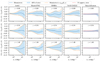 |
Fig. 2. Difference between the symbolic fits for the baryonic effect on the power spectrum (Spred) to the true values (S) from the test set. Each column is for a different baryonic model, and each row is for a different redshift, z. The solid lines indicate the mean difference and the shaded region contains 68% of samples. In the dashed orange lines we show the symbolic fits to the error on our models, as given in Table 4. This error is due to a combination of stochasticity in the simulation and imperfect symbolic approximations. The dashed red line in the baryonification model shows the approximate 1% intrinsic error of the BACCO emulator.
Table 4. Chosen model for the error on baryonic correction to the power spectrum as a function of wavenumber k and redshift z. |
To determine the accuracy of these models, in Fig. 2 we plot the distribution of errors between our symbolic approximations to S and the true values from the test set for a range of redshifts between z = 0 and 1.5. We plot both the mean difference as a function of k as well as the 68% error band. Since we already include a term fit to remove the offset (although this is obtained using the training set), we see that the mean offset is approximately zero for all k, z and model, and is consistent with zero within the 68% error band.
For the baryonification model, the difference between the truth and prediction is strictly an error due to imperfect SR, and has a root mean squared value of 0.7% for both the training and test sets, with increasing error as one increases k. This is the error on the fit to BACCO’s emulation of the baryonification model, which matches the cosmological simulations to within 1–2%. These errors should be combined to estimate the total error.
The hydrodynamical simulations, however, exhibit significant sample variance, and thus this error is a combination of the inherent stochasticity of the simulation and the error in our fit. To account for this, in Fig. B.1 we plot the normalised error on the test set, where we divide the difference between the truth and our prediction by the standard deviation over the CV set. If the CV set’s standard deviation perfectly captured the stochasticity in the simulation and if our model was perfect up to this effect, the edges of the 68% error bands in Fig. B.1 would be horizontal lines at ±1. This is not quite true, with the errors typically between 1.5 and 2 standard deviations, although for small k we do achieve this ideal accuracy. Given the similar accuracy we obtain to Sharma et al. (2025) (who use a flexible Gaussian process to estimate S), we believe that this imperfection is dominated by the inaccuracy of the variance estimates from the CV set.
Given the significant stochasticity in the hydrodynamic models, for a cosmological analysis it is useful to have both a model for the mean behaviour but also this error, so that this theoretical uncertainty can be summed in quadrature with the covariance matrix of the likelihood. As such, we find symbolic approximations for the errors between the truth and predicted model, ε, as a function of k and z. These are given in Table 4, and one can verify that these tend to zero for small k and high z. These values are plotted in Fig. 2, where we see that these fits are able to smooth out the noisy estimates of this ε due to the finite number of simulations used.
One of the advantages of a symbolic emulator is the ability to enforce exact extrapolation behaviour in certain limits. As indicated in Section 3, we wish to have models for which S(k, z, θ) → 1 as k → 0 or as z → ∞. One can verify analytically that, for the prior range given in Tables 1 and 2, all of the models given in Table 3 obey these requirements. To visualise these limits, in Fig. 3 we plot how our symbolic fits behave as a function of k and z as we take these parameters to very large or very small values, where we set the cosmological and hydrodynamical parameters to their fiducial values. One verifies that, indeed, S becomes unity in the appropriate limits, and that this transition happens smoothly, with the magnitude of baryonic effects growing with time on small scales, whereas the largest scales remain relatively unaffected by their presence.
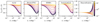 |
Fig. 3. Extrapolation behaviour of our symbolic models for redshifts, z, and wavenumbers, k, outside of the range of the training data. The models are evaluated at the fiducial cosmological and astrophysical parameters (Tables 1 and 2). As is required physically, the correction to the power spectrum, S, becomes unity at high redshift and on large scales (small k). |
Combining these results, in Fig. 4 we plot the true baryonic suppression for four randomly chosen simulations from each of the hydrodynamical simulations, alongside our predictions and error bands. One observes that our symbolic models are able to capture the broad features of this suppression well, despite their different shapes and amplitudes as one varies the cosmological and hydrodynamical parameters. One sees the impact of sample variance, with noisy features in the ‘true’ power spectra, which are smoothed into an estimate of the ensemble mean through our fits, yet whose variance is captured well by ε(k, z).
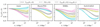 |
Fig. 4. Predicted baryonic suppression of the matter power spectrum, S, as a function of wavenumber, k, at redshift zero for four randomly sampled hydrodynamical simulations at z = 0. Our predictions from Table 3 are shown as solid lines, and the shaded regions give the estimated error on these from Table 4. The dashed lines give the true values measured from the simulations, which are seen to be consistent with our predictions. |
5. Discussion
5.1. Dependence on cosmological and hydrodynamic parameters
One advantage of obtaining analytic expressions for S is that we can now easily interpret the impact of varying individual cosmological and hydrodynamical parameters. In this subsection, we investigate this behaviour, beginning with the impact of cosmology in Section 5.1.1, before turning to hydrodynamics in Section 5.1.2. For the feedback parameters, we find that changing these values can give rise to opposite effects when comparing two hydrodynamical simulations, justifying our approach of conditioning on the model rather than trying to find a single symbolic approximation to fit all these simulations.
With such a comparison, there is a risk that the effects described below are peculiarities of the particular chosen model, rather than an intrinsic property of the hydrodynamic model. To verify this, we show at doi.org/10.5281/zenodo.16754667 that the variation with cosmological and hydrodynamical parameters is similar between multiple OPERON runs per simulation to ensure the robustness of our qualitative conclusions.
5.1.1. Cosmological dependence
The impact of cosmology for the SIMBA and Astrid models is particularly straightforward. For SIMBA, one sees that the only parameters affected by cosmology are  and α2 ∝ Ωm(f(A)+σ8), where f(A) is a function of the hydrodynamic parameters. Hence, one finds that, at large k,
  , and at small k we have
  . Similarly, for the Astrid model,
  , whereas α7 and α8 are linear in Ωm, and α4 is linear in σ8. These combinations mean that the power suppression decreases as Ωm increases for both of these models, which is consistent with Delgado et al. (2023)’s analysis of the SIMBA model. One difference we find with Delgado et al. (2023) is the dependence on σ8; Delgado et al. (2023) suggests that varying σ8 with all other parameters fixed does not drive systematic variations in S, whereas we find that, for both models, increasing σ8 increases the effect of baryons.
The IllustrisTNG model has slightly more complex cosmological behaviour. The σ8 dependence is simple to read off, since α5 is linear in σ8 and thus increasing σ8 increases the effect of baryons. The impact is weaker than varying Ωm, as noted by Delgado et al. (2023), who also studied this model. We see that  and that α2 ∝ Ωm (but α2 is raised to a negative power); hence, the magnitude of the prefactor of the first term in our fit is a decreasing function of Ωm. However, we also have the term
  to consider. For z = 0 this has no effect, and thus we arrive at the same conclusion as Delgado et al. (2023) that increasing Ωm decreases the effect of baryons on the matter power spectrum. Indeed, provided z < 1/(1 − α4)≈1.06, this term cannot result in the opposite trend. For small k, one can ignore the k dependence inside the bracket of the first term of our expression, and thus consider the function 1 + α5α7z. For the fiducial feedback parameters at z ∼ 1, α5α7z ≲ 0.62, and thus this term does not dominate, resulting in the same Ωm behaviour as before. However, for large values of α5 (corresponding to large values of AAGN2/ASN2), one finds that this is no longer true and thus the effect of baryons on the power spectrum can be positively correlated with Ωm provided AGN feedback is much stronger than supernova feedback and at high redshift.
Swift-EAGLE also exhibits a slightly complex dependence on Ωm. Most terms inside the bracket of the first term are proportional to  ; however, α14 also contains a term proportional to
  . The complication arises due to the exponent α1 is raised to, since α1 ∝ Ωm. For very large and small k, this exponent will become larger than 0.625, and is thus guaranteed to lead to a positive correlation between the magnitude of log S and Ωm. However, at z = 0 this only occurs for k < 0.36 h Mpc−1 and k > 37 h Mpc−1, which is outside the range of our training set and thus is an extrapolation effect. Hence, within the range of the training data at z = 0, increasing Ωm decreases the effect of baryons on the power spectrum. At z = 1, some of the small k modes do have the opposite trend, but this effect is negligible given that baryonic suppression is small on these scales.
For all the cosmological simulations, only Ωm and σ8 were varied, so we could not determine the effect of other parameters. However, for the baryonification model we varied many more parameters so we could study their impact. Despite this, we find that many cosmological parameters do not appear in our expressions (h, ns, Mν, w0 and wa), and thus their effect on the baryonic suppression of the power spectrum is minimal (this is also noted by Aricò et al. 2021a). Interestingly, Ωb does appear, since having fixed Ωb is the reason given in Delgado et al. (2023) for the impact of Ωm; as Ωm decreases the baryon fraction of the total matter content increases, making the process of expelling gas out of halos more efficient. Aricò et al. (2021a) also found the dependence on Ωb to be important, in particular in the combination Ωb/Ωm. We see that the effect of baryons within the baryonification model is positively correlated with Ωb, and find the same Ωm dependence as before; for fixed Ωb (and given that 5.823Ωb < 1 for our prior), increasing Ωm decreases the magnitude of log S. σ8 also appears in these expressions with the same trend as before for our prior range.
5.1.2. Dependence on feedback parameters
We now consider the effect of the parameters controlling baryonic physics on the matter power spectrum. Starting with the SIMBA model, we see that both AGN parameters appear linearly in the α2 term of log S, suggesting that increasing either parameter will increase the suppression of power. Moreover, the coefficient of AAGN2 is much larger than for AAGN1; hence, log S is far more sensitive to AAGN2 than AAGN1, as noted by Delgado et al. (2023). The supernova parameters have a rather different effect, where increasing their values reduces the suppression. Again, this is consistent with the findings of Delgado et al. (2023) who interpret this in terms of the non-linear relationship between stellar and AGN feedback; strong stellar feedback suppresses the growth of black holes, weakening the effect of their feedback on matter clustering (Pandey et al. 2023; van Daalen et al. 2011).
If we consider the Astrid model, we see that all of the feedback parameters appear in the parameter α4. AAGN1 appears linearly with a positive coefficient; AAGN2 also appears linearly but with a negative coefficient unless we have particularly weak supernova feedback (ASN2 < 0.56); ASN1 again has a linear dependence but with a negative coefficient across our prior range; and ASN2 appears quadratically, with a coefficient that can take either sign, but is positive for the fiducial parameters. The only other places the feedback parameters appear is in α7 and α8 (which are in the denominator of the first term), where AAGN2 appears linearly with a positive coefficient, and α1 and α3, which are proportional to ASN2. These effects combine to mean that, near the fiducial point, increasing AAGN1 will enhance the suppression of the matter power spectrum, whereas the opposite is true for ASN1 and AAGN2. The impact of ASN2 depends on whether α2k is smaller than 1 or not. This is true for k < 700 h Mpc−1, and thus for all scales of interest. Hence, the AAGN2 parameter has two competing effects: its appearance in α1 and α4 seeks to increase the suppression as it increases, whereas its effect through α3 is to exponentially decrease this suppression. We find that this latter term is the dominant one; thus, increasing AAGN2 decreases the suppression due to baryons.
For the IllustrisTNG model, we find that our expression does not include AAGN1, suggesting that the energy per unit black hole accretion rate for kinetic mode feedback does not significantly affect the matter power spectrum; upon repeating our analysis five times, only two of the six models depend on AAGN1. This is consistent with Delgado et al. (2023) who find little dependence of S on this parameter. The parameter controlling the ejective speed and burstiness of this accretion does affect S, however, with α5 linear in AAGN2, and hence increasing AAGN2 increases the suppression. Similarly, α5 is linear in ASN1 (but with the opposite sign to AAGN2), which leads to a large variation in S as the parameter is varied, where decreasing the feedback strength increases the power suppression, as we saw for the SIMBA model. Although ASN2 appears in two terms of our symbolic approximation (α1 and α5), one can combine these to see that log S is linear in ASN2. The sign of its coefficient is k-dependent, with it equal to zero at k⋆ = 7.5 h Mpc−1 at z = 0 (for all parameters). At higher redshift its value depends on depends on Ωm and the transition occurs at increasingly large scales (smaller k⋆). For k < k⋆, we find that increasing the value of ASN2 decreases the suppression of the matter power spectrum, whereas for larger k the opposite is true. Similar k-dependent effects of the supernova parameters were also discussed in Delgado et al. (2023).
By inspecting the Swift-EAGLE model, we see that increasing any one of AAGN1, AAGN2, or ASN2 will increase the power suppression due to baryons. The dependence on ASN1 is less straightforward, since it appears linearly in α9 (which has the effect of increasing suppression as ASN1 increases); however, it appears in both the numerator and denominator of α10 and α11, so its overall affect on the power spectrum cannot be easily read off, and depends on the values of the other feedback parameters. Setting these to their fiducial values and considering z = 0, we find that the dependence on ASN1 is not monotonic; for k ≲ 5 h Mpc−1, increasing ASN1 initially decreases the amount of baryonic suppression, until we reach very large values (ASN1 ≳ 3), where the suppression increases again. For smaller scales, the impact of ASN1 becomes almost monotonic; however, now increasing ASN1 increases the amount of suppression.
Turning to the baryonification model, we see that almost all the feedback parameters appear in our model, except θout. When fitting this model to various hydrodynamic simulations, Aricò et al. (2021a) note that this parameter is unconstrained, which is consistent with our findings. They also find that the parameters M1 and Minn cannot be inferred from these simulations. Evaluating the expression in Table 3 using the fiducial parameters and z = 0, we find that the term containing α4 is only relevant for k ≲ 10−3 h Mpc−1, whereas the term containing α7 becomes important only after k ≳ 1.5 h Mpc−1. As such, the constraints on any feedback parameters that appear in these terms should be minimal, and indeed M1 and Minn only appear in α4 and α7. Similarly, θinn also only appears in α7, and one observes that there is little variation among the simulations for this parameter. Aricò et al. (2021a) also note that they infer η ≈ 0.5 for all of the simulations considered. We can understand this, since for 10−3 h Mpc−1 ≲ k ≲ 1.5 h Mpc−1, one finds that the baryonification model is proportional to k1 + α6 (provided η < 1). Particularly for the lower end of this k range, one would expect that most of the models should behave similarly, and thus (given α6 only depends on η) it is unsurprising given our fit that all ‘reasonable’ simulations require a similar value of η.
5.2. Small-scale extrapolation behaviour
When obtaining the emulators listed in Table 3, we were limited in terms of the maximum k value we could use. Although we enforced given extrapolation behaviour for large z or low k, the small-scale (high k) extrapolation behaviour was left completely free. In this section we investigate how the models extrapolate as one considers this limit.
Beginning with Astrid, we find that the first term in Table 3 is proportional to kα3 − 1 for large k, whereas the second term is proportional to k. Given the form of α3, we find that the first term is dominant at large k if ASN2 > 2.1, but this is outside the prior range in Table 1. As such, log S ∝ k at large k with a positive coefficient of proportionality, and thus S grows exponentially on small scales.
We find different behaviour for both IllustrisTNG and Swift-EAGLE, for which the first terms are proportional to kγexp(−λk) at large k, where γ = 2 for IllustrisTNG and γ = 1 for Swift-EAGLE. For both cases, λ > 0 and thus at very large k, this term disappears, and the offset term dominates. These both tend to constants at large k, although this constant is independent of z for IllustrisTNG, whereas it grows with z for Swift-EAGLE. These behaviours seem unlikely on physical grounds (one may expect that S would continue to grow on small sclaes) and are thus extrapolation artefacts of the fitting functions. However, when evaluated at the fiducial parameters, the growth with k does not begin to flatten out until k ∼ 50 h Mpc−1 for IllustrisTNG and k ∼ 103 h Mpc−1 for Swift-EAGLE, so for k values far beyond the range of the training data.
The extrapolation properties of SIMBA is a function of redshift. For all z, the first term in Table 3 is proportional to k2 − α4z − α6 with a negative coefficient; hence, at low redshift (z ≲ 0.5) log S → −∞ as k → ∞, and thus S → 0 in this limit. This is surprising given the growth with k seen in Fig. 4; however, we find that the maximum in log S is not reached until k ∼ 103.5 h Mpc−1 for the fiducial parameters, and thus this is an artefact that is not reached until we extrapolate by several orders of magnitude in k. For higher redshift, the first term tends to 0 at high k, and hence we find that S tends to a z-dependent constant at large k.
The baryonification model has a more physical extrapolation behaviour, with log S proportional to k2 + α6 in this regime. α6 is only dependent on the parameter log10(η), and its range in Table 2 means that the exponent is always positive. The sign of the proportionality constant is parameter dependent (and is equal to the negative of the sign of α7), but in all but the most extreme cases it is positive, meaning that S almost always grows as k2 + α6 on small scales, but it can also decay for appropriately chosen parameters.
5.3. Comparison to previous work
Several other works have attempted to find symbolic approximations to baryonic suppression on the matter power spectrum. For example, Gebhardt et al. (2024) use symbolic regression to approximate this quantity for the SIMBA simulation as
 (7)
(7)
where a = {0.25, 0.35, 1.09, 0.14} and 𝒮 is the median normalised gas spread metric, which is a proxy for how far a gas particle is displaced due to the presence of baryonic effects. Other metrics have been used to parametrise the effect of baryons when making such predictions; for example, van Daalen et al. (2020) choose to provide a fitting function for the matter power suppression in terms of the baryonic fraction of massive halos. We note that Gebhardt et al. (2024) use the 1P CAMELS parameter set, which varies one parameter at a time with the others set to their fiducial values, whereas we explore the full prior of Table 1 by using the CV set. Although this model is extremely simple and roughly obeys the correct trends when evaluated on the CV set, the error distribution in Figure 11 of Gebhardt et al. (2024) is significantly larger than those given in Fig. 2; hence, our models are much more accurate. Moreover, Eq. (7) does not obey the correct analytic limit as k → 0, and hence violates the causality constraint on large scales.
An alternative parametrisation that was introduced by Amon & Efstathiou (2022) supposes that the non-linear power spectrum in the presence of baryons, P(k, z), can be expressed in terms of the linear and non-linear dark-matter-only power spectra,  and Pnbody(k, z), respectively. One writes
 (8)
(8)
where Amod is an amplitude parameter that is assumed to be independent of k, z, and background cosmology. Preston et al. (2023) extended this analysis by binning Amod in k bins, such that it can depend on wavenumber, but not redshift or cosmology. The approach is similar in spirit to Bielefeld et al. (2015), who suggest adding extra fitting parameters to non-parametrically fit S(k, z) within a cosmological analysis. Schaller & Schaye (2025) modify this further by assigning an explicit functional form to Amod(k), for which they choose a sigmoid function that depends on three parameters: Alow, kmid, and σmid. Like our fitting functions, this obeys the correct analytic limit as k → 0. However, when fitted against the FLAMINGO simulations (Kugel et al. 2023; Schaye et al. 2023), this sigmoid fit does not produce an upturn in the power spectrum ratio for k ≳ 10 h Mpc−1, but is able to fit the data well before this point. Our models can capture this feature (see, e.g., Fig. 4), which thus represents an advantage of our formulae. Schaller & Schaye (2025) find that Alow and σmid are almost constant across their simulation suite, suggesting that only one parameter is required. Future work could be dedicated to seeing whether this model also fits the CAMELS simulations’ power spectra and how the parameters of this model depend on the varying feedback parameters. Given the success of the fitting formula of Schaller & Schaye (2025), it could be interesting to add additional input features to our models, such as the ratio of the non-linear to linear matter power spectrum, which could help disentangle to effects of baryonic physics and cosmology.
The most similar analysis to our study is that of Sharma et al. (2025), who model S for the same hydrodynamic simulations as in this work; however, they use a Gaussian process rather than symbolic fits. As is described in Section 4, we obtain similar accuracy to Sharma et al. (2025), suggesting that, despite their highly flexible model, the simple formulae given in Table 3 are sufficient for accurately describing this phenomenon.
Schaller et al. (2025) also train a Gaussian process emulator for this task – on the FLAMINGO suite of simulations rather than CAMELS – and are able to obtain high-accuracy predictions of 1% error up to k = 10 h Mpc−1. We have not considered these simulations in this work, but they could represent an ideal target for future SR analyses. Interestingly, they find that S only converges on small scales once the box size is approximately 200 h−1 Mpc per side, which is significantly larger than CAMELS. Although we account for this sample variance using the CV set and obtain models for ε(k, z), this suggests that for a cosmological analysis, one could reduce the magnitude of ε(k, z) in the likelihood, since only the error in the fit (and not the sample variance) should be significant for larger volumes. Not only could one use larger volume simulations to see how our approach performs in such settings, but one could also attempt to train on higher-resolution simulations to assess the robustness as one resolves smaller-scale processes.
One need not parametrise the effect of baryons in terms of the input hydrodynamic and cosmological parameters, but instead use emergent properties of the simulation. For example, the SP(k) emulator of Salcido et al. (2023) is able to reproduce the matter power spectrum accurately from the mean baryon fraction of halos. Similarly, Pandey et al. (2023) also study power suppression in the context of the CAMELS simulations, choosing to use a random forest to predict power suppression from observable quantities. The uncertainties on their model (see Figures 6 and 7 of Pandey et al. 2023) are slightly larger than the estimate from the CV set, justifying our claim in Section 4 that it is not a concern that the normalised errors in Fig. B.1 extend to greater than unity. Pandey et al. (2023) also show in their appendix that, although the N-body power suppression is relatively robust to the choice of box size for the k range we consider, it is somewhat sensitive to the resolution. This again supports our decision to not attempt to try to further reduce the errors from Fig. B.1, since there is an additional systematic error on S that has not been considered here. Delgado et al. (2023) also train a random forest on the CAMELS simulations to make this prediction but as a function of other variables. An extensive comparison of their conclusions to our models is given in Section 5.1.
6. Conclusion
To fully exploit data from current and upcoming cosmological surveys, we must be able to model the non-negligible effects of baryons on the clustering of matter in the Universe. Different hydrodynamical models yield significantly different (and highly stochastic) predictions for the impact of baryons. These simulations are computationally expensive, and hence emulating their behaviour is essential if one wishes to incorporate these within cosmological analysis pipelines.
As such, in this work we used symbolic regression to obtain symbolic approximations for the suppression of the matter power spectrum due to the inclusion of baryons for four implementations of sub-grid physics in hydrodynamical simulations (Astrid, IllustrisTNG, SIMBA and Swift-EAGLE) as well as one baryonification model. This suppression is sufficient for modelling baryonic effects at the field level for scales up to k ∼ 10 h Mpc−1 (Sharma et al. 2025). These expressions are given in Table 3, which summarises the main results of the paper. For the hydrodynamical simulations, our models achieve similar accuracy to previous (non-symbolic) emulators, and we characterise this error – which is comparable to our estimate of sample variance – also in terms of symbolic expressions (Table 4). Our fits for the baryonification model have a root mean squared error of 0.7% compared to the BACCO emulator (Aricò et al. 2021a), although this error increases towards small scales and must be combined with the error on the BACCO emulator itself compared to hydrodynamic simulations (approximately 1–2%).
By construction, our models extrapolate to give the correct physical behaviour on the largest scales and at early times. Since they are symbolic, we are able to easily determine the impact of varying cosmological and hydrodynamical parameters to gain physical insight into how feedback processes affect the clustering of matter. Our models are compact and are comprised of elementary mathematical operations, and are thus trivial to export to programming language of the user’s choice without reliance on external packages (although we make Python implementations publicly available).
We chose to focus on the publicly available CAMELS simulations and one baryonification model; however, future work should be dedicated to applying a similar methodology to a broader range of models, to enable their comparison at the level of the power spectrum (for example, using the power spectrum library of van Daalen et al. 2020). One of the advantages of the baryonification model is its flexibility such that, for appropriate choices of parameters, it can approximate many different hydrodynamic simulations (Aricò et al. 2021a). In future work, it would be interesting to investigate the flexibility of the other models in Table 3 and whether these models are distinguishable when used in cosmological analyses. Alternatively, one could attempt to find a single symbolic expression that is able to model all simulations well and interpolate between hydrodynamic models. For the hydrodynamical simulations, one could also extend the number and range of parameters varied to see what impact other feedback parameters have on the power spectrum. In terms of cosmological parameters, it would be particularly interesting to vary Ωb alongside Ωm and σ8 in the hydrodynamical simulations, since these are the only three cosmological parameters that are important for determining the suppression within the baryonification model studied here. Finally, given the substantial sample variance observed between different CAMELS simulations, it would be useful to investigate how our models behave when applied to larger volume simulations, where this effect should be smaller, for example with the FLAMINGO simulations (Kugel et al. 2023; Schaye et al. 2023). Given the non-linear and non-Gaussian nature of baryonic effects, one could also extend our emulation approach to quantity the effects of baryons on other quantities of interest in cosmology, such as the matter bispectrum.
Our approach has been centred on the idea of conditioning on a particular model (i.e. finding a single symbolic approximation for each model) rather than obtaining a single, flexible model that is robust to the implementation of hydrodynamic physics. This should enable future work to embed these different models within pipelines for inference on real cosmological datasets, and thus one will be able to compute evidence ratios to determine which model is favoured by the data, and inform the development of future subgrid models.
In summary, we have demonstrated that symbolic regression offers a powerful, interpretable, and highly portable method to emulate the impact of baryonic physics on cosmological quantities such as the matter power spectrum. By providing compact analytic forms tailored to specific hydrodynamical and baryonification models, our results bridge the gap between high-fidelity simulations and practical cosmological inference. These symbolic models not only reproduce the known behaviour of baryonic suppression with competitive accuracy but also offer new opportunities for model comparison and parameter exploration with upcoming surveys.
Data availability
We provide Python implementations of the models in Tables 3 and 4 at github.com/DeaglanBartlett/symbolicpofk. The data underlying this article will be shared on reasonable request to the corresponding authors. Parameter dependencies of our models are shown at doi.org/10.5281/zenodo.16754667.
Acknowledgments
We thank David Alonso, Carlos Garcia-Garcia, Francisco Villaescusa-Navarro, Joop Schaye, and Matteo Zennaro for useful comments and suggestions. DJB was supported by the Simons Collaboration on “Learning the Universe” and is supported by Schmidt Sciences through The Eric and Wendy Schmidt AI in Science Fellowship. HD is supported by a Royal Society University Research Fellowship (grant no. 211046). PGF acknowledges support from STFC and the Beecroft Trust.
References
- AbdusSalam, S., Abel, S., & Romão, M. C. 2025, Phys. Rev. D, 111, 015022 [Google Scholar]
- Amon, A., & Efstathiou, G. 2022, MNRAS, 516, 5355 [CrossRef] [Google Scholar]
- Aricò, G., Angulo, R. E., Hernández-Monteagudo, C., et al. 2020, MNRAS, 495, 4800 [Google Scholar]
- Aricò, G., Angulo, R. E., Contreras, S., et al. 2021a, MNRAS, 506, 4070 [CrossRef] [Google Scholar]
- Aricò, G., Angulo, R. E., Hernández-Monteagudo, C., Contreras, S., & Zennaro, M. 2021b, MNRAS, 503, 3596 [Google Scholar]
- Aricò, G., Angulo, R. E., Zennaro, M., et al. 2023, A&A, 678, A109 [NASA ADS] [CrossRef] [EDP Sciences] [Google Scholar]
- Bartlett, D. J., Desmond, H., & Ferreira, P. G. 2023, in The Genetic and Evolutionary Computation Conference 2023 [Google Scholar]
- Bartlett, D. J., Kammerer, L., Kronberger, G., et al. 2024a, A&A, 686, A209 [NASA ADS] [CrossRef] [EDP Sciences] [Google Scholar]
- Bartlett, D. J., Wandelt, B. D., Zennaro, M., Ferreira, P. G., & Desmond, H. 2024b, A&A, 686, A150 [NASA ADS] [CrossRef] [EDP Sciences] [Google Scholar]
- Bassini, L., Rasia, E., Borgani, S., et al. 2020, A&A, 642, A37 [NASA ADS] [CrossRef] [EDP Sciences] [Google Scholar]
- Bielefeld, J., Huterer, D., & Linder, E. V. 2015, JCAP, 2015, 023 [Google Scholar]
- Bigwood, L., Amon, A., Schneider, A., et al. 2024, MNRAS, 534, 655 [NASA ADS] [CrossRef] [Google Scholar]
- Bird, S., Viel, M., & Haehnelt, M. G. 2012, MNRAS, 420, 2551 [Google Scholar]
- Bragança, D. P. L., Lewandowski, M., Sekera, D., Senatore, L., & Sgier, R. 2021, JCAP, 2021, 074 [Google Scholar]
- Burlacu, B. 2023, Proceedings of the Companion Conference on Genetic and Evolutionary Computation, GECCO ’23 Companion (New York, NY, USA: Association for Computing Machinery), 2412 [Google Scholar]
- Burlacu, B., Kronberger, G., & Kommenda, M. 2020, Proceedings of the 2020 Genetic and Evolutionary Computation Conference Companion, GECCO ’20 (New York, NY, USA: Association for Computing Machinery), 1562 [Google Scholar]
- Cava, W. G. L., Orzechowski, P., Burlacu, B., et al. 2021, arXiv e-prints [arXiv:2107.14351] [Google Scholar]
- Chen, A., Aricò, G., Huterer, D., et al. 2023, MNRAS, 518, 5340 [Google Scholar]
- Chisari, N. E., Richardson, M. L. A., Devriendt, J., et al. 2018, MNRAS, 480, 3962 [Google Scholar]
- Crain, R. A., Schaye, J., Bower, R. G., et al. 2015, MNRAS, 450, 1937 [NASA ADS] [CrossRef] [Google Scholar]
- Dai, B., Feng, Y., & Seljak, U. 2018, JCAP, 2018, 009 [Google Scholar]
- Davé, R., Anglés-Alcázar, D., Narayanan, D., et al. 2019, MNRAS, 486, 2827 [Google Scholar]
- Debackere, S. N. B., Schaye, J., & Hoekstra, H. 2020, MNRAS, 492, 2285 [Google Scholar]
- Delgado, A. M., Anglés-Alcázar, D., Thiele, L., et al. 2023, MNRAS, 526, 5306 [Google Scholar]
- Dolag, K., Mevius, E., & Remus, R.-S. 2017, Galaxies, 5, 35 [NASA ADS] [CrossRef] [Google Scholar]
- Dubois, Y., Pichon, C., Welker, C., et al. 2014, MNRAS, 444, 1453 [Google Scholar]
- Eifler, T., Krause, E., Dodelson, S., et al. 2015, MNRAS, 454, 2451 [Google Scholar]
- Fedeli, C. 2014, JCAP, 2014, 028 [CrossRef] [Google Scholar]
- Fedeli, C., Semboloni, E., Velliscig, M., et al. 2014, JCAP, 2014, 028 [Google Scholar]
- Feng, Y., Di-Matteo, T., Croft, R. A., et al. 2016, MNRAS, 455, 2778 [NASA ADS] [CrossRef] [Google Scholar]
- Foreman, S., Becker, M. R., & Wechsler, R. H. 2016, MNRAS, 463, 3326 [NASA ADS] [CrossRef] [Google Scholar]
- García-García, C., Zennaro, M., Aricò, G., Alonso, D., & Angulo, R. E. 2024, JCAP, 08, 024 [Google Scholar]
- Gebhardt, M., Anglés-Alcázar, D., Borrow, J., et al. 2024, MNRAS, 529, 4896 [NASA ADS] [CrossRef] [Google Scholar]
- Giri, S. K., & Schneider, A. 2021, JCAP, 2021, 046 [Google Scholar]
- Hadzhiyska, B., Ferraro, S., Ried Guachalla, B., et al. 2024, arXiv e-prints [arXiv:2407.07152] [Google Scholar]
- Hikage, C., Oguri, M., Hamana, T., et al. 2019, PASJ, 71, 43 [Google Scholar]
- Hopkins, P. F. 2015, MNRAS, 450, 53 [Google Scholar]
- Huang, H.-J., Eifler, T., Mandelbaum, R., & Dodelson, S. 2019, MNRAS, 488, 1652 [NASA ADS] [CrossRef] [Google Scholar]
- Jo, Y., Genel, S., Sengupta, A., et al. 2025, arXiv e-prints [arXiv:2502.13239] [Google Scholar]
- Kodwani, D., Alonso, D., & Ferreira, P. 2019, Open J. Astrophys., 2, 3 [NASA ADS] [CrossRef] [Google Scholar]
- Köhlinger, F., Viola, M., Valkenburg, W., et al. 2016, MNRAS, 456, 1508 [Google Scholar]
- Köhlinger, F., Viola, M., Joachimi, B., et al. 2017, MNRAS, 471, 4412 [Google Scholar]
- Kommenda, M., Burlacu, B., Kronberger, G., & Affenzeller, M. 2020, Genet. Program. Evolvable Mach., 21, 471 [Google Scholar]
- Kronberger, G., Burlacu, B., Kommenda, M., Winkler, S. M., & Affenzeller, M. 2024, Symbolic Regression (Chapman& Hall/CRC Press) [Google Scholar]
- Kugel, R., Schaye, J., Schaller, M., et al. 2023, MNRAS, 526, 6103 [NASA ADS] [CrossRef] [Google Scholar]
- Laumanns, M., Thiele, L., Deb, K., & Zitzler, E. 2002, Evol. Comput., 10, 263 [CrossRef] [Google Scholar]
- Lee, J., Shin, J., Snaith, O. N., et al. 2021, ApJ, 908, 11 [CrossRef] [Google Scholar]
- Levenberg, K. 1944, Q. Appl. Math., 2, 164 [Google Scholar]
- Lewandowski, M., Perko, A., & Senatore, L. 2015, JCAP, 2015, 019 [Google Scholar]
- Lovell, C. C., Starkenburg, T., Ho, M., et al. 2024, arXiv e-prints [arXiv:2411.13960] [Google Scholar]
- Lu, T., & Haiman, Z. 2021, MNRAS, 506, 3406 [NASA ADS] [CrossRef] [Google Scholar]
- Maraio, A., Hall, A., & Taylor, A. 2025, MNRAS, 537, 1749 [Google Scholar]
- Marquardt, D. W. 1963, J. Soc. Indust. Appl. Math., 11, 431 [CrossRef] [Google Scholar]
- Martin-Alvarez, S., Iršic, V., Koudmani, S., et al. 2024, Stirring the cosmic pot: how black hole feedback shapes the matter power spectrum in the Fable simulations (Oxford University Press) [Google Scholar]
- McCarthy, I. G., Schaye, J., Bird, S., & Le Brun, A. M. C. 2017, MNRAS, 465, 2936 [Google Scholar]
- Mead, A. J., Peacock, J. A., Heymans, C., Joudaki, S., & Heavens, A. F. 2015, MNRAS, 454, 1958 [NASA ADS] [CrossRef] [Google Scholar]
- Mead, A. J., Brieden, S., Tröster, T., & Heymans, C. 2021, MNRAS, 502, 1401 [Google Scholar]
- Mohammed, I., Martizzi, D., Teyssier, R., & Amara, A. 2014, arXiv e-prints [arXiv:1410.6826] [Google Scholar]
- Nelson, D., Springel, V., Pillepich, A., et al. 2019, Computat. Astrophys. Cosmol., 6, 2 [NASA ADS] [CrossRef] [Google Scholar]
- Ni, Y., Di Matteo, T., Bird, S., et al. 2022, MNRAS, 513, 670 [NASA ADS] [CrossRef] [Google Scholar]
- Ni, Y., Genel, S., Anglés-Alcázar, D., et al. 2023, ApJ, 959, 136 [NASA ADS] [CrossRef] [Google Scholar]
- Pandey, S., Lehman, K., Baxter, E. J., et al. 2023, MNRAS, 525, 1779 [CrossRef] [Google Scholar]
- Pillepich, A., Springel, V., Nelson, D., et al. 2018, MNRAS, 473, 4077 [Google Scholar]
- Preston, C., Amon, A., & Efstathiou, G. 2023, MNRAS, 525, 5554 [NASA ADS] [CrossRef] [Google Scholar]
- Salcido, J., McCarthy, I. G., Kwan, J., Upadhye, A., & Font, A. S. 2023, MNRAS, 523, 2247 [NASA ADS] [CrossRef] [Google Scholar]
- Schaller, M., & Schaye, J. 2025, MNRAS, 540, 2322 [Google Scholar]
- Schaller, M., Borrow, J., Draper, P. W., et al. 2024, MNRAS, 530, 2378 [NASA ADS] [CrossRef] [Google Scholar]
- Schaller, M., Schaye, J., Kugel, R., Broxterman, J. C., & van Daalen, M. P. 2025, MNRAS, 539, 1337 [Google Scholar]
- Schaye, J., Dalla Vecchia, C., Booth, C. M., et al. 2010, MNRAS, 402, 1536 [Google Scholar]
- Schaye, J., Crain, R. A., Bower, R. G., et al. 2015, MNRAS, 446, 521 [Google Scholar]
- Schaye, J., Kugel, R., Schaller, M., et al. 2023, MNRAS, 526, 4978 [NASA ADS] [CrossRef] [Google Scholar]
- Schneider, A., & Teyssier, R. 2015, JCAP, 2015, 049 [Google Scholar]
- Schneider, A., Teyssier, R., Stadel, J., et al. 2019, JCAP, 2019, 020 [Google Scholar]
- Schneider, A., Refregier, A., Grandis, S., et al. 2020, JCAP, 2020, 020 [CrossRef] [Google Scholar]
- Semboloni, E., Hoekstra, H., Schaye, J., van Daalen, M. P., & McCarthy, I. G. 2011, MNRAS, 417, 2020 [Google Scholar]
- Semboloni, E., Hoekstra, H., & Schaye, J. 2013, MNRAS, 434, 148 [CrossRef] [Google Scholar]
- Shao, H., Villaescusa-Navarro, F., Villanueva-Domingo, P., et al. 2023, ApJ, 944, 27 [Google Scholar]
- Sharma, D., Dai, B., Villaescusa-Navarro, F., & Seljak, U. 2025, MNRAS, 538, 1415 [Google Scholar]
- Somerville, R. S., & Davé, R. 2015, ARA&A, 53, 51 [Google Scholar]
- Springel, V. 2010, MNRAS, 401, 791 [Google Scholar]
- Springel, V., Pakmor, R., Zier, O., & Reinecke, M. 2021, MNRAS, 506, 2871 [NASA ADS] [CrossRef] [Google Scholar]
- Sui, C., Bartlett, D. J., Pandey, S., et al. 2025, A&A, 698, A1 [NASA ADS] [CrossRef] [EDP Sciences] [Google Scholar]
- Sullivan, J. M., Seljak, U., & Singh, S. 2021, JCAP, 2021, 026 [CrossRef] [Google Scholar]
- Terasawa, R., Li, X., Takada, M., et al. 2025, Phys. Rev. D, 111, 063509 [Google Scholar]
- Tröster, T., Ferguson, C., Harnois-Déraps, J., & McCarthy, I. G. 2019, MNRAS, 487, L24 [Google Scholar]
- van Daalen, M. P., Schaye, J., Booth, C. M., & Dalla Vecchia, C. 2011, MNRAS, 415, 3649 [Google Scholar]
- van Daalen, M. P., McCarthy, I. G., & Schaye, J. 2020, MNRAS, 491, 2424 [Google Scholar]
- Villaescusa-Navarro, F. 2018, Pylians: Python libraries for the analysis of numerical simulations, Astrophysics Source Code Library [record ascl:1811.008] [Google Scholar]
- Villaescusa-Navarro, F., Anglés-Alcázar, D., Genel, S., et al. 2021a, ApJ, 915, 71 [NASA ADS] [CrossRef] [Google Scholar]
- Villaescusa-Navarro, F., Genel, S., Angles-Alcazar, D., et al. 2021b, arXiv e-prints [arXiv:2109.10360] [Google Scholar]
- Villaescusa-Navarro, F., Wandelt, B. D., Anglés-Alcázar, D., et al. 2022, ApJ, 928, 44 [NASA ADS] [CrossRef] [Google Scholar]
- Villaescusa-Navarro, F., Genel, S., Anglés-Alcázar, D., et al. 2023, ApJS, 265, 54 [NASA ADS] [CrossRef] [Google Scholar]
- Villanueva-Domingo, P., & Villaescusa-Navarro, F. 2022, ApJ, 937, 115 [NASA ADS] [CrossRef] [Google Scholar]
- Villanueva-Domingo, P., Villaescusa-Navarro, F., Anglés-Alcázar, D., et al. 2022, ApJ, 935, 30 [NASA ADS] [CrossRef] [Google Scholar]
- Vogelsberger, M., Genel, S., Springel, V., et al. 2014, Nature, 509, 177 [Google Scholar]
- Vogelsberger, M., Marinacci, F., Torrey, P., & Puchwein, E. 2020, Nat. Rev. Phys., 2, 42 [Google Scholar]
- Wadekar, D., Thiele, L., Hill, J. C., et al. 2023a, MNRAS, 522, 2628 [NASA ADS] [CrossRef] [Google Scholar]
- Wadekar, D., Thiele, L., Villaescusa-Navarro, F., et al. 2023b, Proc. Nat. Acad. Sci., 120, e2202074120 [NASA ADS] [CrossRef] [Google Scholar]
- Weinberger, R., Springel, V., Hernquist, L., et al. 2017, MNRAS, 465, 3291 [Google Scholar]
- Weinberger, R., Springel, V., & Pakmor, R. 2020, ApJS, 248, 32 [Google Scholar]
- White, M. 2004, Astropart. Phys., 22, 211 [Google Scholar]
- Zhan, H., & Knox, L. 2004, ApJ, 616, L75 [Google Scholar]
Appendix A: Pareto Fronts
In this appendix we plot the Pareto fronts for the models of log S. These are given in Fig. A.1, where we plot the training and test losses (NMSE) against model length. We chose the models indicated by the dashed vertical lines, using the selection criteria outlined in Section 3, and these are given in Table 3.
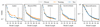 |
Fig. A.1. Pareto front of solutions found with OPERON for log S (Eq. (2)). We plot the training and test sets separately, and the dashed lines indicate our chosen models. |
Appendix B: Comparison of emulator error to sample variance
This appendix compares the accuracy of our symbolic emulators for the hydrodynamical simulations (evaluated on the test set) to the sample variance given by the CV set. The ratios of these two quantities are given in Fig. B.1. If our emulators were perfect and the CV set exactly captured the sample variance, then the bands plotted in Fig. B.1 would be horizontal and span between −1 and 1. This is not quite true, with the bands typically at 1.5 to 2σ. As discussed in Section 4, we expect that this is dominated by the inaccuracies of the sample variance estimation.
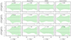 |
Fig. B.1. Same as Fig. 2, but where we divide the difference between the truth and prediction by the standard deviation of the CV set. For a perfect symbolic fit and if this standard deviation perfectly captured the stochasticity, then the shaded region would be a band between -1 and 1. |
All Tables
Range of the cosmological (upper) and hydrodynamical (lower) parameters used in the CAMELS simulations considered.
Ranges of the cosmological (upper) and baryonification (lower) parameters used and their fiducial values.
Chosen model for the error on baryonic correction to the power spectrum as a function of wavenumber k and redshift z.
All Figures
|
Fig. 1. Baryonic effect, log S (Eq. (2)), on the power spectrum for the 27 CV simulations and its standard deviation over k for the Astrid sub-grid model at z = 0. |
| In the text | |
|
Fig. 2. Difference between the symbolic fits for the baryonic effect on the power spectrum (Spred) to the true values (S) from the test set. Each column is for a different baryonic model, and each row is for a different redshift, z. The solid lines indicate the mean difference and the shaded region contains 68% of samples. In the dashed orange lines we show the symbolic fits to the error on our models, as given in Table 4. This error is due to a combination of stochasticity in the simulation and imperfect symbolic approximations. The dashed red line in the baryonification model shows the approximate 1% intrinsic error of the BACCO emulator.
Table 4. Chosen model for the error on baryonic correction to the power spectrum as a function of wavenumber k and redshift z. |
| In the text | |
|
Fig. 3. Extrapolation behaviour of our symbolic models for redshifts, z, and wavenumbers, k, outside of the range of the training data. The models are evaluated at the fiducial cosmological and astrophysical parameters (Tables 1 and 2). As is required physically, the correction to the power spectrum, S, becomes unity at high redshift and on large scales (small k). |
| In the text | |
|
Fig. 4. Predicted baryonic suppression of the matter power spectrum, S, as a function of wavenumber, k, at redshift zero for four randomly sampled hydrodynamical simulations at z = 0. Our predictions from Table 3 are shown as solid lines, and the shaded regions give the estimated error on these from Table 4. The dashed lines give the true values measured from the simulations, which are seen to be consistent with our predictions. |
| In the text | |
|
Fig. A.1. Pareto front of solutions found with OPERON for log S (Eq. (2)). We plot the training and test sets separately, and the dashed lines indicate our chosen models. |
| In the text | |
|
Fig. B.1. Same as Fig. 2, but where we divide the difference between the truth and prediction by the standard deviation of the CV set. For a perfect symbolic fit and if this standard deviation perfectly captured the stochasticity, then the shaded region would be a band between -1 and 1. |
| In the text | |
Current usage metrics show cumulative count of Article Views (full-text article views including HTML views, PDF and ePub downloads, according to the available data) and Abstracts Views on Vision4Press platform.
Data correspond to usage on the plateform after 2015. The current usage metrics is available 48-96 hours after online publication and is updated daily on week days.
Initial download of the metrics may take a while.