| Issue |
A&A
Volume 702, October 2025
ZTF SN Ia DR2
|
|
|---|---|---|
| Article Number | A190 | |
| Number of page(s) | 13 | |
| Section | Extragalactic astronomy | |
| DOI | https://doi.org/10.1051/0004-6361/202450392 | |
| Published online | 24 October 2025 | |
ZTF SN Ia DR2: Cosmology-independent constraints on Type Ia supernova standardisation from supernova siblings
1
Institute of Astronomy and Kavli Institute for Cosmology, University of Cambridge, Madingley Road, Cambridge CB3 0HA, UK
2
The Oskar Klein Centre for Cosmoparticle Physics, Department of Physics, Stockholm University, SE-10691 Stockholm, Sweden
3
Université de Lyon, Université Claude Bernard Lyon 1, CNRS/IN2P3, IP2I Lyon, F-69622 Villeurbanne, France
4
Department of Physics, Lancaster University, Lancs LA1 4YB, UK
5
School of Physics, Trinity College Dublin, The University of Dublin, Dublin 2, Ireland
6
Institut für Physik, Humboldt-Universität zu Berlin, Newtonstr. 15, 12489 Berlin, Germany
7
Lawrence Berkeley National Laboratory, 1 Cyclotron Road MS 50B-4206, Berkeley CA 94720, USA
8
Department of Astronomy, University of California, Berkeley, 501 Campbell Hall, Berkeley CA 94720, USA
9
Institute of Space Sciences (ICE, CSIC), Campus UAB, Carrer de Can Magrans, s/n, E-08193 Barcelona, Spain
10
Institut d’Estudis Espacials de Catalunya (IEEC), E-08034 Barcelona, Spain
11
The Oskar Klein Centre, Department of Astronomy, Stockholm University, Albanova University Center, Stockholm SE-106 91, Sweden
12
LPNHE, (CNRS/IN2P3, Sorbonne Université, Université Paris Cité), Laboratoire de Physique Nucléaire et de Hautes Énergies, 75005 Paris, France
13
Nordic Optical Telescope, Rambla José Ana Fernández Pérez 7 ES-38711 Breña Baja, Spain
14
Université Clermont Auvergne, CNRS/IN2P3, LPCA, F-63000 Clermont-Ferrand, France
15
IPAC, California Institute of Technology, Pasadena CA 91125, USA
16
Caltech Optical Observatories, California Institute of Technology, Pasadena CA 91125, USA
17
School of Physics and Astronomy, University of Minnesota Minneapolis MN 55455, USA
⋆ Corresponding author: This email address is being protected from spambots. You need JavaScript enabled to view it.
Received:
15
April
2024
Accepted:
26
March
2025
Abstract
Understanding Type Ia supernovae (SNe Ia) and the empirical standardisation relations that make them excellent distance indicators is vital to improving cosmological constraints. SN Ia ‘siblings, i.e. two or more SNe Ia in the same host or parent galaxy, offer a unique way to infer the standardisation relations and their scatter across the population. We analysed a sample of 25 SN Ia pairs observed homogeneously by the Zwicky Transient Facility (ZTF) to infer the SNe Ia light curve width-luminosity and colour-luminosity parameters, α and β. Using the pairwise constraints from siblings, which allow for a scatter in the standardisation relations, we found α = 0.218 ± 0.055 and β = 3.084 ± 0.312, respectively, with a dispersion in α and β of ≤0.195 and ≤0.923, respectively, at a 95% confidence level. While the median dispersion is large, the values within ∼1σ are consistent with no dispersion. Hence, fitting for a single global standardisation relation, we found α = 0.228 ± 0.029 and β = 3.160 ± 0.191. We also found a very small intrinsic scatter of the siblings sample σint ≤ 0.10 mag at a 95% confidence level compared to σint = 0.22 ± 0.04 mag when computing the scatter using the Hubble residuals without comparing them as siblings. When comparing to large samples used in cosmological measurements, we found an α that is ∼2-3 σ higher, while the β values are consistent. The high α is driven by low x1 pairs, potentially suggesting that the slow and fast declining SN Ia have different slopes for the width-luminosity relation. We found no difference in α and β when dividing the sample by host galaxy mass. The finding of a higher α with increased statistics can be confirmed or refuted through upcoming time-domain surveys. If confirmed, this finding can improve the cosmological inference from SNe Ia and be used to infer properties of the progenitors for subpopulations of SNe Ia.
Key words: supernovae: general / cosmological parameters / dark energy / distance scale / large-scale structure of Universe
© The Authors 2025
 Open Access article, published by EDP Sciences, under the terms of the Creative Commons Attribution License (https://creativecommons.org/licenses/by/4.0), which permits unrestricted use, distribution, and reproduction in any medium, provided the original work is properly cited.
This article is published in open access under the Subscribe to Open model. This email address is being protected from spambots. You need JavaScript enabled to view it. to support open access publication.
1. Introduction
Type Ia supernovae (SNe Ia) are excellent distance indicators in cosmology, and they are instrumental to the discovery of the accelerated expansion of the Universe (Riess et al. 1998; Perlmutter et al. 1999). SNe Ia are also crucial to precisely measuring dark energy and the Hubble constant (e.g. DES Collaboration 2024; Rubin et al. 2023; Brout et al. 2022a; Riess et al. 2022). In optical wavelengths, which is the regime where most constraints on cosmology from SNe Ia are obtained, standardisation of the SN Ia peak luminosity can reduce the scatter to ∼15%. The peak brightness is corrected for correlations with the light curve width and colour (e.g., Phillips 1993; Tripp 1998) and host galaxy properties (e.g., Kelly et al. 2010; Sullivan et al. 2010). The dependence of width- and colour-corrected luminosity on host galaxy stellar mass, commonly termed the ‘mass step’ is crucial for improving cosmological constraints. The origin of the mass step is poorly understood, but recent studies (e.g. Brout & Scolnic 2021) suggest this could be due to dust and/or intrinsic differences related to astrophysical properties, such as progenitor age (Rigault et al. 2020; Briday et al. 2022). As SN Ia cosmology is currently systematics limited, understanding the standardisation relations is crucial to constraining their cosmology. This is particularly important since several future Stage-IV dark energy missions are designed with a sizable component devoted to a high-redshift SN Ia survey (Hounsell et al. 2018; The LSST Dark Energy Science Collaboration 2018). At low redshift, a large sample of well-characterised SNe Ia has already been obtained by surveys such as the Zwicky Transient Facility (ZTF; Graham et al. 2019; Bellm et al. 2019; Dekany et al. 2020).
Type Ia supernovae siblings, i.e. multiple SNe Ia in the same parent galaxy (Brown 2015), are a powerful route to constraining the standardisation relations we have mentioned. Recently, SN Ia cosmological samples have been analysed using the SALT2 model (Guy et al. 2007, 2010), wherein the distance modulus μ is obtained by correcting the inferred apparent peak magnitude (mB) for the light curve width (x1) and colour (c) by the relation
 (1)
(1)
where α and β are derived from a simultaneous fit along with cosmology to minimize the scatter in the Hubble-Lemaitre diagram. In the SALT2 formalism, c is an observed colour, which can be viewed as a combination of the intrinsic colour and dust.
The parameter β, which is central to this work, is empirically derived and captures both the intrinsic and extrinsic colour-luminosity relations. In terms of the latter, β can be viewed as an analogue of the total-to-selective absorption ratio in the B-band, RB, for a given dust law (Cardelli et al. 1989). A simultaneous cosmology fit using the largest compiled sample of SNe Ia inferred β = 3.04 ± 0.04 (Brout et al. 2022a), which is significantly lower than the RB ∼ 4.1 seen in the Milky Way (MW; Cardelli et al. 1989; Fitzpatrick 1999). However, other analyses, such as the Union3 compilation (Rubin et al. 2023), have found a higher β compatible with the MW. In cosmological surveys of SNe Ia, it has been noticed that selection effects can lead to incompleteness in the distribution of SNe Ia properties due to correlations with the intrinsic dispersion. These effects will impact the standardisation relations, and they are corrected for using simulations (e.g., Kessler et al. 2019; Popovic et al. 2023). These simulations require detailed inputs of survey observations and the population models derived from the data (e.g. Scolnic & Kessler 2016). Studies exploring the colours of nearby SNe Ia (e,g, Nobili & Goobar 2008) and further expanding the wavelength coverage of the observations from UV to the near-IR (NIR; Burns et al. 2014; Amanullah et al. 2015) indicate a wide range of dust distributions in the interstellar medium (ISM) of SN Ia host galaxies to explain the observed colours. The procedure for the cosmological inference of α and β is convolved with effects such as K-corrections, selection effects, redshift uncertainties, and even MW extinction errors. It is, therefore, important to have independent methods for measuring the standardisation relations. Studies with cosmological samples have shown the likelihood of β values to be dependent on the host galaxy environment (Gonzá lez-Gaitán et al. 2021; Brout & Scolnic 2021), which is crucial for making an inference of cosmology based on current and future samples (e.g. see, Dhawan et al. 2024).
Owing to multiple SNe Ia exploding in the same galaxy, the inference obtained from sibling SNe Ia is insensitive to certain systematics, including cosmological model parameters, peculiar velocity corrections, and global host galaxy dependence. Therefore, it is a robust, independent test of the width-luminosity and colour-luminosity relations, as was demonstrated when constraining the colour-luminosity relation (β) from a single sibling pair in Biswas et al. (2022), where β is 3.5 ± 0.3. In the recent literature, it has been posited that SN Ia siblings could have a smaller dispersion in their luminosity compared to SNe Ia in different galaxies (Burns et al. 2020). This is also seen in the small distance dispersion for the three spectroscopically normal SNe Ia in NGC 1316 (Stritzinger et al. 2010), although the spectroscopically peculiar SN 2006mr has a distance modulus that differs by 0.6 mag from that of the other three. Other studies, however, have found no difference between the scatter in SN Ia siblings and non-sibling SNe Ia (Scolnic et al. 2020, 2022). Apart from understanding and improving the distance measurements for cosmology, comparing siblings also has interesting implications for SN Ia physics. Gall et al. (2018) analysed SN2007on and SN2011iv and found a difference of 14% and 9% in their distances from the optical and NIR, respectively. This was attributed to the differences in the progenitor systems, which are hypothesised to be due to different central densities of the primary white dwarf (e.g. Ashall et al. 2018). It is therefore interesting to study SN Ia siblings to both understand the luminosity corrections and test whether the absence of potential systematics in common can increase the precision of distance measurements. While we can collect a large sample of historical SN Ia sibling data (e.g. Anderson & Soto 2013; Kelsey 2023), as mentioned above, it is necessary to have sibling pairs observed on the same system to avoid systematic errors.
In this paper, we analyse a sample of SN Ia siblings homogeneously observed by ZTF. A large part of the sample of SN Ia siblings is derived from the second data release of SNe Ia observed by ZTF (ZTF DR2). We inferred the SALT2 parameters and subsequently the width-luminosity and colour-luminosity relations as presented in equation (1). With a sizable sample of siblings, we present both a cosmology-independent inference of α and β and an estimate of the observed scatter of the two parameters across the sample. Since all SNe Ia are on the same photometric system, the cross-calibration systematics are minimised, which have been a significant source of errors in cosmological studies (e.g. Scolnic et al. 2022; Brout et al. 2022b). We used the ZTF sample of SN Ia siblings to infer SN light curve parameters and simultaneously constrain the width-luminosity and colour-luminosity relations. We present the method we used in Section 2 and the results in Section 3, and we discuss our findings with respect to the literature, specifically, the cosmological sample of SNe Ia, in Section 4. Finally, we conclude in Section 5.
2. Data and methodology
Initial studies of multiple SNe in the same galaxy often focussed on a single pair or a small set of siblings (Hamuy et al. 1991; Stritzinger et al. 2010). With modern time-domain astronomy surveys having a long survey duration, it has been possible to assemble larger samples of SN Ia siblings (Scolnic et al. 2020, 2022; Burns et al. 2020). The first phase of ZTF (ZTF-I) comprises an optical imaging survey of the entire northern sky with a three-day cadence in the g- and r-bands and a ∼20.5 mag depth that operated between 2018 and 2020. It has been augmented to a two-day cadence since 2020 with its successor ZTF-II. This public g- + r-band survey is complemented with partnership surveys in the i-band and higher cadence observations. The unprecedented scanning speed and depth has made ZTF the ideal facility for discovering and characterising SN siblings (Biswas et al. 2022; Graham et al. 2022). Light curves for the objects in this paper were built using a variant on the standard IPAC forced photometry pipeline (Masci et al. 2019), with more details in associated papers (e.g. Smith et al. in prep.).
We constructed our sibling sample by starting with the sample of spectroscopically confirmed ZTF SNe Ia. We queried all transients classified as SNe Ia using fritz (van der Walt et al. 2019; Coughlin et al. 2023) within a 100 arcsecond radius from the SN Ia coordinates (at z ∼ 0.1, this corresponds to a physical separation of ∼35 kpc). We then saved the sample of pairs for which the second object is also associated with the same host galaxy. From this sample, we removed objects that showed continuous variability for more than 60 days before the date of maximum brightness in order to remove persistent transient sources such as active galactic nuclei (AGNs) and tidal disruption events (TDEs). Details of which sibling pairs passed the sample selection are presented in Section A.
For our analyses, we took a sample of 24 sibling pairs where both objects were spectroscopically classified as SN Ia (hereafter, spec) and a sample of 28 pairs with one object spectroscopically classified as SN Ia and one object photometrically classified as SN Ia (hereafter, photo-spec) that have multi-band light curves from ZTF. Below, we describe the process of determining the objects in the photo-spec sample without a classification as SNe Ia1. While we do have two subsamples, we homogeneously analysed the entire sample with the same assumptions and selection cuts. However, for our analysis, we also made consistency checks between the spec and photo-spec subsamples and provided joint constraints. Most of the sibling pairs analysed in this work have at least one member in DR2 of ZTF SNe Ia ((Rigault et al. 2025) hereafter R24; Smith et al. in prep., hereafter S24), and a large fraction of them were classified with the Spectral Energy Distribution Machine (SEDM) on the Palomar 60-inch telescope (Blagorodnova et al. 2018; Rigault et al. 2019). We note that given the approximate rate of one SN Ia per galaxy per century, the total number of sibling pairs in our sample is consistent given the size of the entire DR2 sample is ∼3000 SNe Ia. Since previous studies with SN Ia siblings (e.g., Burns et al. 2020) suggest that cross-calibration systematics are a large error source in sibling analyses, we only constructed our sample from sibling pairs where both SNe are observed by ZTF. Our sample of siblings spans a large redshift range of 0.01 < z < 0.1, as shown in Figure 3.
Currently, the most widely used light curve fitting algorithm is the spectral adaptive light curve template SALT2 (Guy et al. 2010), which is based on the SALT method (Guy et al. 2005), and we used this algorithm in our analysis. The SALT2 model treats the colour entirely empirically and is used to find a global colour-luminosity relation, in contrast to models that distinguish between the intrinsic and dust components (e.g. SNooPy Burns et al. (2011), BayeSN (Mandel et al. 2022; Thorp et al. 2021)). We used the updated version of SALT2 presented in Taylor et al. (2021) and as implemented in sncosmo v2.1.02 (Barbary et al. 2016). We applied the model iteratively. In the first iteration, the fit is without the model covariance, and it is only used to guess the time of maximum. The second iteration fits the model only to the data between −10 and +40 days from the first guess time of maximum (see Rigault et al. in prep. for details on selection of the phase range) and with the model covariance to get all the SALT2 fit parameters simultaneously. In the fitting procedure, we corrected the SN fluxes for extinction due to the dust in the MW using extinction values derived in Schlafly & Finkbeiner (2011). We used the widely applied Galactic reddening law, proposed in Cardelli et al. (1989) and known as the ‘CCM’ law, to correct for MW extinction, with the canonical value for the total-to-selective absorption, RV = RB − 1 = 3.1. We also compared the inferred parameters with those from an older, more widely used version of SALT2 from Betoule et al. (2014), and we found consistent estimates of the inferred parameters. For the SNe in the sample without a spectroscopic classification, we fit template spectral energy distributions for SN Ib/c, IIn, and IIP, as provided very kindly by Peter Nugent3. Only the pairs where the SN without a spectroscopic classification also prefers a fit to an SN Ia template (by a Δχ2 of at least five, though in most cases the fit is overwhelmingly prefers an SN Ia by a Δχ2 of ∼50 or greater) are kept in the sample (Figs. 1 and 2).
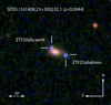 |
Fig. 1. Zwicky Transient Facility RGB image of an example sibling pair from our sample: ZTF20abatows and ZTF20abcawtk. The crosses mark the position of the SNe Ia in the field. These siblings were closest in the time separation (∼5 days between peak for the two SNe) between their peaks and hence were detectable at the same time. |
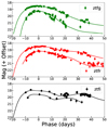 |
Fig. 2. Light curves in the ZTF g, r, i filters along with the SALT2 fits overplotted for the SN Ia pair from the spec subsample with the largest difference in x1, i.e. ZTF18abdmgab and ZTF20abqefja. As discussed in the text, the high Δx1 and low Δc are important for constraining the width-luminosity relation. The difference in x1 in the light curve shapes of the two SNe Ia can be seen as well as the time of the second maximum in the i-band and the r-band shoulder. |
In this work, our aim is to infer the standardisation relations between the SN Ia luminosity and the light curve width and colour. The SALT2 model is typically used with a standardisation relation as parametrised in Tripp (1998):
 (2)
(2)
where the δhost term corresponds to a ‘step-like’ correction either in global or local host galaxy properties, such as stellar mass and star formation rate (e.g. Briday et al. 2022; Scolnic et al. 2022). If the properties in consideration are global (e.g. MW extinction or peculiar velocity correction), then for SN siblings they would ‘l-out’ when inferring the standardisation relations since both SNe in each pair are in the same host galaxy. However, we note that several studies in the literature find a dependence of the SN Ia luminosity on local environmental properties, which would not cancel out in our analysis (Rigault et al. 2015; Roman et al. 2018; Rigault et al. 2020; Kelsey et al. 2021). We fit for α and β using the derived SALT2 parameters (instead of directly at the light curve level) since no degeneracy between α, β, and the SALT2 parameters has been observed (e.g., see Biswas et al. 2022). We note that no explicit K- or S-corrections are mentioned, as the SALT2 model is a spectral template, and hence, these corrections are taken into account when inferring the light curve parameters mB, x1, and c.
In our analyses, we used the Bayes theorem to get the posterior distributions on the parameters of interest, which are α, β, σint, and the spread in α and β. We fit for the α and β values, marginalising over the true x1 and c values. If the observed stretch and colour differences are Δx1o, Δco, the true values can be written as Δx1 = Δx1o + δx1, Δc = Δco + δc, where δx1 and δc are the deviations from the true differences. The difference in the observed distance modulus, for example, due to intrinsic differences in the SN siblings, is given by
 (3)
(3)
 (4)
(4)
The uncertainty of Δμo, that is σΔμo, includes the uncertainties in the observed magnitudes, σmBi2, derived from the output covariance matrix of the SALT2 model fit; the intrinsic magnitude dispersion, σint2; and possible dispersions in the sample of α and β, σα, σβ:
 (5)
(5)
For our analysis, we marginalised over the true values of x1 and c, resulting in χ2 and the following likelihood expression (see Section B for the derivation):
![Mathematical equation: $$ \begin{aligned} \chi ^2 = -2\ln (L) = \sum a - \frac{b^2(c_\alpha + c_\beta )}{(c_m c_\alpha + c_m c_\beta + c_\alpha c_\beta )} + \nonumber \\ \ln \left[\frac{2\pi (c_m c_\alpha + c_m c_\beta + c_\alpha c_\beta )}{c_m c_\alpha c_\beta }\right], \end{aligned} $$](/articles/aa/full_html/2025/10/aa50392-24/aa50392-24-eq6.gif) (6)
(6)
where
 (7)
(7)
 (8)
(8)
 (9)
(9)
 (10)
(10)
 (11)
(11)
SALT2 fit parameters of the SN Ia-SN Ia pairs in this study for the spec and photo-spec subsamples. Details for the light curves and redshifts are provided in Smith et al. in prep.
In our inference, we fit α, β, and their dispersions as free parameters with uniform priors 0 < α < 1, 0 < β < 8, 0 < σ(α) < 5, 0 < σ(β) < 5, and 0 < σint < 2 mag. For the default analysis, we fit with five free parameters, including the intrinsic scatter. In alternate analysis cases, such as where the sample is fitted with a single α and β, we set σα, β = 0. We used PyMultiNest (Buchner et al. 2014), a python wrapper to MultiNest (Feroz et al. 2009), to derive the posterior distribution on the parameters. We used the optimal efficiency of the sampling for parameter inference and 1200 live points, i.e. points drawn uniformly from the prior for sampling. We used a tolerance of 0.05 in the error on the evidence as a criterion for the convergence.
3. Results
In this section, we present SN Ia light curve fit parameters and the inferred value of the luminosity-colour and luminosity-light curve width standardisation relations. We fit the SALT2 model to the light curves for our sample. To create the final sample used for computing the standardisation relations, we removed all objects that had an error on time of maximum σ(t0) > 2 days and observations only in a single filter. Furthermore, we removed objects that lacked adequate sampling at early phases. To quantify this selection criterion, we used the best-sampled SNe, ZTF20acpmgdz and ZTF20achyvas, to perform a test of recovering the SALT2 parameters by downsampling the data and fitting in the absence of early time data. We found that for cases with data at least three days before maximum, we can recover the x1 and c values from the full light curve; however, if the first observation is at a later epoch, the values are biased by > 2σ compared to the inference from the full light curve. We therefore only selected pairs where both SNe have at least one observation three days before to avoid any biases in the α and β measurements from biased x1 and c inference. This left us with 12 spec and 13 photo-spec SN Ia pairs, making a total of 25 pairs.
The parameter distributions are shown in Figure 3 and reported in Table 1. The sibling pairs with the same ZTF name have an extremely small spatial separation but are separated in time. Since the aim is to constrain α and β and not cosmological parameters, we did not make selection cuts on the value of x1 and c in order to allow for the full range of observed light curve widths and colours in our sample. For comparison, in Figure 3, we plot the complete parameter distribution of the ZTF DR2 sample as dashed lines (S24, R24). While the siblings do not extended to the highest redshifts in the DR2 distribution, they span the observed range of x1 and c values of the entire DR2 sample. We note that for direct comparison, we plot the DR2 sample without the cosmological cuts on x1 and c. While the c distribution has a high p-value (0.11) for a Kolmogorov-Smirnov test between the DR2 and the sibling samples, the x1 distribution has a low p-value (0.014), suggesting that even though the siblings span the entire range of observed x1 values in the DR2 sample, the distribution is not drawn from the same parent population. We note from Figure 3 that the mass distribution for the siblings is skewed towards higher values compared to the values for the DR2 distribution. This would be expected for a sibling sample since it is more likely that larger galaxies produce two SNe Ia. This may suggest that since more massive older galaxies typically host low x1 events, we see on average more siblings that have a lower x1 (Rigault et al. 2020; Nicolas et al. 2021).
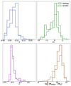 |
Fig. 3. Parameters for the sibling SNe Ia in this study. The panels show the redshift (top left), SALT2 x1 (top right), c (bottom left), and host galaxy stellar mass (bottom right) distributions. We did not make any selection cuts on the values of z, x1, and c, unlike for the complete DR2 sample (Rigault et al. 2025). The equivalent distribution for the entire DR2 sample is overplotted as dashed lines Smith et al. in prep. |
From Figure 4, we found that the difference in the peak magnitude is correlated more significantly with the difference in colour than the light curve width (the Pearson correlation coefficient is r = 0.42 compared to r = −0.045). Therefore, we expected stronger constraints on the β parameter; however, for our fiducial fit, we simultaneously inferred α and β.
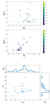 |
Fig. 4. Difference in the inferred SALT2 mB versus the difference in the inferred x1 (top) and c (middle) for each sibling pair in the sample. The siblings with large differences in x1 (and similar values of c) predominantly constrain α precisely, whereas those with a large Δc constrain β. The colour bar shows the x1 for the wider SN (i.e. higher x1; top) and c for the redder (i.e. higher c; middle) SN Ia in the pair. For better visualisation, we plot the Δx1 versus the Δc in the bottom panel. |
The sample has a wide distribution of angular separations for the siblings pairs. In both the spec and phot-spec samples, there are three sibling pairs where the separation is smaller than the pixel size of the camera, and hence, these are ‘same pixel’ siblings (similar to the pair presented in Biswas et al. 2022). This is interesting since the small separation would also indicate that the difference in the properties of the local environment of the SN is small.
We also fit with the dispersion in α and β to account for the scatter in the standardisation relation across the population. This is parameterised by two terms, σ(α) and σ(β), which multiply the Δx1 and Δc terms and are added to the σm. In this formalism, we obtained α = 0.218 ± 0.055 and σ(α)≤0.195 and β = 3.084 ± 0.312 and σ(β)≤0.923, where σα, β are the dispersions in α and β. Below, we evaluate the constraints on the standardisation relations and their dispersion for the individual subsamples, spec and phot-spec, respectively. The constraints on the standardisation parameters are summarised in Table 2 When combining all the pairs to constrain α and β under the assumption of a single α and β, i.e. with the dispersion set to zero, we obtained α = 0.228 ± 0.030 and 3.162 ± 0.191 (Figure 5, black contours).
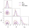 |
Fig. 5. Constraints on α, β, and the intrinsic dispersion (σint) for the complete (black), spectroscopic (violet), and photometric (brown)samples. |
Mean α and β along with the dispersion in both parameters for the complete, spectroscopic only, and photo-spec sample.
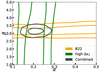 |
Fig. 6. Constraints on α and β from two sibling pairs. The β constraints are from the pair analysed in Biswas et al. (2022) (high Δc, low Δx1), and the α constraints are from the pair ZTF18abdmgab-ZTF20abqefja (high Δx1, low Δc). The figure illustrates the orthogonality in the constraints from high Δc (low Δx1) and high Δx1 (low Δc) sibling pairs. We chose this as a specific case to illustrate that a single pair will have a degeneracy in the α-β plane. However, this degeneracy can be broken by combining the constraints on α-β with constraints from a siblings pair that has orthogonal degeneracy in the two parameter plane. The combined constraints in black are for illustrative purposes; the final constraints on α and β from the combined sample are more stringent than presented here. |
3.1. Spectroscopic SN Ia sample
The SALT2 fit parameters for the spec sample are summarised in Table 1. Unlike the complete ZTF DR2 sample (R24), we did not make selection cuts on the measured value of x1 and c. This is because the objects with x1 and c values outside the range of cosmological values allow for the possibility of a large Δx1 and/or a large Δc, which is important for constraining α and β, respectively. Therefore, the sample has a greater range of observed properties than the complete DR2 sample. The diversity of the entire SN Ia sample from ZTF DR2 is discussed in a companion paper (Dimitriadis et al. 2025). The range of x1 and c parameters provides a long baseline to fit for the standardisation parameters. For one of the pairs with high Δc (i.e. a difference > 0.1), ZTF20acehyxd+ZTF21abouuow, the colour excess attributed to extinction from MW dust (E(B − V)MW) is also significant, i.e. 0.463 mag. We therefore tested the assumption of the MW RV on the inferred β constraint from this SN Ia pair. We varied the MW RV to the line of sight from 2.5 to 3.5 and found no significant shift in the inferred β value. Hence, for our analysis, we continued to adopt the fiducial MW RV = 3.1.
Since our aim is to infer both the standardisation parameters and their dispersion in the sample, we fit the entire spec sample together with the likelihood expressed in equation (6). We found a value of α = 0.217 ± 0.061 and β = 3.084 ± 0.740. This would suggest a mean RV ∼ 2.08 for the sample. Both the α and β dispersion have a high median, though it is consistent within 1σ with no dispersion.
We note that, as expected, the constraints on α are driven by the sibling pairs that have a high Δx1 (and similar c) and the constraints on β by pairs that have a high Δc (and similar x1). The similarity in the c values and large differences in x1 allowed us to break the degeneracy between the α and β constraints since if Δx1 and Δc were otherwise both large, there would be a strong correlation between the inferred α and β.
3.2. Photometric-spectroscopic SN Ia pairs subsample
Along with the sibling pairs of spectroscopically confirmed SNe Ia analysed in Section 3.1, ZTF has also discovered several pairs of SNe in the same galaxy where one SN in the pair is a spectroscopically confirmed SN Ia and the other is a likely SN Ia based on its light curve. We fit the photo-spec pairs with the same method as the spec pairs and report the SALT2 fit parameters values in Table 1. Similar to the spec sample in Section 3.1, we inferred α, β, and the dispersion. We found α = 0.186 ± 0.091 and β = 3.031 ± 0.501. Similar to the spectroscopic subsample, the median dispersion value is high. However, it is consistent with zero at 1σ. The constraints are shown as brown contours in Figure 5. We found that the parameter inference for the phot-spec sample is consistent with the spec sample, and hence, we could combine the samples to get the most precise constraints on α, β, and the dispersion.
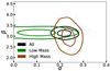 |
Fig. 7. Constraints on α and β from sibling pairs in low (green) and high (brown) mass host galaxies split at the median log10(M*) = 10.57. The values are consistent at 1.5σ between the subsamples. For comparison, the constraints from the entire sample are plotted as well (black). |
3.3. Host galaxy mass dependence
Recent studies have demonstrated that the reddening relations possibly depend on the properties of the host galaxy (e.g. Brout & Scolnic 2021; Gonzá lez-Gaitán et al. 2021). Here, we test whether there is a dependence of the inferred α and β and their dispersions on the host galaxy properties of the sibling pair. From the above results, we found that the spec and photo-spec samples yield consistent values. Therefore, we combined both subsamples for this analysis to gain more statistical precision.
We computed the stellar masses from the g − i colour and i-band absolute magnitude of the host galaxy using the relation provided in Taylor et al. (2011) given as
 (12)
(12)
where mg and mi are MW-extinction corrected apparent magnitudes in the g- and i-bands and Mi is the absolute i-bandmagnitude.
To analyse the dependence, we split the sample into high and low host mass pairs, similar to analyses in the literature with Hubble residuals (e.g. Brout et al. 2022a; Johansson et al. 2021, and references therein). By dividing the sample into low and high mass bins at log(M*/M⊙) = 10, we found consistent results between the two subsamples. However, the statistics in the low mass bin are significantly smaller than for the high mass bin. We therefore split the combined sample at log10(M*/M⊙) = 10.57 and found that the α and β values are consistent at 1.5σ.
3.4. Splitting α based on x1
We tested the sibling sample for evidence of a difference in α between subsamples based on x1. We divided the sample based on the x1 of each SN Ia in a sibling pair to constrain αlow and αhigh, i.e. a single pair can be fitted with a different α if the x1 values for the individual SNe are on different sides of the break. In the literature, a broken stretch-luminosity relation fit has been used in the context of cosmological inference with SNe Ia for low-z and high-z samples (Scolnic et al. 2014; Rubin et al. 2015; Burns et al. 2018). We chose a break value of x1 = −0.49 based on the analysis of the standardisation of the entire ZTF DR2 sample of SNe Ia in (Ginolin et al. 2025). Fitting this broken brightness-stretch relation, the low x1 subsample has an αlow = 0.274 ± 0.045 and αhigh = 0.133 ± 0.072. We perturbed the break value ranging from −1 to 0, including the median value of −0.27, and we found no significant differences in the inferred α values. We surmise that such a difference could arise due to strong selection effects at high z and intrinsic differences in the progenitor population.
4. Discussion
We constrained the standardisation relations of SNe Ia with the spec and photo-spec subsamples and a joint analysis with all the sibling pairs. Accurately constraining the standardisation relations is key to improving cosmological constraints with current and future SN Ia datasets (Brout et al. 2022a; The LSST Dark Energy Science Collaboration 2018).
One open question regarding the value of α and β is whether they have a unique value for all SNe Ia or whether there is scatter in the values across the populations (and specifically whether such a scatter is correlated to, e.g., host galaxy properties) (Brout & Scolnic 2021; Johansson et al. 2021; Wiseman et al. 2023). We note that in the sample of SN Ia siblings presented here, we can constrain the values of α = 0.228 ± 0.030 and β = 3.162 ± 0.191. The value of α is 2σ higher than the Union3 analysis (Rubin et al. 2023), 2.3 σ higher than the inference for the cosmological sample from the recent Dark Energy Survey results (Vincenzi et al. 2024; DES Collaboration 2024), and ∼3σ higher than the value from the Pantheon+ compilation (Brout et al. 2022a). The value for β is consistent (< 1σ difference) with the inference from the cosmological analysis. We inferred the scatter in both α and β by inferring the values along with the σ(α) and σ(β) terms, multiplying the x1 and c difference in the error term while fitting for the parameters. For the total sample, we inferred a σ(α)≤0.195 and σ(β)≤0.923 at the 95% confidence level. For a robust test of the selection effects, we compared the α and β inference from the more nearby (z < 0.06) and distant (z ≥ 0.06) sibling pairs and found the α and β values are consistent for the two samples. We note that when allowing for the dispersion in the distributions, the median value of α and β for the fiducial case is consistent with the value from the fit to the cosmological SN Ia sample (Brout et al. 2022a). For the α value, this is due to the increase in the error on the median, while the central value does not shift. As a cosmology-independent method, the SN Ia siblings are a robust consistency check of the SN Ia standardisation relations. From Table 2, we observed this for the subsamples. While the central value of the dispersion can be high, it is still consistent with no dispersion in α and β at the ∼1σ level. For comparison, we also fit the individual SNe Ia in the siblings pairs with a cosmology-dependent method (although without any cuts on x1 and c for the sample), i.e. from minimising the scatter of the Hubble residuals, as is done for cosmological analyses. We found α = 0.21 ± 0.03 and β = 2.84 ± 0.28 when fitting the Hubble residuals, which is consistent with the approach from fitting the sibling pairs in a cosmology-independent way (Table 3).
Comparison of the α and β values with the best fit from current cosmological analyses.
Compared to previous analyses inferring α and β from siblings in a cosmology-independent way (e.g. Biswas et al. 2022), this analysis constrains both α and β from the siblings alone. In Figure 6, we show how the degeneracy between α and β is broken by combining a sibling pair with high Δc and low Δx1 from Biswas et al. (2022) with a pair with high Δx1 and low Δc in our analysis, as opposed to only constraints on β from previous work. Moreover, the constraint from β has a 60% improvement in the uncertainty compared to previous studies, with a more conservative method to estimate uncertainties.
We therefore fit both the spec and phot-spec samples with only a single α and β for the entire population. We note that the individual subsamples each have β values consistent with the inference from the cosmological analyses (Brout et al. 2022a; Rubin et al. 2023; DES Collaboration 2024). However, we found a higher α value at the ∼2.5σ level. When comparing to the global α = 0.168 ± 0.009 inferred from Rubin et al. (2023), the difference is closer to ∼2σ, even though all the cosmological analyses take selection effects into account. An interesting test to analyse the cause of this difference in α would involve taking the input SN Ia population distributions from a volume-limited sample (Ginolin et al. 2025) and computing the selection effects.
We compared the α and β values we obtained with the cosmological value from Brout & Scolnic (2021). We simulated a sample similar to the sibling pairs we observed from the intrinsic colour-luminosity relation (βint) and the dust properties (e.g. total to selective absorption, RV) inferred in Brout & Scolnic (2021), convolving the expected scatter in both βint and RV. By inferring β from the two effects combined, which is what we are fitting with the sibling sample, we found the value we get is consistent with the β from cosmological analyses (e.g., Brout et al. 2022a; Rubin et al. 2023; DES Collaboration 2024). We performed a similar comparison for our sibling subsamples split by the host galaxy masses to the values from Brout & Scolnic (2021) for each mass bin. For the low-mass subsample, we found consistency with the cosmological analyses; however, the constraints have large errors, as the sample size is small. For the high-mass subsample, we found that the β corresponds to a larger RV (taking β ∼ RV + 1) compared to the mean for the high-mass subsample in Brout & Scolnic (2021) by ∼3σ. However, when convolving with the dispersion in the cosmological analyses, we found that the value from the siblings analysis is within range.
We also note that in all the cases studied here, we find that the intrinsic scatter in the sibling sample when doing a pairwise comparison is smaller than the typically observed scatter in the cosmological sample, with a median scatter of σint = 0.047 mag and a 95% confidence level upper limit of σint ≤ 0.088 mag. For our sample, the σint = 0.22 ± 0.04 mag when using the Hubble residuals without a pairwise comparison (i.e. with the same method as used for the complete sample in Rigault et al. (2025)). While on the higher end, this is statistically consistent with the scatter for the complete DR2 sample (Rigault et al. 2025). This has also been seen in the literature with the sample of 12 pairs analysed by Burns et al. (2020). The recent study of Dwomoh et al. (2024) analysed SN Ia siblings in the NIR and found evidence for residual intrinsic scatter. However, they suggest that it could possibly arise from a need for better observations and reduction in the NIR. With future surveys such as the Vera C. Rubin Observatory’s Legacy Survey of Space and Time (LSST), we expect to find ∼800 SN Ia siblings (Scolnic et al. 2020). Such a sample would also be crucial to confirming or refuting the ‘break’ in α between low and high x1 SNe Ia by improving the constraints by a factor of approximately six. The stated improvements would make the future sibling constraints comparable to the current best constraints on the SN Ia standardisation parameters from cosmological compilations (Brout et al. 2022a; Rubin et al. 2023; DES Collaboration 2024). Given the rates of siblings from LSST, it is possible that a small subsample would also contain two or more SNe Ia, i.e. a SN Ia triplet (e.g. Ward et al. 2023), which can significantly help, depending on the shape and colour of the SNe, in constraining both α and β from a single host galaxy.
5. Conclusions
In this study, we have analysed a uniformly observed sample of sibling SNe Ia, i.e. multiple SNe in the same parent galaxy, from ZTF. This sample is the single largest of SN Ia sibling pairs observed with a single instrument and photometric system, and it allowed us to reduce the uncertainties on the inferred standardisation parameters, α and β. Our sample contains a total of 25 pairs, with 12 pairs having a spectroscopic classification for both SNe Ia and 13 pairs where one object has been spectroscopically classified as an SN Ia and the sibling is a photometricly classified SN Ia. Interestingly, three of the 25 pairs (and a further three that did not pass the quality cuts) were discovered to have a very small separation within the host galaxy and were observed within the same pixel on the detector.
We inferred α and β in a cosmology-independent way by comparing the standardisation of both siblings in the pair. This method does not require a computation of a cosmological distance or a correction of the observed redshift for peculiar motions in the local Universe since both of these quantities are the same for each sibling in the pair. For the fiducial analysis, we inferred α, β, and the spread in their values for the two subsamples. We find that the spec subsample indicates α = 0.217 ± 0.061 and β = 3.084 ± 0.740, and the photo-spec sample indicates α = 0.186 ± 0.091 and β = 3.031 ± 0.501. Both subsamples point to a median β value that is consistent with cosmological analysis, and this value points towards RV ∼ β − 1 (assuming a single correction for intrinsic and extrinsic effects), which is significantly lower than the canonical MW value of 3.1. These results are consistent with the findings from the single sibling pair of Biswas et al. (2022). However, we note that with a large permissible dispersion in the β values, it is likely that an individual galaxy can have consistent dust properties with that of the MW.
While the fiducial analysis yields a high dispersion value for both α and β, the uncertainties on the dispersion parameters are large enough such that the samples could be consistent with having only a single α and β. We therefore constrained α and β using only a single linear relation and found α = 0.228 ± 0.030 and β = 3.162 ± 0.191. We also subdivided the sample based on host galaxy mass into the canonical low and high mass bins split at log(M*/M⊙) = 10.57. The α and β values for the subsamples are consistent and show no strong host galaxy dependence. Future surveys such as LSST are expected to find ∼800 SN Ia siblings, which will be an excellent sample to improve the uncertainties on α and β and understand the scatter in the width-luminosity and colour-luminosity relations (Scolnic et al. 2020).
Data availability
All data associated with this publication is made available via github at https://github.com/ZwickyTransientFacility/ztfcosmo.git as part of the ZTF second data release of Type Ia supernovae.
Acknowledgments
SD acknowledges support from the Marie Curie Individual Fellowship under grant ID 890695, UKRI Horizon Europe Underwriting EP/Z000475/1 and a Junior Research Fellowship at Lucy Cavendish College. This work has been supported by the research project grant “Understanding the Dynamic Universe” funded by the Knut and Alice Wallenberg Foundation under Dnr KAW 2018.0067. AG acknowledges support from Vetenskapsrådet, the Swedish Research Council, project 2020-03444. This project has received funding from the European Research Council (ERC) under the European Union’s Horizon 2020 research and innovation programme (grant agreement n°759194 – USNAC) L.G. acknowledges financial support from the Spanish Ministerio de Ciencia e Innovación (MCIN), the Agencia Estatal de Investigación (AEI) 10.13039/501100011033, and the European Social Fund (ESF) “Investing in your future” under the 2019 Ramón y Cajal program RYC2019-027683-I and the PID2020-115253GA-I00 HOSTFLOWS project, from Centro Superior de Investigaciones Científicas (CSIC) under the PIE project 20215AT016, and the program Unidad de Excelencia María de Maeztu CEX2020-001058-M, and from the Departament de Recerca i Universitats de la Generalitat de Catalunya through the 2021-SGR-01270 grant. JHT and KM acknowledge support from EU H2020 ERC grant no. 758638. Based on observations obtained with the Samuel Oschin Telescope 48-inch and the 60-inch Telescope at the Palomar Observatory as part of the Zwicky Transient Facility project. ZTF is supported by the National Science Foundation under Grants No. AST-1440341 and AST-2034437 and a collaboration including partners Caltech, IPAC, the Weizmann Institute of Science, the Oskar Klein Center at Stockholm University, the University of Maryland, Deutsches Elektronen-Synchrotron and Humboldt University, the TANGO Consortium of Taiwan, the University of Wisconsin at Milwaukee, Trinity College Dublin, Lawrence Livermore National Laboratories, IN2P3, University of Warwick, Ruhr University Bochum, Northwestern University and former partners the University of Washington, Los Alamos National Laboratories, and Lawrence Berkeley National Laboratories. Operations are conducted by COO, IPAC, and UW. The Spectral Energy Distribution Machine is based upon work supported by the National Science Foundation under Grant No. 1106171. The ZTF forced-photometry service was funded under the Heising-Simons Foundation grant #12540303 (PI: Graham). The Gordon and Betty Moore Foundation, through both the Data-Driven Investigator Program and a dedicated grant, provided critical funding for SkyPortal.
References
- Amanullah, R., Johansson, J., Goobar, A., et al. 2015, MNRAS, 453, 3300 [Google Scholar]
- Anderson, J. P., & Soto, M. 2013, A&A, 550, A69 [NASA ADS] [CrossRef] [EDP Sciences] [Google Scholar]
- Ashall, C., Mazzali, P. A., Stritzinger, M. D., et al. 2018, MNRAS, 477, 153 [Google Scholar]
- Barbary, K., Barclay, T., Biswas, R., et al. 2016, Astrophysics Source Code Library [record ascl:1611.017] [Google Scholar]
- Bellm, E. C., Kulkarni, S. R., Graham, M. J., et al. 2019, PASP, 131, 018002 [Google Scholar]
- Betoule, M., Kessler, R., Guy, J., et al. 2014, A&A, 568, A22 [NASA ADS] [CrossRef] [EDP Sciences] [Google Scholar]
- Biswas, R., Goobar, A., Dhawan, S., et al. 2022, MNRAS, 509, 5340 [Google Scholar]
- Blagorodnova, N., Neill, J. D., Walters, R., et al. 2018, PASP, 130, 035003 [Google Scholar]
- Briday, M., Rigault, M., Graziani, R., et al. 2022, A&A, 657, A22 [NASA ADS] [CrossRef] [EDP Sciences] [Google Scholar]
- Brout, D., & Scolnic, D. 2021, ApJ, 909, 26 [NASA ADS] [CrossRef] [Google Scholar]
- Brout, D., Scolnic, D., Popovic, B., et al. 2022a, ApJ, 938 [Google Scholar]
- Brout, D., Taylor, G., Scolnic, D., et al. 2022b, ApJ, 938, 111 [NASA ADS] [CrossRef] [Google Scholar]
- Brown, P. J. 2015, arxiv e-prints [arXiv:1505.01368] [Google Scholar]
- Buchner, J., Georgakakis, A., Nandra, K., et al. 2014, A&A, 564, A125 [NASA ADS] [CrossRef] [EDP Sciences] [Google Scholar]
- Burns, C. R., Stritzinger, M., Phillips, M. M., et al. 2011, AJ, 141, 19 [Google Scholar]
- Burns, C. R., Stritzinger, M., Phillips, M. M., et al. 2014, ApJ, 789, 32 [Google Scholar]
- Burns, C. R., Parent, E., Phillips, M. M., et al. 2018, ApJ, 869, 56 [Google Scholar]
- Burns, C. R., Ashall, C., Contreras, C., et al. 2020, ApJ, 895, 118 [NASA ADS] [CrossRef] [Google Scholar]
- Cardelli, J. A., Clayton, G. C., & Mathis, J. S. 1989, ApJ, 345, 245 [Google Scholar]
- Coughlin, M. W., Bloom, J. S., Nir, G., et al. 2023, ApJS, 267, 31 [NASA ADS] [CrossRef] [Google Scholar]
- Dekany, R., Smith, R. M., Riddle, R., et al. 2020, PASP, 132, 038001 [NASA ADS] [CrossRef] [Google Scholar]
- DES Collaboration (Abbott, T. M. C., et al.) 2024, ApJ, 973, L14 [NASA ADS] [CrossRef] [Google Scholar]
- Dhawan, S., Popovic, B., & Goobar, A. 2024, arXiv e-prints [arXiv:2409.18668] [Google Scholar]
- Dimitriadis, G., Burgaz, U., Deckers, M., et al. 2025, A&A, 694, A10 [NASA ADS] [CrossRef] [EDP Sciences] [Google Scholar]
- Dwomoh, A. M., Peterson, E. R., Scolnic, D., et al. 2024, ApJ, 965, 90 [Google Scholar]
- Feroz, F., Hobson, M. P., & Bridges, M. 2009, MNRAS, 398, 1601 [NASA ADS] [CrossRef] [Google Scholar]
- Fitzpatrick, E. L. 1999, PASP, 111, 63 [Google Scholar]
- Gall, C., Stritzinger, M. D., Ashall, C., et al. 2018, A&A, 611, A58 [NASA ADS] [CrossRef] [EDP Sciences] [Google Scholar]
- Ginolin, M., Rigault, M., Smith, M., et al. 2025, A&A, 695, A140 [NASA ADS] [CrossRef] [EDP Sciences] [Google Scholar]
- Gonzá lez-Gaitán, S., de Jaeger, T., Galbany, L., et al. 2021, MNRAS, 508, 4656 [CrossRef] [Google Scholar]
- Graham, M. J., Kulkarni, S. R., Bellm, E. C., et al. 2019, PASP, 131, 078001 [Google Scholar]
- Graham, M. L., Fremling, C., Perley, D. A., et al. 2022, MNRAS, 511, 241 [NASA ADS] [CrossRef] [Google Scholar]
- Guy, J., Astier, P., Nobili, S., Regnault, N., & Pain, R. 2005, A&A, 443, 781 [NASA ADS] [CrossRef] [EDP Sciences] [Google Scholar]
- Guy, J., Astier, P., Baumont, S., et al. 2007, A&A, 466, 11 [NASA ADS] [CrossRef] [EDP Sciences] [Google Scholar]
- Guy, J., Sullivan, M., Conley, A., et al. 2010, A&A, 523, A7 [NASA ADS] [CrossRef] [EDP Sciences] [Google Scholar]
- Hamuy, M., Phillips, M. M., Maza, J., et al. 1991, AJ, 102, 208 [Google Scholar]
- Hounsell, R., Scolnic, D., Foley, R. J., et al. 2018, ApJ, 867, 23 [NASA ADS] [CrossRef] [Google Scholar]
- Johansson, J., Cenko, S. B., Fox, O. D., et al. 2021, ApJ, 923, 237 [NASA ADS] [CrossRef] [Google Scholar]
- Kelly, P. L., Hicken, M., Burke, D. L., Mandel, K. S., & Kirshner, R. P. 2010, ApJ, 715, 743 [Google Scholar]
- Kelsey, L. 2023, arXiv e-prints [arXiv:2303.02020] [Google Scholar]
- Kelsey, L., Sullivan, M., Smith, M., et al. 2021, MNRAS, 501, 4861 [NASA ADS] [CrossRef] [Google Scholar]
- Kessler, R., Brout, D., D’Andrea, C. B., et al. 2019, MNRAS, 485, 1171 [NASA ADS] [CrossRef] [Google Scholar]
- Mandel, K. S., Thorp, S., Narayan, G., Friedman, A. S., & Avelino, A. 2022, MNRAS, 510, 3939 [NASA ADS] [CrossRef] [Google Scholar]
- Masci, F. J., Laher, R. R., Rusholme, B., et al. 2019, PASP, 131, 018003 [Google Scholar]
- Nicolas, N., Rigault, M., Copin, Y., et al. 2021, A&A, 649, A74 [NASA ADS] [CrossRef] [EDP Sciences] [Google Scholar]
- Nobili, S., & Goobar, A. 2008, A&A, 487, 19 [NASA ADS] [CrossRef] [EDP Sciences] [Google Scholar]
- Perlmutter, S., Aldering, G., Goldhaber, G., et al. 1999, ApJ, 517, 565 [Google Scholar]
- Phillips, M. M. 1993, ApJ, 413, L105 [Google Scholar]
- Popovic, B., Brout, D., Kessler, R., & Scolnic, D. 2023, ApJ, 945, 84 [NASA ADS] [CrossRef] [Google Scholar]
- Riess, A. G., Filippenko, A. V., Challis, P., et al. 1998, AJ, 116, 1009 [Google Scholar]
- Riess, A. G., Yuan, W., Macri, L. M., et al. 2022, ApJ, 934, L7 [NASA ADS] [CrossRef] [Google Scholar]
- Rigault, M., Aldering, G., Kowalski, M., et al. 2015, ApJ, 802, 20 [Google Scholar]
- Rigault, M., Neill, J. D., Blagorodnova, N., et al. 2019, A&A, 627, A115 [NASA ADS] [CrossRef] [EDP Sciences] [Google Scholar]
- Rigault, M., Brinnel, V., Aldering, G., et al. 2020, A&A, 644, A176 [NASA ADS] [CrossRef] [EDP Sciences] [Google Scholar]
- Rigault, M., Smith, M., Goobar, A., et al. 2025, A&A, 694, A1 [NASA ADS] [CrossRef] [EDP Sciences] [Google Scholar]
- Roman, M., Hardin, D., Betoule, M., et al. 2018, A&A, 615, A68 [NASA ADS] [CrossRef] [EDP Sciences] [Google Scholar]
- Rubin, D., Aldering, G., Barbary, K., et al. 2015, ApJ, 813, 137 [Google Scholar]
- Rubin, D., Aldering, G., Betoule, M., et al. 2023, arXiv e-prints [arXiv:2311.12098] [Google Scholar]
- Schlafly, E. F., & Finkbeiner, D. P. 2011, ApJ, 737, 103 [Google Scholar]
- Scolnic, D., & Kessler, R. 2016, ApJ, 822, L35 [Google Scholar]
- Scolnic, D. M., Riess, A. G., Foley, R. J., et al. 2014, ApJ, 780, 37 [Google Scholar]
- Scolnic, D., Smith, M., Massiah, A., et al. 2020, ApJ, 896, L13 [NASA ADS] [CrossRef] [Google Scholar]
- Scolnic, D., Brout, D., Carr, A., et al. 2022, ApJ, 938, 113 [NASA ADS] [CrossRef] [Google Scholar]
- Stritzinger, M., Burns, C. R., Phillips, M. M., et al. 2010, AJ, 140, 2036 [Google Scholar]
- Sullivan, M., Conley, A., Howell, D. A., et al. 2010, MNRAS, 406, 782 [NASA ADS] [Google Scholar]
- Taylor, E. N., Hopkins, A. M., Baldry, I. K., et al. 2011, MNRAS, 418, 1587 [Google Scholar]
- Taylor, G., Lidman, C., Tucker, B. E., et al. 2021, MNRAS, 504, 4111 [NASA ADS] [CrossRef] [Google Scholar]
- The LSST Dark Energy Science Collaboration (Mandelbaum, R., et al.) 2018, arXiv e-prints [arXiv:1809.01669] [Google Scholar]
- Thorp, S., Mandel, K. S., Jones, D. O., Ward, S. M., & Narayan, G. 2021, MNRAS, 508, 4310 [NASA ADS] [CrossRef] [Google Scholar]
- Tripp, R. 1998, A&A, 331, 815 [NASA ADS] [Google Scholar]
- van der Walt, S., Crellin-Quick, A., & Bloom, J. 2019, J. Open Source Software, 4, 1247 [NASA ADS] [CrossRef] [Google Scholar]
- Vincenzi, M., Brout, D., Armstrong, P., et al. 2024, ApJ, 975, 86 [NASA ADS] [CrossRef] [Google Scholar]
- Ward, S. M., Thorp, S., Mandel, K. S., et al. 2023, ApJ, 956, 111 [NASA ADS] [CrossRef] [Google Scholar]
- Wiseman, P., Sullivan, M., Smith, M., & Popovic, B. 2023, MNRAS, 520, 6214 [CrossRef] [Google Scholar]
Appendix A: Sample selection
In this section, we present the full list of siblings discovered in the ZTF data stream.
List of the sibling pairs from the cross-match query.
Appendix B: Derivation of the likelihood
We present the derivation of the likelihood expressed in equation (6). With the difference in the observed distance modulus,
 (B.1)
(B.1)
 (B.1)
(B.1)
with uncertainty
 (B.2)
(B.2)
where σmBi2 are the uncertainties in the observed magnitudes, σint2 the intrinsic magnitude dispersion, and σα, σβ possible dispersions in the sample of α and β, the likelihood is given by
![Mathematical equation: $$ \begin{aligned} L = \Pi \frac{1}{\sqrt{2 \pi \sigma ^2_{\Delta \mu ^o}}}\exp {\left[-\frac{1}{2}\frac{(\Delta \mu ^o + \alpha \delta x_1 - \beta \delta c)^2}{\sigma _{\rm int}^2}\right]}\frac{1}{\sqrt{2\pi \sigma _{\delta x_1}^2}} \exp {\left[-\frac{1}{2} \frac{(\delta x_1)^2}{\sigma _{\delta x_1}^2}\right]}\frac{1}{\sqrt{2\pi \sigma _{\delta c}^2}}\exp {\left[-\frac{1}{2}\frac{(\delta c)^2}{\sigma _{\delta c}^2}\right]}. \end{aligned} $$](/articles/aa/full_html/2025/10/aa50392-24/aa50392-24-eq17.gif) (B.3)
(B.3)
In order to integrate the likelihood analytically over δx1 and δc, we define k1 ≡ αδx1 and k2 = βδc to get
![Mathematical equation: $$ \begin{aligned} L&= \Pi \frac{1}{\sqrt{2\pi \sigma ^2_{\Delta \mu ^o}}}\exp {\left[-\frac{1}{2}\frac{(\Delta \mu ^o + k_1 - k_2)^2}{\sigma _{\rm int}^2}\right]}\frac{1}{\sqrt{2\pi \alpha ^2\sigma _{\delta x_1}^2}} \exp {\left[-\frac{1}{2} \frac{k_1^2}{\alpha ^2\sigma _{\delta x_1}^2}\right]}\frac{1}{\sqrt{2\pi \beta ^2\sigma _{\delta c}^2}}\exp {\left[-\frac{1}{2}\frac{k_2^2}{\beta ^2\sigma _{\delta c}^2}\right]} \end{aligned} $$](/articles/aa/full_html/2025/10/aa50392-24/aa50392-24-eq18.gif) (B.4)
(B.4)
![Mathematical equation: $$ \begin{aligned} &= \Pi \frac{1}{\sqrt{2\pi \sigma ^2_{\Delta \mu ^o}}}\frac{1}{\sqrt{2\pi \alpha ^2\sigma _{\delta x_1}^2}}\frac{1}{\sqrt{2\pi \beta ^2\sigma _{\delta c}^2}} \exp {\left[-\frac{1}{2}\left(\frac{(\Delta \mu ^o + k_1 - k_2)^2}{\sigma _{\rm int}^2} + \frac{k_1^2}{\alpha ^2\sigma _{\delta x_1}^2} + \frac{k_2^2}{\beta ^2\sigma _{\delta c}^2} \right)\right]}, \end{aligned} $$](/articles/aa/full_html/2025/10/aa50392-24/aa50392-24-eq19.gif) (B.4)
(B.4)
where the α- and β-terms in the square roots in the denominator are important to re-normalise the likelihood correctly. We also introduce (not yet summed over all sibling pairs)
 (B.5)
(B.5)
 (B.5)
(B.5)
 (B.5)
(B.5)
 (B.5)
(B.5)
 (B.5)
(B.5)
in terms of which
![Mathematical equation: $$ \begin{aligned} L&= \Pi \frac{1}{\sqrt{2\pi /c_m}}\frac{1}{\sqrt{2\pi /c_\alpha }}\frac{1}{\sqrt{2\pi /c_\beta }} \exp {\left[-\frac{1}{2}\left(a + c_m(k_1-k_2)^2 + 2b(k_1-k_2) + c_\alpha k_1^2 + c_\beta k_2^2\right)\right]}. \end{aligned} $$](/articles/aa/full_html/2025/10/aa50392-24/aa50392-24-eq25.gif) (B.6)
(B.6)
Finally, substituting q1 = k1 + (b − k2cm)/(cm + cα) and q2 = k2 − bcα/(cmcα + cmcβ + cαcβ),
 (B.7)
(B.7)
![Mathematical equation: $$ \begin{aligned} &\exp {\left[-\frac{1}{2}\left(a - \frac{b^2(c_\alpha + c_\beta )}{(c_m c_\alpha + c_m c_\beta + c_\alpha c_\beta )} + q_1^2 (c_m + c_\alpha ) + q_2^2\frac{(c_m c_\alpha + c_m c_\beta + c_\alpha c_\beta )}{(c_m + c_\alpha )}\right)\right]}. \end{aligned} $$](/articles/aa/full_html/2025/10/aa50392-24/aa50392-24-eq27.gif) (B.7)
(B.7)
Integrating over δx1 and δc, is equivalent to integrating over q1 and q2 from minus to plus infinity where
 (B.8)
(B.8)
 (B.8)
(B.8)
which substituted into the likelihood gives
![Mathematical equation: $$ \begin{aligned} L = \Pi \sqrt{\frac{c_m c_\alpha c_\beta }{2\pi (c_m c_\alpha + c_m c_\beta + c_\alpha c_\beta )}}\exp {\left[-\frac{1}{2}\left(a - \frac{b^2(c_\alpha + c_\beta )}{(c_m c_\alpha + c_m c_\beta + c_\alpha c_\beta )}\right)\right]} \end{aligned} $$](/articles/aa/full_html/2025/10/aa50392-24/aa50392-24-eq30.gif) (B.9)
(B.9)
and
![Mathematical equation: $$ \begin{aligned} \chi ^2 = -2\ln (L) = \sum a - \frac{b^2(c_\alpha + c_\beta )}{(c_m c_\alpha + c_m c_\beta + c_\alpha c_\beta )} + \ln \left[\frac{2\pi (c_m c_\alpha + c_m c_\beta + c_\alpha c_\beta )}{c_m c_\alpha c_\beta }\right]. \end{aligned} $$](/articles/aa/full_html/2025/10/aa50392-24/aa50392-24-eq31.gif) (B.10)
(B.10)
This sample includes siblings discovered in phase I and II of the ZTF operations. Henceforth, we refer to ZTF-I and -II together as ZTF, for brevity.
All Tables
SALT2 fit parameters of the SN Ia-SN Ia pairs in this study for the spec and photo-spec subsamples. Details for the light curves and redshifts are provided in Smith et al. in prep.
Mean α and β along with the dispersion in both parameters for the complete, spectroscopic only, and photo-spec sample.
Comparison of the α and β values with the best fit from current cosmological analyses.
All Figures
|
Fig. 1. Zwicky Transient Facility RGB image of an example sibling pair from our sample: ZTF20abatows and ZTF20abcawtk. The crosses mark the position of the SNe Ia in the field. These siblings were closest in the time separation (∼5 days between peak for the two SNe) between their peaks and hence were detectable at the same time. |
| In the text | |
|
Fig. 2. Light curves in the ZTF g, r, i filters along with the SALT2 fits overplotted for the SN Ia pair from the spec subsample with the largest difference in x1, i.e. ZTF18abdmgab and ZTF20abqefja. As discussed in the text, the high Δx1 and low Δc are important for constraining the width-luminosity relation. The difference in x1 in the light curve shapes of the two SNe Ia can be seen as well as the time of the second maximum in the i-band and the r-band shoulder. |
| In the text | |
|
Fig. 3. Parameters for the sibling SNe Ia in this study. The panels show the redshift (top left), SALT2 x1 (top right), c (bottom left), and host galaxy stellar mass (bottom right) distributions. We did not make any selection cuts on the values of z, x1, and c, unlike for the complete DR2 sample (Rigault et al. 2025). The equivalent distribution for the entire DR2 sample is overplotted as dashed lines Smith et al. in prep. |
| In the text | |
|
Fig. 4. Difference in the inferred SALT2 mB versus the difference in the inferred x1 (top) and c (middle) for each sibling pair in the sample. The siblings with large differences in x1 (and similar values of c) predominantly constrain α precisely, whereas those with a large Δc constrain β. The colour bar shows the x1 for the wider SN (i.e. higher x1; top) and c for the redder (i.e. higher c; middle) SN Ia in the pair. For better visualisation, we plot the Δx1 versus the Δc in the bottom panel. |
| In the text | |
|
Fig. 5. Constraints on α, β, and the intrinsic dispersion (σint) for the complete (black), spectroscopic (violet), and photometric (brown)samples. |
| In the text | |
|
Fig. 6. Constraints on α and β from two sibling pairs. The β constraints are from the pair analysed in Biswas et al. (2022) (high Δc, low Δx1), and the α constraints are from the pair ZTF18abdmgab-ZTF20abqefja (high Δx1, low Δc). The figure illustrates the orthogonality in the constraints from high Δc (low Δx1) and high Δx1 (low Δc) sibling pairs. We chose this as a specific case to illustrate that a single pair will have a degeneracy in the α-β plane. However, this degeneracy can be broken by combining the constraints on α-β with constraints from a siblings pair that has orthogonal degeneracy in the two parameter plane. The combined constraints in black are for illustrative purposes; the final constraints on α and β from the combined sample are more stringent than presented here. |
| In the text | |
|
Fig. 7. Constraints on α and β from sibling pairs in low (green) and high (brown) mass host galaxies split at the median log10(M*) = 10.57. The values are consistent at 1.5σ between the subsamples. For comparison, the constraints from the entire sample are plotted as well (black). |
| In the text | |
Current usage metrics show cumulative count of Article Views (full-text article views including HTML views, PDF and ePub downloads, according to the available data) and Abstracts Views on Vision4Press platform.
Data correspond to usage on the plateform after 2015. The current usage metrics is available 48-96 hours after online publication and is updated daily on week days.
Initial download of the metrics may take a while.