| Issue |
A&A
Volume 702, October 2025
|
|
|---|---|---|
| Article Number | A250 | |
| Number of page(s) | 12 | |
| Section | Extragalactic astronomy | |
| DOI | https://doi.org/10.1051/0004-6361/202453583 | |
| Published online | 24 October 2025 | |
Surveying the Whirlpool at Arcseconds with NOEMA (SWAN)
III. 13CO/C18O ratio variations across the M51 galaxy
1
Argelander Institute for Astronomy (AIfA), University of Bonn, Auf dem Hügel 71, 53121 Bonn, Germany
2
Max-Planck-Institut für Astronomie, Königstuhl 17, 69117 Heidelberg, Germany
3
National Astronomical Observatory of Japan, 2-21-1 Osawa, Mitaka, Tokyo 181-8588, Japan
4
AURA for the European Space Agency (ESA), ESA Office, Space Telescope Science Institute, 3700 San Martin Drive, Baltimore, MD 21218, USA
5
Observatorio Astronómico Nacional (IGN), C/ Alfonso XII, 3, E-28014 Madrid, Spain
6
European Southern Observatory, Karl-Schwarzschild Straße 2, D-85748 Garching bei München, Germany
7
IRAM, 300 Rue de la Piscine, 38400 Saint Martin d’Hères, France
8
Sorbonne Université, Observatoire de Paris, Université PSL, École normale supérieure, CNRS, LERMA, F-75005 Paris, France
9
Department of Physics and Astronomy, University of Wyoming, Laramie, WY 82071, USA
10
Cardiff Hub for Astrophysics Research & Technology, School of Physics & Astronomy, Cardiff University, Queens Buildings, Cardiff CF24 3AA, UK
11
Instituto de Astronomía, Universidad Nacional Autónoma de México, Ap. 70-264, 04510 CDMX, Mexico
12
Department of Physics, Tamkang University, No. 151, Yingzhuan Road, Tamsui District, New Taipei City 251301, Taiwan
13
Sub-department of Astrophysics, Department of Physics, University of Oxford, Keble Road, Oxford OX1 3RH, UK
⋆ Corresponding author: This email address is being protected from spambots. You need JavaScript enabled to view it.
Received:
22
December
2024
Accepted:
30
July
2025
Abstract
Context. CO isotopologues are common tracers of the bulk molecular gas in extragalactic studies, providing insights into the physical and chemical conditions of the cold molecular gas, a reservoir for star formation.
Aims. Since star formation occurs within molecular clouds, mapping CO isotopologues on the scale of clouds is important to understanding the processes driving star formation. However, achieving this mapping at such scales is challenging and time-intensive. The Surveying the Whirlpool Galaxy at Arcseconds with NOEMA (SWAN) survey addresses this by using the Institut de radioastronomie millimétrique (IRAM) NOrthern Extended Millimeter Array (NOEMA) to map the 13CO(1−0) and C18O(1−0) isotopologues, alongside several dense gas tracers, in the nearby star-forming galaxy M51 at high sensitivity and spatial resolution (≈125 pc).
Methods. We examine the 13CO(1−0) to C18O(1−0) line emission ratio as a function of galactocentric radius and star formation rate surface density to infer how different chemical and physical processes affect this ratio at cloud scales across different galactic environments: nuclear bar, molecular ring, and northern and southern spiral arms.
Results. In line with previous studies conducted at kiloparsec scales for nearby star-forming galaxies, we find a moderate positive correlation with galactocentric radius and a moderate negative correlation with star formation rate surface density across the field of view (FoV), with slight variations depending on the galactic environment.
Conclusions. We propose that selective nucleosynthesis and changes in the opacity of the gas are the primary drivers of the observed variations in the ratio.
Key words: ISM: abundances / ISM: molecules / galaxies: ISM / galaxies: individual: M51
© The Authors 2025
 Open Access article, published by EDP Sciences, under the terms of the Creative Commons Attribution License (https://creativecommons.org/licenses/by/4.0), which permits unrestricted use, distribution, and reproduction in any medium, provided the original work is properly cited.
This article is published in open access under the Subscribe to Open model. This email address is being protected from spambots. You need JavaScript enabled to view it. to support open access publication.
1. Introduction
Unravelling the physical and chemical characteristics of the interstellar medium (ISM) has been instrumental in helping us understand the mechanisms driving the evolution of galaxies to their current states. In simple terms, under cold (10 K−100 K; Wilson et al. 1997; Tang et al. 2017) and relatively dense (≈102 cm−3; Shirley 2015) conditions the ISM material clumps up to form giant molecular clouds (GMCs; Sanders et al. 1985), which are the birthplaces of new stars. Multiple surveys of extragalactic CO and its main isotopologues (e.g. PAWS, PHANGS, and VERTICO) have proven that these lines are good tracers of bulk molecular gas (Kennicutt & Evans 2012). The ratios of integrated intensities of these various CO emission lines allow one to constrain physical and chemical conditions of the gas, such as excitation temperature and density (Peñaloza et al. 2017). In particular, CO isotopologue line ratios of the same J transitions inform us about the opacity and abundance within the gas (Shirley 2015).
Studies of CO isotopologues have been carried out in connection with our Galaxy (Langer & Penzias 1990; Wilson & Rood 1994; Sawada et al. 2001; Yoda et al. 2010) and, beyond our Galaxy, (ultra)-luminous infrared galaxies (U/LIRGs; Sliwa et al. 2017; Brown & Wilson 2019; Pereira-Santaella et al. 2021), starburst galaxies (Meier & Turner 2004; Costagliola et al. 2011; Aladro et al. 2013; Davis 2014; He et al. 2024), galaxy centres (Davis et al. 2022; Teng et al. 2023), and early-type galaxies (ETGs; Krips et al. 2010; Crocker et al. 2012; Davis et al. 2013). In normal star-forming spiral galaxies, most studies have been conducted at a kiloparsec-scale resolution (Paglione et al. 2001; Krips et al. 2010; Tan et al. 2011; Davis 2014; Jiménez-Donaire et al. 2017; Cormier et al. 2018; den Brok et al. 2022). However, in recent years, there has been a growing interest in high-resolution mapping of CO and its isotopologues in these galaxies (Schinnerer et al. 2013; Donovan Meyer et al. 2013; Topal et al. 2016; Egusa et al. 2022; den Brok et al. 2023, 2025; Koda et al. 2023).
One such effort is the SWAN survey (Surveying the Whirlpool Galaxy at Arcseconds with NOEMA; PIs E. Schinnerer and F. Bigiel; Stuber et al. 2023, 2025), which mapped several CO isotopologues and dense gas tracers at a spatial resolution of 3″ (≈125 pc) in the nearby (D = 8.58 Mpc; McQuinn et al. 2016) face-on (i = 22°, PA = 173°; Colombo et al. 2014a) grand-design spiral, the Whirlpool galaxy (M51; NGC5194), which hosts a low-luminosity active galactic nucleus (AGN; Ho et al. 1997; Dumas et al. 2011; Querejeta et al. 2016a). What distinguishes SWAN from previous studies (Vila-Vilaró 2008; Tan et al. 2011; Cormier et al. 2018; den Brok et al. 2022) is its ability to map these CO isotopologue lines across a significant portion of the M51 disc at a GMC-scale resolution (≈100 pc).
Here we present an analysis of 13CO(1−0) and C18O(1−0) line emission from the SWAN survey (see Fig. 1). The 13CO(1−0)/C18O(1−0) line ratio can vary due to changes in opacity, underlying physical conditions, or isotopic abundances driven by mechanisms such as chemical fractionation, selective photodissociation, or selective nucleosynthesis. To understand these variations, we examine the ratio of integrated intensities of these lines ( ) across different environments in M51 and how it links to the star formation rate (SFR) and surface density (ΣSFR).
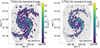 |
Fig. 1. Integrated intensity (moment-0) maps of the 13CO(1−0) (left) and C18O(1−0) (right) emission lines. Grey points denote non-detections, i.e. sightlines with S/N ≤ 3, while coloured points indicate detections with S/N > 3. Overlaid contours correspond to the 12CO(1−0) emission (Pety et al. 2013) at the 30 K km s−1 level, shown for reference. |
2. Data
The SWAN survey, an IRAM large program (LP003; PIs: F. Bigiel, E. Schinnerer), used the NOrthern Extended Millimetre Array (NOEMA) and the IRAM 30-meter telescope to map 3−4 mm emission lines in M51 at a spatial resolution of 3″ (≈125 pc) over the central 5 × 7 kpc2. For a more detailed description of the observations and data reduction, see Appendix A in Stuber et al. (2023, 2025). Additional data include Spitzer 24 μm maps from Dumas et al. (2011) and the Hα maps from Kessler et al. (2020), combined using Eq. (6) from Leroy et al. (2013) to create a ΣSFR map (see middle panel in Fig. 2), as well as the 12CO(1−0) map from the PdBI Arcsecond Whirlpool Survey (PAWS; Schinnerer et al. 2013). For our environmental analysis we used a simplified version of the PAWS environmental mask (Colombo et al. 2014b) based on the underlying stellar potential. We did not account for dynamically distinct sub-regions within the spiral arms or interarm regions; instead, we considered only the following broader environments (see right panel in Fig. 2): the nuclear bar, the molecular ring, the northern arm, the southern arm, and the interarm. For ease of comparison to lower-resolution works, we also grouped these environments into two more general categories of the centre (defined as R < 1.3 kpc, containing the nuclear bar and molecular ring) and the disc (1.3 kpc < R < 5 kpc, containing both spiral arms and the interarm region). Using the PyStructure code (Neumann et al. 2023a), the datasets were convolved to the same spatial resolution of 3.05″ and spectral resolution of 10 km s−1 for CO and its isotopologues before a half-beam-sized sampling was applied. Moment maps were created by integrating voxels where 12CO or HCN was detected, with the detected region defined using a 3D mask with thresholds of S/N > 4 expanded to S/N > 2. Since the influence of the AGN on the CO isotopologues is not yet well understood, we masked the central region to avoid introducing potential biases into our analysis. A more detailed discussion of this decision is provided in Sect. 4.2. Specifically, we excluded the inner 500 pc, which encompasses the AGN radio jets (Querejeta et al. 2016b). Although checks based on the ionization state of the gas – following the methodology of D’Agostino et al. (2019) – suggest that masking the inner 300 pc would suffice, we adopted a more conservative approach by extending the exclusion to 500 pc to ensure minimal contamination from possible AGN-related effects.
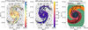 |
Fig. 2. Complete dataset; the version masked for AGN activity and used in the analysis is provided in Appendix C. The left panel shows the |

3. Results
3.1. Ratio of medians
In this paper, we focus on  as a way to trace variations in the isotopic abundance and opacity in molecular clouds, particularly in relation to star formation (SF) activity and galactic structure. Figure 2 (left) displays a map of
  across M51. For sightlines where both lines have S/N > 3, the 16th and 84th percentiles extend from 3.4 and 5.2, respectively. To understand how
  varies between environments and how this local behaviour compares to the galaxy-averaged behaviour, we calculated the ratio of medians both for the entire field of view (FoV) and for each specific environment using the following equation:
 (1)
(1)
where  and
and  represent the median integrated intensities of 13CO and C18O lines, respectively. We chose to use the ratio of median integrated intensities rather than the median of individual integrated intensity ratios, as this approach is less sensitive to C18O detectability. When C18O is faint or undetected, pixel-wise ratios can become artificially large, skewing the median of ratios. While applying a signal-to-noise cut could mitigate this, it would bias the analysis towards bright regions and misrepresent the full FoV. By using the ratio of medians without S/N cuts, we retained information from low-S/N sightlines while minimizing the impact of outliers. Specifically for the SWAN data, the relative difference1 between the median of ratios and ratio of medians across the entire FoV is approximately 11% of the ratio of medians value. When broken down by environment, the difference decreases to just 1−3%, except in the southern spiral arm, where it increases to 21%. For more information on the median of ratios and its uncertainties, see Appendix D.
We applied Eq. (1) to the data, with the propagated statistical uncertainty calculated by combining  and
and  uncertainties using standard error propagation. The results are summarized in Table 1. We now compare our results to values reported in the literature, noting that some of the referenced studies use different methodologies (e.g. the median of ratios rather than the ratio of medians). In such cases, the uncertainties provided in Table 1 should be taken into account when assessing the level of agreement. The resulting
  across the FoV is 4.33 ± 0.05, which aligns well with the results of den Brok et al. (2022), who used the IRAM 30 m telescope to map ≈15 × 15 kpc2 of M51 at a kiloparsec-scale resolution, reporting an average ratio of
  . For the centre, we find a
  of 3.98 ± 0.02, while for the disc, it is 4.8 ± 0.1, resulting in a relative difference of 20% of the central value. The central value is close to the 3.6 ± 0.3 reported by Vila-Vilaró (2008), who found the ratio based on single-point observation of the inner 950 pc using the ARO Kitt Peak 12 m telescope. Similarly, Tan et al. (2011), who mapped M51’s major axis with 13 pointings using the PMO 14 m telescope, found a ratio of 3.7 for the nucleus. However, their reported ratio of 2.6 for the disc differs from our findings. Jiménez-Donaire et al. (2017) observed the ratio ranging from 7 to 10 in the discs of nine nearby normal star-forming galaxies, which are significantly higher than our disc ratio. For galactic centres, they report ratios between 3.8 and 8.7, which are more consistent with our central value. In the Milky Way, ratios reported by Langer & Penzias (1990) and Wouterloot et al. (2008) span from 5 to 10, also exceeding the values we find for M51 in both the disc and the centre. When examining individual environments, the southern spiral arm exhibits a notably higher
  , approximately 24% above the FoV value, while the other environments show an average deviation of only 9%. This deviation in the southern arm does not appear to be purely statistical, given its similar number of data points and scatter level compared to the northern arm, which does not exhibit a similar trend. Additionally,
  is not the only line ratio exhibiting such behaviour; Stuber et al. (2023) report an elevated N2H+(1−0)/HCN(1−0) ratio in the same area of the southern arm. This suggests that the variation may have a physical origin.
 and median ΣSFR by region.
A potential explanation for these elevated line ratios could involve the difference in ΣSFR between the arms, with the northern arm having a 25% larger ΣSFR than the southern one. Meidt et al. (2013) and Querejeta et al. (2016b) have shown that the southern arm has a reduced star formation efficiency (SFE) due to strong streaming motions stabilizing the gas. The  in the nuclear bar and the molecular ring, on the other hand, fall within the ranges typically observed for starbursts (3 to 6; Sage et al. 1991; Aalto et al. 1995) and on the higher end for ULIRGs (0.2 to 4; Sliwa et al. 2017; Brown & Wilson 2019).
3.2. R in different environments
To investigate how  varies with local environmental conditions, we compared the ratio with the galactocentric radius and ΣSFR. These parameters were selected because they effectively capture potential gradients in physical and chemical conditions. Specifically, SF can influence the chemical enrichment and excitation conditions of the gas, while factors such as gas-phase metallicity are known to vary with radius. To quantify the correlation between
  and either galactocentric radius or ΣSFR, we used Kendall’s τ. This non-parametric method is well suited for our data as it minimizes bias from outliers and accommodates the non-normal distribution of ratio values. We computed Kendall’s tau for both the entire FoV and each environment. We present two methods of doing this – one uses only points with a S/N > 3 (shown as coloured points in Figs. 3 and 4) and the other uses spectrally stacked (see Appendix A for details) points with S/N > 3 (shown as hexagonal points in Figs. 3 and 4). The resulting correlation coefficients (τ) are presented in Table 2. For the stacking analysis, we tested using 6, 8, 10, and 12 bins to evaluate the stability of the correlation coefficients. We found that the choice of bin number had no significant effect on the overall trends. Specifically, using 10 bins resulted in relative differences of 11%, 10%, and 0.04% compared to results obtained with 12, 8, and 6 bins, respectively. Based on this, we adopted 10 bins as a representative and stable choice. For reference, we categorize correlation coefficients as follows: values between 0.1 and 0.4 are considered low, 0.4 to 0.7 as moderate, and values above 0.7 as high.
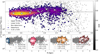 |
Fig. 3.
|


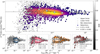 |
Fig. 4.
|

Correlation coefficients between  and environment.
Galactocentric radius. The top panel in Fig. 3 illustrates how  varies with distance from the galactic centre. Sightlines where both 13CO(1−0) and C18O(1−0) have S/N > 3 are shown as coloured points, while the grey points seen in the background of the panel have one or both lines with S/N ≤ 3. If 13CO(1−0) is not detected, it indicates an upper limit, whereas if C18O(1−0) is not detected, it indicates a lower limit. The scatter of all points is ≈0.4 dex. With τ = 0.22 (p value ≪ 0.05), the FoV shows a low correlation between the ratio and radius. When calculated from the stacked points, the correlation coefficient increases to τ = 0.71 (p value = 0.06), suggesting a high correlation.
SFR surface density. We additionally investigated  as a function of ΣSFR in Fig. 4 and found a negative trend. However, the scatter at low ΣSFR also increases as we approach the detection limits of the CO isotopologues and SFR. We observe a low negative correlation across the FoV with τ = −0.18 (p value ≪ 0.05) and a stronger negative trend of τ = −0.86 (p value ≪ 0.05) when using the stacked points. Examining individual environments, the point-based method yields low correlations with statistically significant p values, expect for the nuclear bar and northern arm, which show no correlation. These correlations are negative in all regions except for the southern spiral arm. In contrast, the stacked method indicates high correlation coefficients with significant p values for the molecular ring and northern spiral arm, while the nuclear bar and southern spiral arm exhibit low to moderate correlation coefficients with high p values.
While there is significant scatter and the actual median ratio varies roughly by 68% with radius in the inner 3.2 kpc and by 30% with ΣSFR for ΣSFR > 0.02, formally we find a correlation between the ratio and galactocentric radius, as well as an anti-correlation with ΣSFR. We calculated these variations by determining the median ratio within each bin shown in Figs. 3 and 4, then dividing the difference between the maximum and minimum bin median ratios by the median ratio of the entire dataset. The observed trends are consistent with findings from Jiménez-Donaire et al. (2017) and den Brok et al. (2022) at kiloparsec resolution. While we cannot precisely determine the strength of these correlations, we can establish some constraints on their values. The correlation coefficients from the stacked spectra are higher than those from the pixel-by-pixel analysis, primarily because stacking averages out noise and astrophysical scatter. The pixel-by-pixel method retains more local variability, leading to greater scatter in the correlations. Comparing our correlation coefficients from stacked points to those of den Brok et al. (2022), we find that they report a slightly higher correlation coefficient of 0.8 (p = 0.083) for galactocentric radius, likely due to their extended detection range up to 5 kpc capturing higher ratio values. In the case of ΣSFR, they find a correlation of −0.67 (p = 0.33), which is lower than our value but has a higher p value. While differences likely arise due to mismatched spatial scales, the trends alignqualitatively.
4. Discussion
The observed trends with  may be explained by abundance-driven variations resulting from processes such as selective nucleosynthesis, chemical fractionation, and selective photodissociation. Alternatively, changes in the opacities of both species with their abundances fixed or variations in line excitation could also account for these observed patterns. In this section we explore the likelihood of those explanations for our observed trends.
4.1. Variations in line excitation
Previous studies conducted at kiloparsec scales (den Brok et al. 2022), along with more recent investigations (den Brok et al. 2025) utilizing CO multi-line datasets from SMA, SWAN, and PAWS data at a spatial resolution of 4″ (≈170 pc), both conclude that, on global scales, variations in line excitation do not significantly affect the line ratios.
4.2. Variations in molecular abundances
Chemical fractionation. In cold regions, the abundances of 13CO and C18O molecules can be affected by chemical fractionation (Watson et al. 1976; Smith & Adams 1980; Keene et al. 1998; Romano et al. 2017), which enhances the production of 13CO at the expense of 12CO via the exothermic reaction

where ΔE represents the energy change associated with the reaction. Langer et al. (1984) note that the fractionation reaction for C18O,

is unlikely to occur since it has a small rate coefficient at 300 K and a substantial activation energy barrier. This makes the reaction inefficient at the low temperatures where 13CO fractionation is observed. Therefore, in a simple scenario where ΣSFR traces temperature, we would expect a high  in cold regions with low ΣSFR, as is shown in Fig. 3. Szűcs et al. (2014) have performed hydrodynamical simulations of molecular clouds and found that chemical fractionation can decrease 12CO(1−0)/13CO(1−0) (
 ) by a factor of 2−3 at low temperatures and optical depths. We would then expect
  to increase with ΣSFR, but upon examining Fig. B.2 we find that this is not the case on a galaxy-wide scale. Therefore, we conclude that this chemical reaction is unlikely to be the driver of the observed trends for
  . These results are consistent with those of Cormier et al. (2018), who found a mild anti-correlation between
  and both dust temperature and ΣSFR in M51.
Selective photodissociation. The UV radiation from O and B stars, traced by regions of high SFR surface density, preferentially photodissociates 13CO and C18O compared to 12CO molecules due to their poorer self-shielding capabilities resulting from lower abundances (van Dishoeck & Black 1988; Lyons & Young 2005). Since 13CO is slightly more abundant than C18O, it is less susceptible to photodissociation, leading to a higher  ratio as ΣSFR increases. This process should also cause
  to increase with ΣSFR. However, Fig. B.2 reveals that
  decreases with ΣSFR in M51, suggesting that selective photodissociation is also an unlikely contributor to the observed trends.
Selective nucleosynthesis. Stars of varying masses and ages enrich the ISM with different CO isotopologues (Henkel & Mauersberger 1993; Casoli et al. 1992), making these molecules valuable indicators of a galaxy’s evolutionary stage. Specifically, 13C is synthesized during the helium-burning phase of intermediate-mass stars, while 18O and 12C are produced in supernova explosions of high-mass stars. If selective nucleosynthesis were driving the observed trends, we would expect increased C18O production in regions of high ΣSFR, thereby lowering  . Furthermore, by observing nine interstellar clouds in the Galaxy, Langer & Penzias (1990) and Milam et al. (2005) found that 12C/13C and 16O/18O ratios increase from the galactic centre, which is attributed to the inside-out formation of galaxies. This is consistent with the trends we observe for the plots in Appendices A and B and Fig. 4.
4.3. Variations in opacity
Another potential explanation for the observed trends is opacity variations of the lines across the FoV. This was investigated in den Brok et al. (2025), where the optical depth of 13CO(1−0) is derived under both LTE and non-LTE conditions. The 13CO optical depth map presented in the study shows an increase in opacity towards the galaxy’s centre (≈0.1−0.6), leading to a lower emissivity of 13CO gas in the central region. This reduction in 13CO emission decreases  , potentially explaining the radial trend we observe. To quantify this effect, we used the solution to the radiative transfer equation. Assuming no background intensity, similar excitation conditions and similar beam filling factors between the two molecular lines, we arrived at the following expression: I1/I2 = (1 − e−τ1)/(1 − e−τ2), where τi represents the optical depth and Ii the integrated intensity of each line. To quantify the impact of optical depth, we assumed a fixed [13CO]/[C18O] abundance ratio across the FoV. In the disc, 13CO is optically thin according to den Brok et al. (2025), who report
  . Under these assumptions, the above equation simplifies to I1/I2 ≈ τ1/τ2, and since τ1/τ2 = X1/X2 we obtain X13/X18 ≈ 4.8 ± 0.1. In the centre, 13CO becomes partially optically thick, with an average
  . Using
  , we obtain
  . Substituting these optical depths back into the above equation yields I13/I18 ≈ 3.8387 ± 0.0002 for the centre, which is slightly lower than the 3.98 ± 0.02 from observations. This suggests that changes in optical depth could contribute to the observed
  trends. We extended this analysis to the 12CO/13CO ratio, assuming 12CO to be optically thick across the entire FoV. For the disc, we calculated that
  , while for the centre we got
  . From observations, we found that I12/I13 = 10.89 ± 0.07 for the disc and I12/I13 = 6.96 ± 0.02 for the centre. The calculated disc value aligns well with the observed ratio, supporting the assumption of optically thin 13CO and thick 12CO in this region. However, the observed central ratio significantly exceeds the predicted value, suggesting the influence of additional processes driving the ratio higher in the central region. Paglione et al. (2001) demonstrated that a higher velocity dispersion, elevated gas kinetic temperature, or lower gas column density can reduce the optical depth of 12CO, thereby enhancing its intensity. Teng et al. (2024) similarly find that dynamical effects can lower the 12CO optical depth. Physical processes such as turbulence or the presence of bars in galaxy centres can drive these conditions, potentially leading to an increase in
  (Paglione et al. 2004; Israel 2009a,b; Cormier et al. 2018).
4.4. Outliers from average trends
To evaluate deviations from the average trends, we calculated the offset of statistically significant sightlines from both the FoV-wide ratio of medians as well as from the stacked values (grey hexagons in Figs. 3 and 4), which represent an unbiased average of the ratio as a function of galactocentric radius and ΣSFR. We refer to these offsets from average values as ΔR. For a sightline, i, the ΔR from the FoV-wide ratio of medians was determined as
 (2)
(2)
where  is the ratio of sightline i and
  is the FoV-wide ratio of medians. The variation in the ratio for sightline j relative to the spectrally stacked value in the corresponding ΣSFR bin was calculated as
 (3)
(3)
where  is the ratio for sightline j and
  is the spectrally stacked ratio of all sightlines in the ΣSFR bin which contains sightline j. The scatter around this trend is considerable, with a typical deviation of ≈1 and a maximum deviation of ≈4.5, indicating that some sightlines reach up to twice the average ratio. The spatial distribution of these ‘outliers’ is shown in Fig. 5: the left panel shows deviations from the FoV-wide ratio of medians, while the right panel shows deviations from the ΣSFR stacked value in a corresponding bin. These maps clearly highlight regions with elevated or suppressed ratios across the FoV. The high Δ values in the northern arm align with regions of high ΣSFR, suggesting a link to star formation activity, while a notable depletion is visible in the southern arm. As was already seen in the ratio map in Fig. 5, the north-west side of the molecular ring shows a noticeably different characteristic ratio compared to the southeast side. This asymmetry remains evident even after controlling for ΣSFR, indicating that this feature cannot be explained by star formation alone. Instead, it likely arises from other physical processes such as gas outflows or dynamical disturbances.
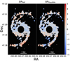 |
Fig. 5. Deviations of significant (S/N > 3) points from the average trends. The left panel illustrates the deviation of significant data points from the ratio of medians for the entire FoV, while the right panels show how these significant points deviate from the stacked average within the corresponding ΣSFR bin for the full FoV. |
We conclude that abundance variations from selective nucleosynthesis and/or changes in the opacity of the gas are the most likely drivers of the observed trends with radius and ΣSFR. While our study benefits from a high spatial resolution and from multiple lines compared to earlier work, our limited spatial coverage imposes a restriction. Expanding our observations to encompass larger radii and lower SFR regions could better constrain the strength of the correlations we find. Additionally, our current approach to calculating ΣSFR relies on a combination of 24 μm and Hα emission, which, as is reported by Calzetti et al. (2024), can vary depending on the mean age of the stellar populations contributing to dust heating.
5. Summary
We present 13CO(1−0) and C18O(1−0) observations of the inner 5 × 7 kpc2 of M51 from the SWAN survey. We analysed the ratio of these lines against both the galactocentric radius and the SFR surface density across the SWAN FoV, as well as within distinct environments encompassed by the FoV.
Our key findings are as follows:
-
The ratio of medians for the FoV is
 .
. -
The ratio shows a low positive correlation with galactocentric radius.
-
The ratio shows a low negative correlation with ΣSFR, particularly within the molecular ring and northern spiral arm.
-
There is a notable difference in behaviour between the northern and southern spiral arms, as was expected from previous studies of the spiral structure in M51.
-
The ratio trends are most likely driven by a combination of selective nucleosynthesis and optical depth effects.
M51 provides valuable insights into the factors influencing CO isotopologues within a grand design spiral galaxy. It is evident that SF and environment play a role in this. Extension of such multi-line, high-resolution mapping of other galaxies could potentially reveal additional environmental dependencies across a wider range of SFR and radius values.
Calculated as  , where xref denotes the corresponding ratio of medians.
Acknowledgments
This work was carried out as part of the PHANGS collaboration. This work is based on data obtained by PIs E. Schinnerer and F. Bigiel with the IRAM-30 m telescope and NOEMA observatory under project ID M19AA. This research was conducted with the support of the International Max Planck Research School (IMPRS) for Astronomy and Astrophysics at the universities of Bonn and Cologne. JEMD acknowledges support from project UNAM DGAPA-PAPIIT IG 101025, Mexico. ES acknowledges funding from the European Research Council (ERC) under the European Union’s Horizon 2020 research and innovation programme (grant agreement No. 694343). SKS acknowledges financial support from the German Research Foundation (DFG) via Sino-German research grant SCHI 536/11-1. JPe acknowledges support by the French Agence Nationale de la Recherche through the DAOISM grant ANR-21-CE31-0010 and by the Programme National “Physique et Chimie du Milieu Interstellaire” (PCMI) of CNRS/INSU with INC/INP, co-funded by CEA and CNES. MJJD, AU and MQ acknowledge support from the Spanish grant PID2022-138560NB-I00, funded by MCIN/AEI/10.13039/501100011033/FEDER, EU. JdB acknowledges support from the Smithsonian Institution as a Submillimeter Array (SMA) Fellow. JEMD gratefully acknowledges funding from the Deutsche Forschungsgemeinschaft (DFG, German Research Foundation) in the form of an Emmy Noether Research Group (grant number KR4598/2-1, PI Kreckel) and the European Research Council’s starting grant ERC StG-101077573 (“ISM-METALS”). HAP acknowledges support from the National Science and Technology Council of Taiwan under grants 110-2112-M-032-020-MY3 and 113-2112-M-032-014-MY3. TAD acknowledges support from the UK Science and Technology Facilities Council through grant ST/W000830/1.
References
- Aalto, S., Booth, R. S., Black, J. H., & Johansson, L. E. B. 1995, A&A, 300, 369 [NASA ADS] [Google Scholar]
- Aladro, R., Viti, S., Bayet, E., et al. 2013, A&A, 549, A39 [NASA ADS] [CrossRef] [EDP Sciences] [Google Scholar]
- Brown, T., & Wilson, C. D. 2019, ApJ, 879, 17 [NASA ADS] [CrossRef] [Google Scholar]
- Calzetti, D., Adamo, A., Linden, S. T., et al. 2024, ApJ, 971, 118 [Google Scholar]
- Casoli, F., Dupraz, C., & Combes, F. 1992, A&A, 264, 55 [NASA ADS] [Google Scholar]
- Colombo, D., Meidt, S. E., Schinnerer, E., et al. 2014a, ApJ, 784, 4 [Google Scholar]
- Colombo, D., Hughes, A., Schinnerer, E., et al. 2014b, ApJ, 784, 3 [NASA ADS] [CrossRef] [Google Scholar]
- Cormier, D., Bigiel, F., Jiménez-Donaire, M. J., et al. 2018, MNRAS, 475, 3909 [NASA ADS] [CrossRef] [Google Scholar]
- Costagliola, F., Aalto, S., Rodriguez, M. I., et al. 2011, A&A, 528, A30 [NASA ADS] [CrossRef] [EDP Sciences] [Google Scholar]
- Crocker, A., Krips, M., Bureau, M., et al. 2012, MNRAS, 421, 1298 [NASA ADS] [CrossRef] [Google Scholar]
- D’Agostino, J. J., Kewley, L. J., Groves, B. A., et al. 2019, MNRAS, 485, L38 [CrossRef] [Google Scholar]
- Davis, T. A. 2014, MNRAS, 445, 2378 [NASA ADS] [CrossRef] [Google Scholar]
- Davis, T. A., Bayet, E., Crocker, A., Topal, S., & Bureau, M. 2013, MNRAS, 433, 1659 [Google Scholar]
- Davis, T. A., Gensior, J., Bureau, M., et al. 2022, MNRAS, 512, 1522 [CrossRef] [Google Scholar]
- den Brok, J. S., Bigiel, F., Sliwa, K., et al. 2022, A&A, 662, A89 [CrossRef] [EDP Sciences] [Google Scholar]
- den Brok, J. S., Leroy, A. K., Usero, A., et al. 2023, MNRAS, 526, 6347 [Google Scholar]
- den Brok, J., Jiménez-Donaire, M. J., Leroy, A., et al. 2025, AJ, 169, 18 [Google Scholar]
- Donovan Meyer, J., Koda, J., Momose, R., et al. 2013, ApJ, 772, 107 [NASA ADS] [CrossRef] [Google Scholar]
- Dumas, G., Schinnerer, E., Tabatabaei, F. S., et al. 2011, AJ, 141, 41 [NASA ADS] [CrossRef] [Google Scholar]
- Egusa, F., Gao, Y., Morokuma-Matsui, K., Liu, G., & Maeda, F. 2022, ApJ, 935, 64 [NASA ADS] [CrossRef] [Google Scholar]
- He, H., Wilson, C. D., Sun, J., et al. 2024, ArXiv e-prints [arXiv:2401.16476] [Google Scholar]
- Henkel, C., & Mauersberger, R. 1993, A&A, 274, 730 [NASA ADS] [Google Scholar]
- Ho, L. C., Filippenko, A. V., & Sargent, W. L. W. 1997, ApJS, 112, 315 [NASA ADS] [CrossRef] [Google Scholar]
- Israel, F. P. 2009a, A&A, 493, 525 [NASA ADS] [CrossRef] [EDP Sciences] [Google Scholar]
- Israel, F. P. 2009b, A&A, 506, 689 [NASA ADS] [CrossRef] [EDP Sciences] [Google Scholar]
- Jiménez-Donaire, M. J., Cormier, D., Bigiel, F., et al. 2017, ApJ, 836, L29 [Google Scholar]
- Keene, J., Schilke, P., Kooi, J., et al. 1998, ApJ, 494, L107 [NASA ADS] [CrossRef] [Google Scholar]
- Kennicutt, R. C., & Evans, N. J. 2012, ARA&A, 50, 531 [NASA ADS] [CrossRef] [Google Scholar]
- Kessler, S., Leroy, A., Querejeta, M., et al. 2020, ApJ, 892, 23 [NASA ADS] [CrossRef] [Google Scholar]
- Koda, J., Hirota, A., Egusa, F., et al. 2023, ApJ, 949, 108 [NASA ADS] [CrossRef] [Google Scholar]
- Krips, M., Crocker, A. F., Bureau, M., Combes, F., & Young, L. M. 2010, MNRAS, 407, 2261 [Google Scholar]
- Langer, W. D., & Penzias, A. A. 1990, ApJ, 357, 477 [Google Scholar]
- Langer, W. D., Graedel, T. E., Frerking, M. A., & Armentrout, P. B. 1984, ApJ, 277, 581 [Google Scholar]
- Leroy, A. K., Walter, F., Sandstrom, K., et al. 2013, AJ, 146, 19 [Google Scholar]
- Lyons, J. R., & Young, E. D. 2005, Nature, 435, 317 [Google Scholar]
- McQuinn, K. B. W., Skillman, E. D., Dolphin, A. E., Berg, D., & Kennicutt, R. 2016, ArXiv e-prints [arXiv:1610.03857] [Google Scholar]
- Meidt, S. E., Schinnerer, E., García-Burillo, S., et al. 2013, ApJ, 779, 45 [NASA ADS] [CrossRef] [Google Scholar]
- Meier, D. S., & Turner, J. L. 2004, AJ, 127, 2069 [CrossRef] [Google Scholar]
- Milam, S. N., Savage, C., Brewster, M. A., Ziurys, L. M., & Wyckoff, S. 2005, ApJ, 634, 1126 [Google Scholar]
- Neumann, L., Gallagher, M. J., Bigiel, F., et al. 2023a, MNRAS, 521, 3348 [NASA ADS] [CrossRef] [Google Scholar]
- Neumann, L., den Brok, J. S., Bigiel, F., et al. 2023b, A&A, 675, A104 [NASA ADS] [CrossRef] [EDP Sciences] [Google Scholar]
- Paglione, T. A. D., Wall, W. F., Young, J. S., et al. 2001, ApJS, 135, 183 [NASA ADS] [CrossRef] [Google Scholar]
- Paglione, T. A. D., Yam, O., Tosaki, T., & Jackson, J. M. 2004, ApJ, 611, 835 [NASA ADS] [CrossRef] [Google Scholar]
- Peñaloza, C. H., Clark, P. C., Glover, S. C. O., Shetty, R., & Klessen, R. S. 2017, MNRAS, 465, 2277 [CrossRef] [Google Scholar]
- Pereira-Santaella, M., Colina, L., García-Burillo, S., et al. 2021, A&A, 651, A42 [NASA ADS] [CrossRef] [EDP Sciences] [Google Scholar]
- Pety, J., Schinnerer, E., Leroy, A. K., et al. 2013, ApJ, 779, 43 [NASA ADS] [CrossRef] [Google Scholar]
- Querejeta, M., Meidt, S. E., Schinnerer, E., et al. 2016a, A&A, 588, A33 [NASA ADS] [CrossRef] [EDP Sciences] [Google Scholar]
- Querejeta, M., Schinnerer, E., García-Burillo, S., et al. 2016b, A&A, 593, A118 [NASA ADS] [CrossRef] [EDP Sciences] [Google Scholar]
- Romano, D., Matteucci, F., Zhang, Z. Y., Papadopoulos, P. P., & Ivison, R. J. 2017, MNRAS, 470, 401 [NASA ADS] [CrossRef] [Google Scholar]
- Sage, L. J., Mauersberger, R., & Henkel, C. 1991, A&A, 249, 31 [NASA ADS] [Google Scholar]
- Sanders, D. B., Scoville, N. Z., & Solomon, P. M. 1985, ApJ, 289, 373 [NASA ADS] [CrossRef] [Google Scholar]
- Sawada, T., Hasegawa, T., Handa, T., et al. 2001, ApJS, 136, 189 [NASA ADS] [CrossRef] [Google Scholar]
- Schinnerer, E., Meidt, S. E., Pety, J., et al. 2013, ApJ, 779, 42 [Google Scholar]
- Shirley, Y. L. 2015, PASP, 127, 299 [Google Scholar]
- Sliwa, K., Wilson, C. D., Aalto, S., & Privon, G. C. 2017, ApJ, 840, L11 [Google Scholar]
- Smith, D., & Adams, N. G. 1980, ApJ, 242, 424 [Google Scholar]
- Stuber, S. K., Pety, J., Schinnerer, E., et al. 2023, A&A, 680, L20 [NASA ADS] [CrossRef] [EDP Sciences] [Google Scholar]
- Stuber, S. K., Pety, J., Usero, A., et al. 2025, A&A, 696, A182 [NASA ADS] [CrossRef] [EDP Sciences] [Google Scholar]
- Szűcs, L., Glover, S. C. O., & Klessen, R. S. 2014, MNRAS, 445, 4055 [CrossRef] [Google Scholar]
- Tan, Q.-H., Gao, Y., Zhang, Z.-Y., & Xia, X.-Y. 2011, RAA, 11, 787 [Google Scholar]
- Tang, X. D., Henkel, C., Menten, K. M., et al. 2017, A&A, 598, A30 [NASA ADS] [CrossRef] [EDP Sciences] [Google Scholar]
- Teng, Y.-H., Sandstrom, K. M., Sun, J., et al. 2023, ApJ, 950, 119 [NASA ADS] [CrossRef] [Google Scholar]
- Teng, Y.-H., Chiang, I.-D., Sandstrom, K. M., et al. 2024, ApJ, 961, 42 [NASA ADS] [CrossRef] [Google Scholar]
- Topal, S., Bureau, M., Davis, T. A., et al. 2016, MNRAS, 463, 4121 [Google Scholar]
- van Dishoeck, E. F., & Black, J. H. 1988, ApJ, 334, 771 [Google Scholar]
- Vila-Vilaró, B. 2008, PASJ, 60, 1231 [Google Scholar]
- Watson, W. D., Anicich, V. G., & Huntress, W. T. 1976, ApJ, 205, L165 [NASA ADS] [CrossRef] [Google Scholar]
- Wilson, T. L., & Rood, R. 1994, ARA&A, 32, 191 [Google Scholar]
- Wilson, C. D., Walker, C. E., & Thornley, M. D. 1997, ApJ, 483, 210 [CrossRef] [Google Scholar]
- Wouterloot, J. G. A., Henkel, C., Brand, J., & Davis, G. R. 2008, A&A, 487, 237 [NASA ADS] [CrossRef] [EDP Sciences] [Google Scholar]
- Yoda, T., Handa, T., Kohno, K., et al. 2010, PASJ, 62, 1277 [NASA ADS] [Google Scholar]
Appendix A: Spectral stacking
Spectral stacking is a method used to improve the signal-to-noise ratio of faint emission lines, such as C18O(1-0) in our case, by aligning and averaging spectra from different regions. To achieve this, we used the PyStacker code (Neumann et al. 2023b) on the dataset. The code bins the spectra based on a specific quantity, such as galactocentric radius or SFR surface density, and then averages them to improve the overall S/N. A critical step in this process is aligning the spectra to ensure there is no velocity offset between them. This is achieved by shifting each spectrum to a common velocity frame, typically defined by a high-S/N reference line like 12CO(1−0) or HI 21 cm. In our case, the 12CO(1−0) line was used as a prior to define the velocity field for the stacking. This velocity alignment ensures that the emission lines from different regions of the galaxy are centred at 0 km/s. Once aligned, the spectra are averaged by summing the shifted spectra and dividing by the number of spectra in the bin. In Figs. 3-4, the stacked points were created by dividing the stacked 13CO(1-0) stacks by the C18O(1-0) ones. If both stacked lines had an S/N > 3, the point was considered a detection and marked as a hexagonal point on the plot. If the ratio error (computed by propagating the statistical uncertainty of each line) was lower than or equal to 3 and the line in the denominator (C18O) had S/N ≤ 3, the point was marked with a upward triangle and indicated a lower limit. If the line in the numerator (13CO) had S/N ≤ 3, it was marked with a downward triangle and indicated an upper limit. Lines where both the ratio error and individual S/N were lower than or equal to 3 were considered non-detections and marked with diamond points. In our correlation coefficient calculations using Kendall’s tau, non-detected and limit stacked points were excluded. These steps help ensure that the stacked spectra accurately represent the underlying emission, while excluding unreliable data points.
Appendix B: Alternative line ratios and their implications
Analogous to our analysis of the 13CO(1-0) to C18O(1-0) ratio, we also examine the 12CO(1-0) to 13CO(1-0) and 12CO(1-0) to C18O(1-0) ratios. Among these, the 12CO/13CO ratio offers the most extensive coverage of the galaxy, as both 12CO(1-0) and 13CO(1-0) are detected with high significance. The ratios of medians for these alternative line ratios are summarized in Table B.1. Across the entire FoV, 12CO(1-0) is typically ≈ 9 times brighter than 13CO(1-0) and ≈ 40 times brighter than C18O(1-0). Consistent with the behaviour of the 13CO/C18O ratio, the ratio of medians in the central region is lower than in the disc, with a relative difference of 56% for 12CO/13CO and 88% for 12CO/C18O. Additionally, variations between spiral arms are also evident for these ratios: the northern arm exhibits a 16% lower ratio of medians for 12CO/13CO and a 28% lower value for 12CO/C18O compared to the southern arm. We applied the same methods described in Sect. 3.2 to calculate Kendall’s τ correlation coefficients between the ratios and both galactocentric radius and ΣSFR. For the radius relations, we observe moderate positive correlations when using the pixel-by-pixel method and a strong positive correlation when using the stacked method. For the pixel-by-pixel analysis across the entire FoV and each environment, we observe a low anti-correlation between both ratios and ΣSFR. When using stacked data, 12CO/13CO ratio shows a low anti-correlation, while the 12CO/C18O ratio exhibits a moderate anti-correlation for the FoV, but the p values for these coefficients are much higher than the 0.05 threshold. When looking at individual environments, we find that the nuclear bar remains uncorrelated while the molecular ring has a high anti-correlation both for the main and the alternative ratios. Interestingly, the southern spiral arm shows a strong anti-correlation with ΣSFR for these ratios, in contrast to the 13CO/C18O ratio, where no such correlation is found.
Ratio of medians for 12CO(1-0)/13CO(1-0) and 12CO(1-0)/C18O(1-0) by region.
Kendall’s rank correlation coefficient between 12CO(1-0)/13CO(1-0) ratio and ΣSFR.
Kendall’s rank correlation coefficient between 12CO(1-0)/C18O(1-0) ratio and ΣSFR.
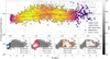 |
Fig. B.1. 12CO(1-0) to 13CO(1-0) line ratio plotted against the galactocentric radius. The description is analogous to that in Fig.3. |
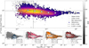 |
Fig. B.2. 12CO(1-0) to 13CO(1-0) line ratio plotted against the SFR surface density. The description is analogous to that in Fig.4. |
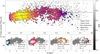 |
Fig. B.3. 12CO(1-0) to C18O(1-0) line ratio plotted against the galactocentric radius. The description is analogous to that in Fig.3. |
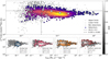 |
Fig. B.4. 12CO(1-0) to C18O(1-0) line ratio plotted against the ΣSFR. The description is analogous to that of Fig.4. |
Appendix C: Assessing AGN influence on R
Enhanced UV radiation and cosmic ray fluxes from the AGN may alter the local chemistry, potentially affecting the isotopologue ratios. While 13CO is more abundant and capable of self-shielding, C18O is more easily photodissociated, which could lead to a slight increase in the 13CO/C18O ratio. However, the elevated temperatures in the AGN vicinity likely suppress chemical fractionation processes, which are more efficient in cold gas. Additionally, AGN-driven changes in ion-formation pathways could influence molecular abundances, though the detailed chemistry under such extreme conditions remains uncertain. A more detailed investigation of AGN effects on the SWAN line ratios will be presented in upcoming studies by Usero et al. (in prep.) and Thorp et al. (in prep.).
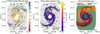 |
Fig. C.1. Description is analogous to Fig.2. The white regions in the centre of the galaxy are the regions masked for the AGN activity. |
Appendix D: Alternative ratio averaging methods and their uncertainties
Comparison of ratio of medians and median of ratios per environment.
In Sect. 3.1 we explained our preference for using the ratio of medians over the median of ratios, primarily due to the impact of C18O detectability. The median of ratios method assigns equal weight to each individual ratio which allows low-quality data, specifically pixels with faint C18O emission, to disproportionately influence the final result. Nevertheless, for completeness and ease of comparison to other works, we also present the results using the median of ratios method in this section. The median of ratios is computed by first calculating the ratio on a pixel-by-pixel basis, after which the final value is taken as the median of all valid individualratios:
 (D.1)
(D.1)
where x and y are integrated intensities of the two tracers (e.g. 13CO and C18O). Since we do not censor our data, the propagated uncertainty of the median of ratios exhibits unrealistically high values. To address this, we introduce two alternative methods for estimating the characteristic variation of median of ratios. The first indicator is the median absolute deviation (MAD) of the distribution of pixel-wise ratio uncertainties. For each pixel, the uncertainty in the ratio, MRi, is calculated using standard error propagation on the individual uncertainties σxi and σyi of xi and yi, respectively:
 (D.2)
(D.2)
The resulting MADs are listed in the third column of Table D.1, alongside the corresponding medians of ratios for each region. The second indicator is obtained through bootstrapping; we generate subsamples of the ratio dataset, allowing repetitions and matching the original sample size. For each subsample, we calculate the median of ratios  , thereby constructing a distribution of the median of ratios. The MAD of this bootstrapped distribution is then used as a measure of variation and is presented together with the original medians of ratios in the fourth column of Table D.1. The ratio of medians and the median of ratios values agree well across most environments, with relative differences of only ≈1 − 3% in the nuclear bar, molecular ring and northern spiral arm. However, the FoV (≈ − 11%) and the southern spiral arm (≈ − 21%) show more substantial differences. These discrepancies are still within the uncertainty range of the MAD, but not the tighter bootstrap errors, suggesting there is genuine scatter in the data. This is consistent with what Fig. 5 shows. The southern spiral arm exhibits some of the extreme values and the full FoV encompasses all environments, including the southern arm, resulting in a broader range of ratios and, consequently, greater discrepancies between the two methods.
All Tables
Kendall’s rank correlation coefficient between 12CO(1-0)/13CO(1-0) ratio and ΣSFR.
Kendall’s rank correlation coefficient between 12CO(1-0)/C18O(1-0) ratio and ΣSFR.
All Figures
|
Fig. 1. Integrated intensity (moment-0) maps of the 13CO(1−0) (left) and C18O(1−0) (right) emission lines. Grey points denote non-detections, i.e. sightlines with S/N ≤ 3, while coloured points indicate detections with S/N > 3. Overlaid contours correspond to the 12CO(1−0) emission (Pety et al. 2013) at the 30 K km s−1 level, shown for reference. |
| In the text | |
|
Fig. 2. Complete dataset; the version masked for AGN activity and used in the analysis is provided in Appendix C. The left panel shows the |
| In the text | |
|
Fig. 3.
|
| In the text | |
|
Fig. 4.
|
| In the text | |
|
Fig. 5. Deviations of significant (S/N > 3) points from the average trends. The left panel illustrates the deviation of significant data points from the ratio of medians for the entire FoV, while the right panels show how these significant points deviate from the stacked average within the corresponding ΣSFR bin for the full FoV. |
| In the text | |
|
Fig. B.1. 12CO(1-0) to 13CO(1-0) line ratio plotted against the galactocentric radius. The description is analogous to that in Fig.3. |
| In the text | |
|
Fig. B.2. 12CO(1-0) to 13CO(1-0) line ratio plotted against the SFR surface density. The description is analogous to that in Fig.4. |
| In the text | |
|
Fig. B.3. 12CO(1-0) to C18O(1-0) line ratio plotted against the galactocentric radius. The description is analogous to that in Fig.3. |
| In the text | |
|
Fig. B.4. 12CO(1-0) to C18O(1-0) line ratio plotted against the ΣSFR. The description is analogous to that of Fig.4. |
| In the text | |
|
Fig. C.1. Description is analogous to Fig.2. The white regions in the centre of the galaxy are the regions masked for the AGN activity. |
| In the text | |
Current usage metrics show cumulative count of Article Views (full-text article views including HTML views, PDF and ePub downloads, according to the available data) and Abstracts Views on Vision4Press platform.
Data correspond to usage on the plateform after 2015. The current usage metrics is available 48-96 hours after online publication and is updated daily on week days.
Initial download of the metrics may take a while.