| Issue |
A&A
Volume 702, October 2025
|
|
|---|---|---|
| Article Number | A205 | |
| Number of page(s) | 19 | |
| Section | Interstellar and circumstellar matter | |
| DOI | https://doi.org/10.1051/0004-6361/202553706 | |
| Published online | 22 October 2025 | |
The first estimation of the ionization fraction in dense and translucent molecular gas across Orion B
1
LUX, Observatoire de Paris, PSL Research University, CNRS,
Sorbonne Universités,
75014
Paris,
France
2
Instituto de Astrofísica, Pontificia Universidad Católica de Chile,
Av. Vicu na Mackenna 4860,
7820436 Macul,
Santiago,
Chile
3
LUX, Observatoire de Paris, PSL Research University, CNRS,
Sorbonne Universités,
92190
Meudon,
France
4
Instituto de Física Fundamental (CSIC).
Calle Serrano 121,
28006,
Madrid,
Spain
5
IRAM, 300 rue de la Piscine,
38406
Saint Martin d'Hères,
France
6
Department of Earth, Environment, and Physics, Worcester State University,
Worcester,
MA 01602,
USA
7
Harvard-Smithsonian Center for Astrophysics,
60 Garden Street,
Cambridge,
MA,
02138,
USA
8
Univ. Grenoble Alpes, Inria, CNRS, Grenoble INP, GIPSA-Lab,
Grenoble 38000,
France
9
Univ. Lille, CNRS, Centrale Lille, UMR 9189 – CRIStAL,
59651
Villeneuve d'Ascq,
France
10
Department of Astronomy, University of Florida,
PO Box 112055,
Gainesville,
FL 32611,
USA
11
Université de Toulon, Aix Marseille Univ, CNRS, IM2NP,
Toulon,
France
12
Institut de Recherche en Astrophysique et Planétologie (IRAP), Université Paul Sabatier,
Toulouse cedex 4,
France
13
National Radio Astronomy Observatory,
520 Edgemont Road,
Charlottesville,
VA,
22903,
USA
14
Laboratoire d'Astrophysique de Bordeaux, Univ. Bordeaux, CNRS, B18N,
Allée Geoffroy Saint-Hilaire,
33615
Pessac,
France
15
Laboratoire de Physique de 1'Ecole normale supérieure, ENS, Université PSL, CNRS, Sorbonne Université, Université de Paris,
Sorbonne Paris Cité,
Paris,
France
16
Jet Propulsion Laboratory, California Institute of Technology,
4800 Oak Grove Drive,
Pasadena,
CA 91109,
USA
17
School of Physics and Astronomy, Cardiff University,
Queen's buildings, Cardiff CF24 3AA,
UK
★ Corresponding author: This email address is being protected from spambots. You need JavaScript enabled to view it.
Received:
8
January
2025
Accepted:
14
July
2025
Abstract
Context. The ionization fraction (fe=ne/nH) represents a fundamental parameter of the gas in the interstellar medium. However, estimating fe relies on a deep knowledge of the underlying chemistry of molecular gas as well as observations of atomic recombination lines and electron-sensitive molecular emission, such as deuterated isotopologs of HCO+and N2H+, which are only detectable in the dense cores. Until now, it has been challenging to constrain the ionization fraction in the interstellar gas over a large areas because of the observational limitations on these tracers and chemistry models.
Aims. Recent models have provided a set of molecular lines whose ratios (intensities and column densities) can be used to trace fe in different environments of molecular clouds. Here, we use a set of various molecular lines typically detected in the 3−4 mm range to constrain the ionization fraction across the Orion B giant molecular cloud. In this work, we derived the ionization fraction for dense and translucent gas, and we investigated its variation with the density of the gas, n, and the strength of the far-ultraviolet radiation field, G0, with their ratio G0/n.
Methods. We present our results for the ionization fraction across one square degree in Orion B derived using analytical models as well as observational intensity and column density ratios of CN(1−0)/N2H+(1−0), 13CO(1−0)/HCO+(1−0), and C18O(1−0)/HCO+(1−0) in the dense and shielded medium (Av ≥ 10 mag). We also used ratios of C2H(1−0)/HNC(1−0), C2H(1−0)/HCN(1−0), and C2H(1−0)/CN(1−0) in the translucent gas (2 mag ≤ Av ≤ 6 mag).
Results. We find that the ionization fraction is within the range of 10−5.5−10−4 for the translucent medium and 10−8−10−6 for the dense medium. Our results show that the inferred fe values are sensitive to the value of G0, especially in the dense, highly UV-illuminated gas. We also find that the ionization fraction in dense and translucent gas decreases with an increasing volume density (fe ∝ n−0.227 for dense gas and fe ∝ n−0.3 in translucent gas). It increases with G0, which is a consequence of how sensitive the emission of selected molecular lines (e.g., CN and HCO+) is to the UV radiation field. In the case of the translucent medium, we did not find any significant difference in the ionization fraction computed from different line ratios. The range of fe values found in translucent gas implies that the electron excitation of HCN and HNC becomes significant in this regime.
Conclusions. In dense and shielded gas, we recommend using CN(1−0)/N2H+(1−0) to derive an upper limit on the ionization fraction fe, along with C18O(1−0)/HCO+(1−0) to set constraints on the lower limit. In a translucent medium, C2H(1−0)/HNC(1−0) serves as a good tracer of fe. The moderately high fe values found in translucent gas are consistent with the C+/CI/CO transition regime, while the values we find in the dense gas are sufficient to couple the gas with the magnetic field.
Key words: astrochemistry / ISM: clouds / ISM: lines and bands / ISM: molecules
© The Authors 2025
 Open Access article, published by EDP Sciences, under the terms of the Creative Commons Attribution License (https://creativecommons.org/licenses/by/4.0), which permits unrestricted use, distribution, and reproduction in any medium, provided the original work is properly cited.
This article is published in open access under the Subscribe to Open model. This email address is being protected from spambots. You need JavaScript enabled to view it. to support open access publication.
1 Introduction
The neutral interstellar gas is partially ionized (McKee 1989), which can be expressed through the ionization fraction, fe, defined as:
 (1)
where ne is the electron density, while nH=n(H)+2 n(H2) is the density of hydrogen nuclei. The main mechanisms for ionization in the neutral interstellar gas are UV radiation from recently born stars and cosmic rays. This presence of electrons and ions in the gas is crucial for initiating the molecular chemistry (Herbst & Klemperer 1973; Oppenheimer & Dalgarno 1974), particularly in the production of complex molecules (Ceccarelli et al. 2023). In addition to their role in the chemistry of molecules in regions where they recombine with molecular ions such as HCO+and N2H+, electrons can be an important source of molecular excitation in regions where fe>10−5 (Goldsmith 2001; Santa-Maria et al. 2023). Recently, Gerin et al. (2024) showed that the excitation of the low-frequency transition of o-H2CO at 4.8 GHz is sensitive to the ionization fraction under translucent gas conditions. The excitation of this line becomes overcooled (i.e., the excitation temperature of this transition becomes much smaller than the temperature of cosmic microwave background, CMB) only when fe decreases below 10−4. Moreover, through the processes of gas-magnetic field coupling (e.g., Basu & Mouschovias 1994; Padovani et al. 2013; Pattle et al. 2023), the presence of charged particles such as electrons can also support molecular clouds against gravitational collapse.
(1)
where ne is the electron density, while nH=n(H)+2 n(H2) is the density of hydrogen nuclei. The main mechanisms for ionization in the neutral interstellar gas are UV radiation from recently born stars and cosmic rays. This presence of electrons and ions in the gas is crucial for initiating the molecular chemistry (Herbst & Klemperer 1973; Oppenheimer & Dalgarno 1974), particularly in the production of complex molecules (Ceccarelli et al. 2023). In addition to their role in the chemistry of molecules in regions where they recombine with molecular ions such as HCO+and N2H+, electrons can be an important source of molecular excitation in regions where fe>10−5 (Goldsmith 2001; Santa-Maria et al. 2023). Recently, Gerin et al. (2024) showed that the excitation of the low-frequency transition of o-H2CO at 4.8 GHz is sensitive to the ionization fraction under translucent gas conditions. The excitation of this line becomes overcooled (i.e., the excitation temperature of this transition becomes much smaller than the temperature of cosmic microwave background, CMB) only when fe decreases below 10−4. Moreover, through the processes of gas-magnetic field coupling (e.g., Basu & Mouschovias 1994; Padovani et al. 2013; Pattle et al. 2023), the presence of charged particles such as electrons can also support molecular clouds against gravitational collapse.
The electron abundance depends on the local properties of molecular gas, particularly the gas density and extinction. These parameters describe the capacity of the gas and dust to remain shielded from UV radiation coming from young stars, cosmic ionization and the elemental abundance of species that provide electrons, such as atoms and polycyclic aromatic hydrocarbons (PAH, Goicoechea et al. 2009). The main sources of electrons in the low-density, UV-illuminated gas are the photoionization of sulfur and carbon, whereas deeper in the cloud electrons are produced from ionization of H2 from the impact of cosmic rays. Therefore, the ionization fraction varies across molecular cloud and ranges from 10−9 in the dense and deeply shielded medium, to 10−4 in the diffuse neutral gas at the surface of a cloud, where all carbon is expected to be ionized (Williams et al. 1998; Caselli et al. 1998; Goicoechea et al. 2009; Draine 2011; Salas et al. 2021).
The exact value of fe in the interstellar gas depends on the region, and it is generally challenging to measure. In models of molecular emission, fe is often taken as a constant value, because fe depends on parameters that are either not directly observable, or cannot be measured without deriving fe first. The direct measure of the ionization fraction pah achieved using carbon and sulfur radio recombination lines (RRLs) toward the dissociation fronts of bright photon-dominated regions (PDRs) (Goicoechea et al. 2009; Cuadrado et al. 2019; Pabst et al. 2024). While this approach uses observations of free electron sources, it is limited toward a few regions where the detection of RRLs is possible (Goicoechea & Cuadrado 2021; Pabst et al. 2024).
The alternative and most common approach is to derive fe from abundances of molecules with various chemistries involving recombination with electrons, such as deuterated species (e.g., DCO+ and N2D+, among others: Guelin et al. 1977, 1982; Dalgarno & Lepp 1984; Caselli et al. 1998, 2002; Fuente et al. 2016) through building stationary (Williams et al. 1998; Bergin et al. 1999; Caselli et al. 2002; Fuente et al. 2016) or time-dependent astrochemical (Maret & Bergin 2007; Shingledecker et al. 2016; Goicoechea et al. 2009), and PDR models (Goicoechea et al. 2009). The abundances of these molecules relative to their undeuterated forms, HCO+and N2H+, are used to constrain fe through analytical formulae assuming a simplified chemical network and from computing the abundances of these species (Caselli et al. 1998, 2002; Miettinen et al. 2011). Recently, it has been shown that the ionization fraction and cosmic ray ionization rate are largely overestimated in cold and dense cores when information on the H2D+column density is not used (Redaelli et al. 2024). Using DCO+/HCO+ and N2D+/N2H+to compute fe is limited to regions where these deuterated species are detected, namely, cold cores in dense star-forming regions of the Milky Way.
All the methods mentioned above are observationally limited due to sensitivity challenges and are focused only toward specific regions within our Galaxy. Deriving the ionization fraction over an entire molecular cloud, from its illuminated and low-density regions to dense shielded and UV-illuminated parts, remains challenging and unexplored. With the current advancement in millimeter observing facilities, it is now possible to map several molecular features over entire clouds in relatively short integration times, opening new possibilities in understanding the ionization fraction in molecular gas.
Bron et al. (2021) (hereafter B21) took advantage of the available millimeter (mm) observations of the Orion B giant molecular cloud (Pety et al. 2017) to derive several molecular line intensity and column density ratios sensitive to the ionization fraction from the analysis of extensive grids of zero-dimensional steady-state chemical models, without taking into account time dependence and geometrical effects. The results of this work are derived using a detailed chemical network from Roueff et al. (2015) and the application of a random forest (RF) to predict which line ratio can serve as the best tracer of fe.
As a result, B21 found a plethora of line ratios that can trace fe more accurately than DCO+/HCO+, which is a consequence of the simplified chemistry often assumed in earlier works. B21 recommended using various intensity ratios to trace the ionization fraction, along with their corresponding empirical formulas for computing fe, each representing statistical fits to the numerical models. However, the exploration of the applicability of these models to real astronomical observations is only very recent (Salas et al. 2021), and their comprehensive and more complete application remains to be fully explored, which is the scope of this work.
Orion B is a giant molecular cloud located in the Orion constellation, east of the easternmost star of Orion's belt, Alnitak (top panel in Fig. 1). At a distance of 410 pc (Cao et al. 2023), this nearby cloud is known to host a few HII regions (and their related PDRs) on its western side as a consequence of active star formation: the Horsehead nebula, an edge-on PDR created by the young, O-type star σ Ori; NGC 2024, a face-on PDR surrounding an HII region illuminated by massive stars (Bik et al. 2003); and NGC 2023, a reflection nebula. Besides these regions of active star formation, the northern and eastern sides of Orion B are quiescent places hosting prestellar cores (e.g., B9) the Cloak in the east, and the northern Hummingbird filament. Thus, Orion B represents a unique view of a giant molecular cloud where it is possible to investigate the ionization fraction in a span of different environmental conditions, from low-density regions, to dense cores and UV-illuminated gas.
In this work, we made use of several molecular lines in emission at 3 mm from the ORION-B large program (Pety et al. 2017), combined with analytical models from B21, to derive the ionization fraction across the nearby Orion B giant molecular cloud. Specifically, we apply models that consider Orion B as a region consisting of dense and translucent gas. Here, we focus on the (1−0) intensity ratios recommended in B21, which are:
Dense medium: CN/N2H+,13CO/HCO+, and C18O/HCO+.
Translucent medium: C2H/HNC, C2H/HCN, and C2H/CN.
The paper is structured as follows: in Sect. 2, we describe the data set used in this work, including models to predict the ionization fraction from Bron et al. (2021). Next, we present our results for two gas regimes (dense and translucent) in Sects. 3 and 4. Sect. 5 provides a discussion based on our findings. In Sect. 6, we outline the caveats of our results and directions for future follow-ups. Finally, in Sect. 7, we summarize our work.
2 Observations and analytical models
2.1 IRAM 30-m observations towards Orion B
The Outstanding Radio-Imaging of OrionN B (ORION-B) Large Program carried out with the IRAM-30 m telescope mapped a ∼5 square degrees area of the southern part of the Orion B molecular cloud (top panel in Fig. 1). The Orion-B observations and data reduction are presented in detail in Pety et al. (2017). The data were obtained with the EMIR receiver and the FTS200 backend, resulting in a survey that covered the whole 3 mm wavelength band (from 72 to 115.5 GHz, except for a small gap between 80 and 84 GHz) at high spectral resolution (195 kHz corresponding to 0.5 km/s). The data reduction was done using the GILDAS software.
We list the properties of observed molecular lines (their rest frequency, the critical density, native resolution, and the velocity range used to compute the integrated intensity) used in this work in Table 1. We convolved the intensity maps to a common resolution of 40 arcseconds, corresponding to ∼0.08 pc at a distance of 410 pc (Cao et al. 2023).
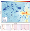 |
Fig. 1 Ratio of the strength of the FUV radiation field and volume density (G0/n) in Orion B, and the distribution of pixels in dense and translucent gas. Top panel: G0/n at 40 arcseconds (0.08 pc at the distance of the source) across Orion B, where G0 is in Habing's units and n in units of cm−3. Black contour corresponds to 13CO integrated intensity of 0.5 K km s−1, indicating the boundaries of a GMC. Dashed contours correspond to values of G0/n of 1 cm3 (orange) and 20 cm3 (dark red). We divide Orion B in six different regions. The bottom panels show histograms of normalized distribution of pixels having specific dust extinction (left panel), mean volume density (middle panel) and G0/n (right panel). The orange and purple shaded regions correspond to values of pixels from translucent and dense medium, respectively. |
2.2 Intensities
We computed the integrated intensity (W - moment 0) maps for the set of molecular lines used in this work, with their main properties shown in Table 1. First, we created a mask in the position-position-velocity cube to reduce the impact of the noise, following the method presented in Einig et al. (2023). We produce such a signal-to-noise (S/N) mask for each molecule. The mask includes contiguous 3-dimensional regions with a S/N of the peak brightness of at least 2. After masking the data cube, we collapsed the velocity axis along a specific velocity window (last column in Table 1) to ensure all the emission along the line of sight is captured. For computing the W values of molecules that do not show a hyperfine structure (or where the hyperfine structure is not resolved, as in the case of HNC) the integration window is fixed to the same velocity range as for 13CO. However, in the case of HCN, N2H+, C2H and CN (which have a hyperfine structure labeled with “h” in Table 1), resulting in the detection of individual components of the multiplet, we modified the velocity window to ensure that we have taken into account all the detected emission. We did not consider the presence of multiple velocity components (Gaudel et al. 2023; Bešlić et al. 2024), or the existence of different gas layers along the line of sight (Ségal et al. 2024), which could be found in certain regions. Instead, we included the intensity of all the velocity components in our model.
Computing the integrated intensity of lines with a hyperfine structure requires an additional step, namely, computing the intensity of the multiplet components used in analysis in B21. For instance, B 21 did not consider the hyperfine splitting of HCN and N2H+, and we integrated the emission of all hyperfine components along the line of sight. For the remaining two molecules (C2H. and CN), the hyperfine structure was taken into account. B21 used the intensity of the C2H line at 87.328 GHz, and the brightest component of the CN multiplet at 113.490 GHz. To properly measure the intensity of these specific components, we used the information on relative intensities of the components of the multiplets of C2H and CN (Table A.1). We first computed the total intensities of C2H and CN and then multiplied these by factors of 0.135 and 0.5, respectively. With this approach, we computed the intensities of C2H(3/2,1 → 1/2,0) and CN(5/2 → 3/2) used in B21, ensuring the minimization of the impact of the noise in the spectrum of these lines and possible cases when the components or the multiplet are blended.
Finally, to compute the column density ratios of CN/N2H+and C2H/HNC (hereafter, N(CN)/N(N2H+)and N(C2H)/N(HNC)), respectively-we assumed a local thermodynamic equilibrium (LTE) and an optically thin regime where the column density is linearly proportional to the measured line intensity. When computing column densities, we assumed the same excitation temperature of Tex=9.375 K for all species. These calculations are described in detail in Appendix B.
Properties of the observed molecular lines used in this work.
2.3 Visual extinction, volume density and incident radiation field
Throughout this work, we used available maps of key parameters describing the interstellar gas across Orion B, such as the maps of visual extinction Av (Fig. C.1), the mean mass-weighted volume density (n) and incident radiation field G0 (previously presented in Santa-Maria et al. 2023). The visual extinction is derived from dust maps obtained by Herschel and presented in Lombardi et al. (2014). We used the Av map to define regions of translucent and dense gas (regions within the orange and purple contours in Fig. C.1) across Orion B, assuming that Av is a good tracer of the H2 column density (Planck Collaboration XI 2014).
The volume density maps of Orion B are derived from column density maps and shown in Orkisz & Kainulainen (2025). These maps are a production of key properties from the probability density function (PDF) of volume density in each pixel, for instance, the mean volume density and the peak density. Here, we use the information on the mean volume density normalized by mass, assuming fully isotropic and unfragmented cloud. We compared Av and n across Orion B to ensure that regions with high n correspond to regions with high visual extinction, and we show this comparison in Fig. C.2.
The strength of the radiation field G0, is computed based on the spectral energy distribution (SED) fits to the farinfrared/submillimeter (FIR/submm) emission of dust grains heated by the interstellar radiation field (Santa-Maria et al. 2023). Throughout this study, we investigated how the ionization fraction changes with the volume density, and mainly how it changes with the G0/n, which controls much of the physics and chemistry in the PDR gas (Sternberg et al. 2014). We show a map of G0/n in the top panel of Fig. 1.
2.4 Model predictions for the ionization fraction and selection of lines
In the top panel of Fig. 1, we show the boundaries of the Orion B GMC with a black contour, defined using 13CO(1−0) intensity detected across the region (Figure 1 in Pety et al. 2017), corresponding to a W(13CO(1−0)) of 0.5 K km s−1. Within this region, Av spans a range from 0.7 mag to over 200 mag. Following the models defined in B21, we compute the ionization fraction in two types of environments in Orion B. These areas are defined based on the visual extinction: translucent (2 mag ≤ Av ≤ 6 mag) and dense (Av ≥ 10 mag) medium. By taking into account only the pixels within the black contour in the top panel of Fig. 1, we find that 16% of them correspond to the diffuse medium (Av<2 mag), 74% of them are in the translucent medium (2 mag ≤ Av ≤ 6 mag), and 3% of pixels are in the dense regions (Av ≥ 10 mag). The remaining percentage (7%) corresponds to a region between 6 magAv<10 mag, which we did not analyze in this work because this range of Av contains gas that is still impacted by far-ultraviolet (FUV) radiation on the cloud; therefore, it does not represent the dense and shielded medium. In addition, we did not investigate the diffuse medium, since the ionization fraction in this region is expected to reach the values that one would derive from the relative carbon abundance (fe ≍ 10−4). Overall, we computed the ionization fraction across a large portion (77%) of Orion B.
The parametrization of the ionization fraction as a function of the line ratio (x) is given by a polynomial function (B21), expressed as
 (2)
where
(2)
where
 (3)
(3)
The FUV radiation field heavily drives the chemistry in the translucent gas, whereas the dense gas becomes shielded against FUV radiation while becoming sensitive to cosmic rays. We note that the model of dense gas in B21 does not consider the stellar UV radiation field and the analytical formula for dense gas is only valid for G0=1.
In the bottom panels of Figure 1, we show the distribution of visual extinction (left panel), mass-weighted volume density (middle panel), and G0/n on the right panel. The distribution is shown for all pixels having W(13CO(1−0))>0.5 K km s−1. In these histograms, we show the ranges of Av, n, and G0/n that are found in both translucent and dense gas. The bottom-left panel of Fig. 1 shows the criteria we use to define translucent and dense gas regions. In the case of n and G0/n, the dense medium shows larger dynamical ranges of n and G0 than the translucent gas. The translucent medium has a range of volume densities of (60−1 · 104 cm−3) with a median value of 110 cm−3, whereas the range of volume densities in dense gas spans from 6.5 · 102 to 5 · 105 cm−3 with the median volume density of 3 · 103 cm−3. In the translucent gas, G0/n shows a range from 8 · 10−4 to 31 cm3, and in the dense medium, a range of 4 · 10−4−30 cm3.
The coefficients defined in Equation (2) for both media and the respective line intensity and column density ratios used in this work are given in Tables 2 and B.2. In the work of B21, over 66 and 91 different line ratios (intensity and column densities for the translucent and dense medium, respectively) were used to probe the ionization fraction. Here, we use the recommended line ratios in each medium to derive fe. This selection was based on the sensitivity of molecular lines to electrons and the coefficient R2 that measures the accuracy of the regression model to predict the ionization fraction (see, e.g., Table B6 in B21) and therefore the quality of the tracer (line intensity or column density ratio). In addition to this criterion, we also considered the detectability of molecular lines and focus on those typically used in galactic and extragalactic studies. In particular, we chose to use the integrated intensity ratio and column density ratio of CN/N2H+for the dense medium. In addition to CN/N2H+, we also use 13CO/HCO+and C18O/HCO+to derive fe in dense gas. For the translucent medium, we use the intensity and column density ratios of C2H/HNC, and will comment on the ionization fraction derived from the C2H/HCN and C2H/CN intensity ratios.
Parameters for the model predicted ionization fraction in dense and translucent gas from B21.
3 Results: Dense gas
All pixels satisfying the condition Av ≥ 10 mag are considered to belong to the dense medium shown within the purple contours in Fig. C.1. For clarity, we split the dense gas into a few regions shown in the top panel of Fig. 1: NGC 2024, the Cloak, B9, the Hummingbird filament, the Horsehead nebula, and the dense region between the Horsehead Nebula and NGC 2023. Each has different properties in terms of external radiation field and gas density. As seen from the top panel of Fig. 1, these dense regions within Orion B are differently exposed to stellar feedback, which we will also discuss here, given the fact that models of dense gas in B 21 did not consider the impact of external radiation fields.
B21 recommended the W(CN)/W(N2H+)ratio as the best tracer of the ionization fraction in dense gas. On one hand, CN is a typical tracer of PDRs, sensitive to UV radiation and often observed around young stars (Pety et al. 2017). CN is also an important actor of nitrogen chemistry in dense and cold cores (Hily-Blant et al. 2013). On the other hand, N2H+is a typical tracer of dense and cold regions formed in the reaction between N2 and  and it is destroyed by recombination with electrons and reactions with CO.
3.1 Ionization fraction from the CN(1-0)/N2H+(1-0) line intensity ratio
First, we show the variation of fe computed from W(CN)/W(N2H+)with the volume density in Fig. 2. Each point represents one pixel from our map whose intensity ratio falls within the validity range defined by models in B21 (Appendix D). In total, around 95% of CN/N2H+pixels (the fraction of the dense medium pixels where CN and N2H+are detected) fall in the corresponding validity range (Fig. D.1). The gray contours show the density of points. In addition, we binned the observed trend by region and volume density. These binned trends are shown in different colors for each region. The error bar of each binned point represents the measured uncertainties of points within each bin and also reflects the spread of the values.
The majority of data points have the ionization fraction around 10−6 (the dark grey region in Fig. 2). We observe that the ionization fraction varies by region, and that fe decreases with increasing volume density of the gas. The computed ionization fraction in dense gas spans from 10−5.5 in the lower-density regions (n ≈ 103 cm−3), and decreases toward the densest parts of Orion B, where it reaches values between 10−7.5 and 10−6.5. The highest fe is present in NGC 2024, whereas the lowest fe has been found in sightlines towards the Hummingbird and B 9.
Such a relationship between the ionization fraction and the volume density is expected from chemical models since the dense regions are more shielded against UV radiation, and recombination is more effective at high densities. Consequently, the emission of a UV-sensitive molecule, such as CN in this case, will become faint, while the emission of the density-sensitive molecule (N2H+in this case) will increase, which will lower the W(CN)/W(N2H+)ratio and, therefore, also lower the observed ionization fraction (top panel in Fig. D.1).
We further quantified the relation between the ionization fraction and volume density. First, we bin all data points by volume density, excluding NGC 2024 region, because this region shows strong UV radiation. We discuss the implications of this later in this paper. These are shown in Fig. 3. Then, we fit the linear model (log (fe)=a · log(n) + b) to the binned values. Because we show and investigate the logarithmic values of ionization fraction and volume density in Fig. 3, the linear relation in log space corresponds to a power-law in linear space. We followed the prescription of such a linear regression from Ségal et al. (2024). The fit is shown in purple in Fig. 3. The measured slope is −0.227 ± 0.003 and the intercept is −5.29 ± 0.06.
Next, we show our results on the ionization fraction computed using W(CN)/W(N2H+)as a function of the strength of the radiation field derived by the mass density-weighted mean volume density in Fig. 4. In this figure, G0/n (and G0) increases to the right. Consequently, pixels showing moderate to high G0/n (yellow and red pixels in the top panel of Fig. 1), also display the highest ionization fractions, whereas data points with low G0/n have moderate to low ionization fractions.
This result suggests that, besides the gas density, G0 has an impact on the computed ionization fraction of Orion B, which is especially notable in regions of intense radiation field, in the West of Orion B, such as NGC 2024. To investigate the impact of the local environment on fe, we separately analyze pixels based on their location: B9, the Cloak, the Hummingbird, NGC 2024, NGC 2023 and the Horsehead nebula. As seen in the top panel of Figs. 1 and C.1, these regions span a wide range in G0/n space, which makes it important to consider their properties when interpreting the fe. To do so, similarly as in Fig. 2, we bin data points within each region by G0/n, and include these binned trends in Fig. 4. The pixels in the Horsehead nebula show the lowest range of G0/n, whereas the broadest range in G0/n is found in NGC 2024 (almost four orders of magnitude). Here we also find that fe depends on the specific region being analyzed and that regions with stronger G0 have higher fe.
All regions shown in Fig. 4 have fe values between 10−7.5 and 10−5.5. The highest ionization fraction is found across NGC 2024 (up to fe of 10−5.5), the region containing the densest gas and the strongest radiation field in our map. The ionization fraction of NGC 2023, the Horsehead, and the Hummingbird is similar (taking values from 10−6.5 and 10−5.75), whereas the lowest ionization fraction is found in B9 (∼10−7.5). Different fe values in these regions can be explained by taking into account their characteristics. For instance, B9 hosts cold, dense cores and displays low G0/n values: whereas NGC 2024 is a place of active star formation, with present strong UV radiation. The Horsehead nebula is an edge-on PDR, and NGC 2023 is a reflection nebula surrounded by cold and dense gas.
From Fig. 4, it is notable that the fe depends on local properties; specifically, the gas density and radiation field. This is especially evident in NGC 2024, where G0/n reaches the highest values of G0/n, and where we see the strongest variation of fe. A strong radiation field can yield a stronger and deeper impact on the cloud, which can then enhance the emission of UV-sensitive molecules such as CN and HCO+(Gratier et al. 2017; Bron et al. 2018), and contributes to the increased number of ionizations. This interpretation can possibly explain the difference in binned trends between regions of low and high G0, as shown in Fig. 4. However, as the gas becomes denser, the ionization fraction is expected to decrease since recombination reactions become more effective in the denser gas. We will further discuss our findings in the context of gas shielding and other impacts on observed line emission in the upcoming sections.
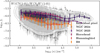 |
Fig. 2 Ionization fraction computed using the W(CN)/W(N2H+)ratio as a function of volume-weighted mean volume density, n. Contours correspond to the density of points of 1, 5, 25, 50, and 75 percent (from the most outer to the most inner contour). Colored dots are the binned trends of pixels from the different regions in Orion B (top panel of Fig. 1). The error bars show the weighted standard deviation of the points within each bin. |
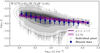 |
Fig. 3 Same as Fig. 2, but showing the binned trend of all data points except for the NGC 2024 region. The purple line shows the linear fit and its uncertainty. |
Tabulated median values of the ionization fraction across different regions in Orion B: NGC 2024, NGC 2023, the Horsehead nebula, the Hummingbird filament, B9 and the Cloak.
3.2 Ionization fraction from 13CO(1-0)/HCO+(1-0) and C18O(1-0)/HCO+(1-0) intensity ratios
We present results on fe in dense gas computed using W(13CO)/W(HCO+)and W(C18O)/W(HCO+). Optically thin CO isotopologs trace the cloud interior, particularly C18O (Ségal et al. 2024). HCO+has a high critical density (see Table 1) and is, similarly to CN, it is sensitive to UV radiation and present in PDRs (Gratier et al. 2017; Hernández-Vera et al. 2023). HCO+ can trace the inner structure of clouds, as it can be formed in reactions initiated by cosmic rays (Gaches et al. 2019). In addition, these lines have good S/N and are spatially extended across Orion B (Pety et al. 2017).
We show fe derived from W(13CO)/W(HCO+)and W(C18O)/W(HCO+)as a function of G0/n in Figs. F.1 and F.2. Similarly to the case of W(CN)/W(N2H+), we have observed that G0/n impacts fe derived from W(13CO)/W(HCO+)and W(C18O)/W(HCO+). To compare these findings, we show results on the ionization fraction computed using these three line intensity ratios for each region (reflecting different regimes of G0 as well, Sect. 3.1) in Fig. 5. We note here that 13CO, C18O, and HCO+are also detected across the Cloak, which contains pixels with the lowest G0/n (around 2 cm3) across Orion B.
We present median values of the ionization fraction derived from three line intensity ratios for each region considered as dense gas in Table 3. The median value of the ionization fraction depends on the tracer and varies across regions. In particular, we note that the ionization fraction decreases with G0/n. We observe variations of fe across each region computed from each line intensity and as a function of G0/n. The highest ionization fraction is derived from W(CN)/W(N2H+)in all regions except B9, and the lowest fe in dense gas in found when using W(C18O)/W(HCO+)as a tracer. We also note the spread in values of fe computed from these three line ratios. It seems that in regions with high G0, such as NGC 2024, NGC 2023, the Horsehead, and even the Hummingbird, we observe a large spread in fe, up to two orders of magnitude.
In the bottom left panel of Fig. 5, (i.e., the case of NGC 2024), we see that fe strongly depends on the selection of a tracer. For instance, the fe derived from W(CN)/W(N2H+)is increasing with G0/n, whereas we observe the opposite behavior from the remaining two line ratios. A similar behavior is observed in the Hummingbird filament (top left panel in Fig. 5). In the case of NGC 2023 and the Horsehead nebula (bottom middle and right panels in Fig. 5), fe derived using all three line ratios behaves the same way with G0/n. The results on fe are highly consistent for the case of B9 and the Cloak (top middle and right panels in Fig. 5) and do not depend on the choice of the line ratio. In these two regions, the ionization fraction increases with G0/n, ranging from 10−7.5 to 10−6. The slight difference between our results on fe seen across B9 and the Cloak is because the properties of these regions are closest to the model hypotheses presented in B21. In the case of B9, the spread in fe is larger than the uncertainties of these trends. We continue our discussion on the observed trends in Sect. 6.
4 Results: Translucent gas
Translucent regions in Orion B are shown within the orange contours in Fig. C.1. To compute the ionization fraction of translucent gas, we used integrated intensity ratios of molecules sensitive to FUV radiation, such as C2H and CN and those whose emission scales with the column density: HNC and HCN.
As one of the simplest hydrocarbons, C2H shows enhanced abundances in PDR gas (Pety et al. 2005; Beuther et al. 2008; Cuadrado et al. 2015; Goicoechea et al. 2025). The production of C2H depends on the presence of C+, one of the source of electrons in the interstellar medium (ISM), which makes this molecule a good choice for probing the fe in translucent gas. The production paths of HCN and HNC are coupled, and electrons are essential for their excitation in a translucent region (Santa-Maria et al. 2023). At least 50% of total HCN and HNC emission across Orion B is found in translucent gas (Santa-Maria et al. 2023). While HNC has an unresolved hyperfine structure, and its profile can be described using a single Gaussian function, the hyperfine structure of HCN(1−0) is resolved in three separate hyperfine components. However, in most of the ORION-B field of view, the hyperfine components of HCN exhibit anomalous excitation (Goicoechea et al. 2022; Santa-Maria et al. 2023), an effect not taken into account in B21 radiative transfer calculations, and which requires sophisticated calculations for deriving the HCN column density. Therefore, we chose to primarily focus on the analysis of fe derived from the ratio of C2H and HNC (intensity and column density), and in the rest of this section, we compare our findings with those computed from W(C2H)/W(HCN) and W(C2H)/W(CN).
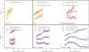 |
Fig. 5 Ionization fraction in dense gas derived from intensity ratios of CN and N2H+,13CO and HCO+and C18O and HCO+as a function of G0/n in six dense regions in Orion B. We show binned trends by G0/n, and the errorbars correspond to the 25 th and 75 th percentiles. |
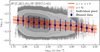 |
Fig. 6 Ionization fraction computed from W(C2H)/W(HNC) as a function of n in translucent gas. Similarly as in Fig. 2, we show the scatter of data points and the gray contours correspond to the density of data points. The binned trends are shown in dark blue. The error bars are computed in the same way as in Fig. 2. |
4.1 The ionization fraction from the intensity ratio C2H(1-0)/HNC(1-0)
We present results of fe in the translucent medium computed using W(C2H)/W(HNC) as a function of n and G0/n in Figs. 6 and 7 respectively. The density of data points is shown by grey contours, as in Fig. 2. In both figures, the binned trend is shown in dark blue color. We find that the ionization fraction in translucent gas ranges between 10−5.5 and 10−4, which is higher than the ionization fraction found in dense gas (Sect. 3). The highest ionization fraction (≈ 10−4.5) is found in the low-density regions (n ≈ 102−102.5 cm−3) in translucent gas (Fig. 6). The fe decreases by 0.5 dex toward higher volume densities, where it reaches ≈ 10−5.25. These values of fe found in translucent gas in Orion B are between the typical values of fe for the atomic ISM and for molecular regions where carbon is fully ionized (10−4) and the typical fe found in translucent gas (6 · 10−5., Snow & McCall 2006).
In translucent conditions, it is expected that the ionization fraction decreases with increasing volume density. Such relation is described via power-law function, where: fe ∝ n−1/2 (McKee 1989; Caselli et al. 1998). Similarly as in dense gas, we fit a linear function to log10 fe−log10 n, and show the result in orange in Fig. 6. We derive a slope of −0.3 ± 0.02 and an intercept of −4.32 ± 0.14.
The majority of pixels in Fig. 7 have the lowest values of G0/n(<1 cm3) and are found in the entire map (Fig. 1), while the pixels with G0/n greater than 1 cm3 are found in NGC 2024 and the Horsehead nebula. Here, we observe that the fe increases from ≈10−5.5 to 10−4.5 for G0/n going from 10−3 to 1 cm3, after which fe remains nearly constant. Overall, the higher values of the ionization fraction in translucent gas across Orion B as compared with the dense gas regions suggest that carbon is partially ionized and sulfur could be fully ionized in this low density regime. The translucent regions then correspond to the transition zone from the ionized to the neutral carbon layer of a PDR. We further discuss this in Sect. 5.4.
Tabulated median values of the ionization fraction in translucent gas using intensity ratios of W(C2H)/W(HNC), W(C2H)/W(HCN), and W(C2H)/W(CN).
4.2 The ionization fraction in translucent gas derived from C2H(1−0)/HCN(1−0) and C2H(1−0)/CN(1−0)
We present our results on fe values computed from W(C2H)/W(HCN) and W(C2H)/W(CN) in the translucent medium. The corresponding fe as a function of G0/n is shown in Figs. G.1 and G.2. By using W(C2H)/W(HCN) and W(C2H)/W(CN) to trace fe in translucent gas, we find that the value of the ionization fraction does not significantly vary depending on the tracer. The median fe derived from these three line ratios is shown in Table 4. We find that the median fe ranges from 10−4.75 to 10−4.5. The lowest fe, is derived using W(C2H)/W(HNC), while the highest ionization fraction is calculated from W(C2H)/W(CN). The highest scatter in fe, is observed when using W(C2H)/W(HCN), as a tracer (Fig. G.1), where we also observe that several lines of sight reach values of 10−3.87, which is the saturation value defined by a coefficient fmax in Eq. (2), i.e., the fractional abundance of carbon relative to the total hydrogen content (1.32 · 10−4).
5 Discussion
5.1 Line intensity ratios versus column density ratios
Ionization fraction derived from the column density ratios for both mediums is presented in Appendix E. Here, we compare results on fe derived from intensity and column density ratios (using the same molecular species) and justify our choice of using the line intensity ratio to compute the ionization fraction in Orion B. In B21, models of fe, derived from line intensity ratios are computed from chemical models and single-slab RADEX (van der Tak et al. 2007) models. These assumed uniform gas density, temperature, and electron abundance. Figs. E.1 and E.2 show how the ionization fraction computed from the column density ratios of CN/ N2H+and C2H/HNC in dense and translucent gas, respectively, changes with the G0/n.
In dense gas, when using column density ratios to compute the fe, we find that the ionization fraction also increases with the G0/n, as it is seen when using the intensity ratios of the same species (Fig. 4). The errors of data points are notably smaller than in the case of fe derived from the intensity ratios, because of smaller model uncertainties (first two panels in Fig. D.1). In this case, the fe ranges from 10−7.5 in regions of low G0/n, and goes up to 10−5.5 in NGC 2024 and the Hummingbird. In the translucent medium, the fe derived from N(C2H)/N(HNC) does not vary with G0/n, and the median value is ∼10−4.5.
Our results are consistent between the fe derived from intensity and column density ratios. However, we chose to use the intensity ratios as tracers of the ionization fraction, because they can be directly derived from observations. In contrast, column densities are not directly observable, and their estimation from the observed line intensities requires assumptions on the physical conditions under which the lines are produced. In this case, we derive column densities from the observed line intensities assuming optically thin line emission and the LTE at a fixed excitation temperature for all considered species. The assumption of LTE is valid for the dense regime, whereas it needs to be revisited for the translucent regime. It is important to recognize that the observed molecular lines, despite their critical densities (listed in Table 1 and of an order of magnitude of 104−105 cm−3) can still be produced below the critical density. Processes such as radiative trapping, where the line emission becomes optically thick, can reduce the effective critical density. Considering these effects, it may be more relevant to examine the effective critical density of these species, which accounts for such factors (Shirley 2015). For the lines analyzed in our study, the effective critical density is nearly two orders of magnitude lower than the conventional critical density (the density at which collisions dominate over radiative processes) reported in Table 1. Additionally, it is crucial to consider collisions with electrons, as they are the primary contributors to the excitation of molecules such as HCN and HNC at moderate densities (Santa-Maria et al. 2023).
5.2 The ionization fraction in dense gas
The main ionization processes in dense molecular interstellar gas are related to cosmic rays, with additional more localized contributions from shocks created by protostars or supernovae. Cosmic rays ionize molecular hydrogen producing  , which in reaction with molecular hydrogen gives
  , a molecular ion responsible for the production of several molecular ions, such as HCO+and N2H+(Dalgarno 2006) through reactions with neutral molecular and atomic species, enabling an active ion-molecule gas-phase chemistry in dense shielded gas. In addition to the presence of low ionization potential species, such as sulfur and carbon, the presence of PAHs is also crucial in understanding and determining the ionization fraction, since PAH ions are formed in a straightforward manner via radiative attachment and are likely to carry most of the electric charge.
In dense regions, we derive the ionization fraction using W(CN)/W(N2H+), W(13CO)/W(HCO+), and W(C18O)/W(HCO+). We find that typical values of the ionization fraction somewhat depend on the selected line ratio. General values of the ionization fraction in dense gas computed in this work range from 10−8 to 10−6, which are higher than the values (5 · 10−9−10−7) reported in the literature for a cold dense core (e.g., Goicoechea et al. 2009). This difference comes from different regions probed and the different approaches to computing the ionization fraction. For instance, the value of 5 · 10−9 reported in Goicoechea et al. (2009) is found in a cold and dense, shielded core bright in DCO+, whereas in our case, Orion B contains several dense PDRs (dense regions impacted by strong UV radiation – NGC 2024, NGC 2023, the Horsehead, the Hummingbird). These regions contain dense gas, but they lie close to young stars that affect the surrounding medium. Moreover, B9 and the Cloak are farther from the sources of UV radiation than the regions mentioned above, and we discuss fe, which we found in these regions in the context of their properties.
We find a general dependence on the volume density, but the G0 in dense gas as well, as presented in Sect. 3. That is why we observe a positive correlation between fe and G0/n. Our binning analysis revealed that different environments in Orion B have different ionization fractions, which is expected because these regions show different properties. For instance, regions located in the west of Orion B that are closest to the ζ Orionis star (Alnitak) have enhanced G0/n, driven by a strong radiation field. In addition to this, NGC 2024 shows the strongest star formation in the entire Orion B cloud. The CN emission, tracing the UV-illuminated gas (Gratier et al. 2017; Bron et al. 2018) is bright in these regions.
It is important to note that the dense gas models presented in B21 do not consider variations of G0, whereas the variation with the cosmic ray ionization is acknowledged. In that regard, dense regions with strong external UV radiation studied in this work do not fully correspond to the models from B21, and therefore these results on fe should be treated with caution and as an upper limit. In the case of W(CN)/W(N2H+), as shown in Fig. D.1, our W(CN)/W(N2H+)measurements populate the central and right part of the validity range of the model of B21, missing a domain with a low W(CN)/W(N2H+), line ratio that yields low fe. In dense regions illuminated by strong FUV radiation, bright CN, emission could be produced on the cloud surface, while N2H+ originates from inner parts of dense gas. Therefore, such regions would have a higher W(CN)/W(N2H+), ratio than predicted by dense and shielded gas models, hence a higher value of the derived fe, using B21 models.
5.3 Ionization fraction as a local parameter in dense gas
According to Hollenbach (1990), the value of G0/n controls the structure of a PDR: in regions where G0/n is lower than 10−2 cm3, the self-shielding of H2 is the dominant effect balancing photodissociation, while dust shielding becomes increasingly important for higher values of G0/n. Regions with G0/n above 0.1 cm3 undergo a switch in the regime of the H/H2 transition; whereas in regions with highest G0/n (above 10 cm3), the radiation pressure supersonically drives dust through the gas.
As previously discussed, fe depends on the local properties of the gas. Therefore, we consider and compute the ionization fraction in several regions across Orion B, which are considered as dense medium. There are six regions in total in Orion B that host dense molecular gas (sorted from the easternmost of Alnitak): the Cloak, B9, the Hummingbird, NGC 2024, NGC 2023, and the Horsehead nebula. Each of these regions has different properties in terms of the range of densities, G0, structure and prestellar and protostellar cores, and can be divided into two categories: dense regions with low G0 (the Cloak, B9, and the Hummingbird) and dense PDRs (NGC 2024, NGC 2023, and the Horsehead). In the case of the Cloak, we did not detect any significant CN and N2H+emission in this region. Below, we discuss the results on fe derived from other tracers used in this work in the next section.
B9: this region has low G0 (see Table 3), and shows the narrowest range in volume densities. Previous studies have shown that B9 hosts prestellar and protostellar cores (Miettinen et al. 2010, 2012) characterized by a dynamical evolution. It is an example of an isolated low-mass star-forming region. Nevertheless, the formation of cores in B9 is probably influenced by nearby stars, as this region exhibits multiple velocity components observed in CO emission and its isotopologs (Gaudel et al. 2023). We derived relatively low fe values in B9, of ∼3 · 10−7 with a scatter of a factor of 3.
The Hummingbird: this filament is gravitationally stable (Orkisz et al. 2019) and, interestingly, it does not contain any YSOs, although some condensation and cores have been detected as peaks of C18O emission. Here, fe shows a clear decreasing trend with increasing density in this filament. Overall fe remains moderate but higher than in B 9, ∼5 · 10−7 with a scatter of a factor of 3.
NGC 2023: NGC 2023 is a reflection nebula, and here we also include the dense region nearby, which explains variations in fe across this area. In particular, we found a decreasing trend of fe with increasing density and relatively low values of the ionization fraction in the coldest and densest ridge near to NGC 2023, similar to those found in B9. The median fe value is higher in NGC 2023 than in the previous regions, reaching about 7 · 10−7.
NGC 2024: this is probably one of the most interesting regions of the entire Orion B cloud since it exhibits the most active star formation. In this case, we observe the largest variation in G0/n and in fe. This is because NGC 2024 has a very specific structure: it is composed of an HII region, sorrounded by a dense PDR and the cold dusty filament (the Flame) located in front of the HII region. Moreover, NGC 2024 hosts several protostellar cores, one of which drives a molecular outflow. The Flame filament is on the other hand cold and also a place of star formation. This structure of NGC 2024 can explain our results on fe reported in this work; for instance, we found lower fe values along the Flame filament (∼4 · 10−7), while higher values of the ionization fraction (∼2 · 10−6) are seen in regions of warm dust heated by stellar radiation.
The Horsehead nebula: Goicoechea et al. (2009) found a gradient of the ionization fraction in this region by investigating H13CO+and DCO+. The Horsehead nebula is an edge-on PDR, with a nearby cold dense core. The median value is intermediate between B9 and NGC 2023 and close to that of the Hummingbird filament, about 5 · 10−7.
5.4 Ionization fraction in translucent medium
In the translucent medium, fe takes values from 10−5.5 to 10−4.5 derived from W(C2H)/W(HNC) (Fig. 6), values between 10−5.75 and 10−3.87 when computed from W(C2H)/W(HCN) (Fig. G.1), and 10−5.5 to 10−4.25 when traced by W(C2H)/W(CN) (Fig. G.2). In general, the results on fe in translucent gas computed in this work are consistent among the different tracers. The median fe derived in the translucent gas from these three line intensity ratios, ∼2 · 10−5, varies by less than a factor of 2, and reaches a factor of 4, including the 25th and 75th percentiles (Table 4).
The range of values of the ionization fraction in translucent gas implies that the line emission analyzed in this work is produced in the C+/CI/CO layer, where ionized sulfur is an important contributor of electrons and carbon remains partially ionized (Goicoechea & Cuadrado 2021). These conditions are consistent with the definition of translucent gas presented in Snow & McCall (2006), in which some amount of carbon is ionized. That is why the expected ionization fraction in the translucent gas have values on the order of tenths of a percent of the fractional abundance of carbon (i.e., values between 10−5 and 10−4). Gerin et al. (2024) showed that the ionization fraction is very important for the excitation of the 4.8 GHz line of o-H2CO. This line can have an excitation temperature lower than the (CMB) and be detected in absorption against the CMB for some specific conditions, and gets thermalized with the CMB for ionization fractions approaching 10−4. Widespread absorption associated with extended 13CO emission is seen in translucent gas, which implies moderate values of the ionization fractions, as those independently derived in this work.
In addition, neutral carbon is detected throughout Orion B (bottom-right panel of Fig. 1 in Santa-Maria et al. 2023; Ikeda et al. 2002), as well as emission from CO and 13CO (Pety et al. 2017). Since the Einstein coefficient of the [CI] fine structure line is low, the detected [CII] emission originates from relatively high column densities of neutral carbon, comparable to those of CO. Ikeda et al. (2002) found that atomic carbon represents between 10 and 20 percent of all gas-phase carbon in Orion B.
Furthermore, the high fe values (≥ 10−5) found in lowdensity and high G0/n regions in Orion B imply that the rotational level excitation of some molecules such as HCN and HNC (Goldsmith & Kauffmann 2017; Goicoechea et al. 2022; Santa-Maria et al. 2023) is affected by collisions with electrons in the low-density gas. HCN and HNC 1−0 emissions are present in low- Av gas; Santa-Maria et al. (2023) found that approximately 70% of the total HCN emission comes from Av ≤ 8 mag and a correlation with the Cı emission. The photochemical models in Santa-Maria et al. (2023) yielded an ionization fraction of at least 10−5 in the translucent gas, sufficient for electron excitation to be efficient for HCN and HNC.
6 Caveats
We further discuss our results in this section, with possible implications with respect to the models presented in B21 and results obtained in this work. Our results provide a certain range of the ionization fraction in dense and translucent gas. In both cases, we select tracers recommended in the work of B21. However, it is important to keep in mind the caveats of the models presented in B21 and their limitations. In addition, it is also important to further discuss the complexity of emission in Orion B, and the molecular lines used in this work, including their sensitivity to environmental conditions such as gas density and stellar radiation.
6.1 Model limitations and future improvements
As previously stated, the models presented in B21 do not consider changes with G0 in dense gas. These models describe a dense gas region as a piece of gas shielded from the UV photons, where certain molecular species (such as N2H+) are formed. However, Orion B contains certain regions, especially those on its western side, that are both dense and highly affected by the UV field from young stars. Such specific conditions should be considered in future works, especially for the analysis of emission lines sensitive to FUV radiation.
6.2 The reliability of tracers of fe in Orion B
6.2.1 Dense medium
Here, we focus on discussing fe derived from a set of different intensity ratios in dense gas. To interpret our results, we have to consider that each of these molecular lines are differently sensitive to gas conditions such as density and temperature. Our results (Fig. 5) show that the highest ionization fraction is derived when using intensity ratio of W(CN)/W(N2H+), while the smallest fe is derived from W(C18O)/W(HCO+). In regions with low G0/n, such as B9 and the Cloak, the ionization fraction shows the smallest variation among pixels and varies by less than 0.6 dex between the different tracers, whereas in NGC 2024 for example, the variation in fe depending on the choice of the tracer is up to 1.5 dex. This result is supported by the fact that lines used to derive fe in dense gas are not equally sensitive to G0 and the gas density which in turn will impact the estimated ionization fraction. For example, CN and HCO+will contain a significant contribution from PDRs, while C18O and N2H+only trace the dense and shielded gas. The line ratio W(CN)/W(N2H+) has a dense gas tracer in the denominator (the ratio of a line sensitive to UV/density-sensitive line), whereas in the case of W(13CO)/W(HCO+)and W(C18O)/W(HCO+)the denominator is a PDR tracer (i.e., vice versa). This means that in regions where CN and HCO+get bright due to enhanced UV radiation, one line ratio will increase, while the other one will become lower.
Such a finding has a few implications. The first one is that we can trust our results in regions of low G0/n, especially in the Cloak, B9, and the lowest G0/n regions of the Hummingbird, because the fe derived from different tracers are overall consistent within less than 1 dex. The difference arises as we move towards high G0/n regions because molecules sensitive to the intense UV field will have enhanced emission, increasing (lowering) the W(CN)/W(N2H+)(W(C18O)/W(HCO+))ratio. In such regions, CN and HCO+become overbright and may come primarily from the surface of the cloud, whereas molecules such as N2H+and C18O arise from the inner parts of the molecular cloud.
Another aspect that could help in the interpretation of our results lies in the following. Lines of sight in Orion B are the superposition of multiple features (layers), associated with different velocity components in the spectrum of these molecular lines, most notably in CO isotopologs (Gaudel et al. 2023), although Bešlić et al. (2024) found up to three velocity components in CN and HCO+emission in NGC 2024. Furthermore, the observed spectrum of each molecular line is the result of radiative interaction of gas in multiple layers along the line of sight, such as dense cores and more diffuse medium. Such complex structures were not accounted for in the simple chemical models used in B21. In this case, each molecule will differently trace such layers, and as a consequence, these layers will differently contribute to the total molecular emission (Ségal et al. 2024). By considering this scenario, it is probable that, for instance, in the case of W(C18O)/W(HCO+), these two emission lines originate from and probe somewhat different gas layers, as shown in the case of the Horsehead nebula by Ségal et al. (2024). Similarly, in the case of W(CN)/W(N2H+), although CN is observed toward the entire NGC 2024 region, it could be mainly tracing UV-heated gas, whereas N2H+is present in the cold and dense part.
Moreover, it is important to acknowledge the effect of opacity, in which case, the corresponding line emission can originate from the surface of a cloud, instead of probing the full line of sight. On the one hand, 13CO gets optically thick, and therefore its emission can trace only the outer parts of molecular clouds. Similarly, CN and HCO+emission can also get saturated (as in the case of NGC 2024, Bešlić et al. 2024), but at higher densities than 13CO. On the other hand, C18O is known to be a good tracer of inner parts of molecular gas (Pety et al. 2017), although it can be depleted in cold gas.
Considering all the discussion points given above, we provide a recommendation on the choice of the tracer of ionization fraction in dense gas. In all cases, we recommend the choice of molecular lines which approximately probe the same gas, where one of them is sensitive to the FUV radiation. In the case of regions with low G0/n (from 10−3 cm3 to 2 · 10−2 cm3), we recommend using any of these three tracers, since fe derived from these three line ratios nicely agree. In the case of regions with high G0/n (from 2 · 10−2 cm3), we recommend to use fe derived from W(CN)/W(N2H+)as an upper limit, and values of fe derived from W(C18O)/W(HCO+)as a lower limit.
In addition, it is important to bear in mind that fe found in this work is derived from the total emission along the line of sight and provides a general overview of the ionization fraction across Orion B. This means, as explained in Sect. 2, that we did not treat individual components of molecular emission coming from different velocity layers or distinguish between diffuse and dense gas along the line of sight (e.g., filament versus envelope). At the moment, this type of analysis is beyond the scope of this work, but we plan to address this issue in future studies.
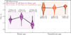 |
Fig. 8 The distribution of the ionization fraction in dense medium computed from line ratios of 13CO/HCO+, CN/N2H+and C18O/HCO+(left part of the figure, purple shaded area). In the right part of this figure, we show results on fe derived from W(C2H)/W(HCN), W(C2H)/W(HNC), W(C2H)/W(CN) in translucent medium (orange shaded area). Black dashed violins show distributions of all pixels that have detection in the corresponding intensity ratio. Purple violins show pixels only from regions where CN/N2H+is detected, whereas orange violins show the same for W(C2H)/W(HNC). We also show the median for each of these categories as a horizontal line. |
6.2.2 Translucent medium
Regarding the translucent gas, our results did not significantly vary based on the selection of a tracer, mainly since the excitation by electrons becomes important for HCN, HNC and CN. However, given the overlap with the validity range and resolved hyperfine structures of HCN and CN, including the anomalous excitation of HCN, we recommend the use of W(C2H)/W(HNC) for estimating the ionization fraction.
6.2.3 The impact of pixel selection criteria on the ionization fraction
Finally, we comment on fe computed from three different line ratios for both dense and translucent gas by considering the pixel selection effect. First, we consider the dense medium. The overall fe derived from W(CN)/W(N2H+)is different from that inferred from W(13CO)/W(HCO+)or from W(C18O)/W(HCO+) for chemical reasons as discussed above, and also because the sensitivity threshold for detecting these lines can also impact our results. Therefore, we compare the distribution of the ionization fraction derived from W(CN)/W(N2H+), W(13CO)/W(HCO+), and W(C18O)/W(HCO+)in the left part of Fig. 8. In the same figure, we show the distribution of fe from these line ratios obtained by taking into account exactly the same pixels from the map. fe from W(CN)/W(N2H+)contains the lowest number of pixels, indicating that regions where both lines are detected probe the densest parts of Orion B in comparison to W(13CO)/W(HCO+)and W(C18O)/W(HCO+). When we observe fe from the same pixels, we see that the median fe from W(13CO)/W(HCO+)and W(C18O)/W(HCO+)is lower than in the case of taking into account all data points. This finding implies that W(CN)/W(N2H+)probes the densest parts of Orion B, whereas W(13CO)/W(HCO+)and W(C18O)/W(HCO+) are more spatially distributed, containing lower density pixels, that have a higher ionization fraction.
7 Summary
In this study, we measured the ionization fraction across almost the entire Orion B giant molecular cloud using IRAM 30-meter observations from the ORION B large program and analytical models to predict the ionization fraction from line intensity or column density ratios presented in Bron et al. (2021). We show the map of ionization fraction in Fig. 9. In the context of Orion B, we analyzed the ionization fraction in translucent (2 ≤ mag Av ≤ 6 mag) and dense gas (Av ≥ 10 mag). We investigated its variations with the strength of the incident FUV radiation characterized by G0 and with the volume density n. Following the models and recommendations from Bron et al. (2021), we used the following tracers ((1−0) transitions) of the ionization fraction:
In dense gas, we used the intensity and column density ratios of CN and N2H+, and the intensity ratios of 13CO and HCO+and of C18O and HCO+.
In translucent regions, we computed fe using intensity and column density ratios of C2H and HNC, and intensity ratios of C2H and HCN and C2H and CN.
Our key findings in the dense medium are:
The ionization fraction in dense gas is in the range from 10−7.75 to 10−6.5.
We find that the ionization fraction slightly decreases with increasing volume density, with a power-law slope of −0.227.
When using W(CN)/W(N2H+)to compute fe, we find that regions with strong FUV field show higher ionization fraction than regions with low G0. We do not observe any such dependence on G0 when using the two other intensity ratios.
Our results on ionization fraction in the dense medium are consistent when using different intensity ratios in regions of weak FUV radiation (B9, the Cloak, the Hummingbird, parts of NGC 2023), whereas in NGC 2024 and the Horsehead nebula the range of values of ionization fraction varies by an order of magnitude.
These results can be understood considering the sensitivity of CN and HCO+to the UV radiation. In dense regions irradiated by strong UV radiation, CN and HCO+emission may result from the surface layers of FUV-illuminated clouds, whereas the N2H+and C18O emission comes from the inner part of the clouds.
The key results in translucent gas are:
The ionization fraction in translucent medium is found between 10−5.5 and 10−4.
Similarly to dense medium, we not observe a variation of fe with n, with a somewhat steeper power-law slope of −0.3.
fe derived from W(C2H)/W(HNC), W(C2H)/W(HCN), and W(C2H)/W(CN) are consistent within the uncertainties.
The values of the ionization fraction found in this medium suggest that the molecular gas considered as translucent lies in the transition layer from ionized carbon to atomic carbon to CO, and where excitation with electrons becomes an important aspect of the excitation of HCN, HNC and CN rotational line emission.
Considering all the above, we find the ionization fraction in the range of (10−7.75, 10−6.5) in dense gas and in the range of (10−5.5, 10−4) in translucent medium across Orion B. We suggest using results derived from W(CN)/W(N2H+)as an upper limit of the ionization fraction, along with W(C18O)/W(HCO+)as a lower limit to the ionization fraction in dense gas. In terms of the translucent gas, we recommend using the intensity ratio that mostly overlaps with the model validity range, which in our case is W(C2H)/W(HNC).
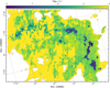 |
Fig. 9 Map of ionization fraction across Orion B. We show the fe at 120 arcseconds (0.24 pc) derived using W(C2H)/W(HNC) in translucent gas and in regions of Av between 6 mag and 10 mag, and W(C18O)/W(HCO+)in dense gas. In diffuse medium (Av<2) and in region where we do not detect any W(C2H)/W(HNC), we set the ionization fraction to be 10−4. The black contours show the boundaries of Orion B, defined from W(13CO(1−0)) emission. |
Acknowledgements
We thank the anonymous referee for useful comments that have improved the manuscript. This work is based on observations carried out under project numbers 019-13, 022-14, 145-14, 122-15, 018-16, and finally the large program number 124-16 with the IRAM 30 m telescope. IRAM is supported by INSU/CNRS (France), MPG (Germany) and IGN (Spain). This work received support from the French Agence Nationale de la Recherche through the DAOISM grant ANR-21-CE31-0010, and from the Programme National “Physique et Chimie du Milieu Interstellaire” (PCMI) of CNRS/INSU with INC/INP, co-funded by CEA and CNES. M.G.S.M. and J.R.G. thank the Spanish MICINN for funding support under grant PID2023-146667NB-I00. M.G.S.M acknowledges support from the NSF under grant CAREER 2142300. Part of the research was carried out at the Jet Propulsion Laboratory, California Institute of Technology, under a contract with the National Aeronautics and Space Administration (80NM0018D0004). D.C.L. acknowledges financial support from the National Aeronautics and Space Administration (NASA) Astrophysics Data Analysis Program (ADAP).
Appendix A Hyperfine structure of C N(1 − 0) and C2 H(1 − 0)
In Table A.1, we list information about the hyperfine structure of CN(1−0) and C2H(1−0). The properties of CN(1−0) are taken from Savage et al. (2002), while the information for C2H(1−0) is from Padovani et al. (2009). The transition of CN(1−0) is divided into two groups, each containing a multiplet of five hyperfine components. The brighter group is observed at ∼113.5 GHz, while the second one can be observed at 113.12 GHz. Our observations specifically cover the brighter group of CN(1−0) hyperfine multiplet, in which we detect four out of the five components (the first four rows related to CN(1−0) in Table A.1). On the other hand, C2H(1−0) consists of six hyperfine components. Our data set includes two of these components, 3/2, 2 → 1/2, 1, and 3/2, 1 → 1/2, 0.
Properties of the hyperfine splitting of CN(1−0) and C2H(1−0).
Appendix B Column densities
Assuming the LTE case and that our lines are optically thin (opacity, τ ≪ 1), the column density of the upper state u of the considered molecular transition scales linearly with the integrated intensity: Nu= const · W. The full expression is as follows:
![Mathematical equation: $N_{\mathrm{u}}\left[\mathrm{cm}^{-2}\right]=1.9436 \cdot 10^{7} \frac{v}{A_{\mathrm{ul}}} \cdot\left[1-\frac{e^{\left(4.8 \cdot v \cdot T_{\mathrm{ex}}\right)}-1}{e^{\left(4.8 \cdot v \cdot T_{\mathrm{CMB}}\right)}-1}\right]^{-1} \cdot W.$](/articles/aa/full_html/2025/10/aa53706-25/aa53706-25-eq26.png) (B.1)
In the above equation, v is the frequency of the transition in units of 100 GHz, Aul is the Einstein coefficient of the transition in s −1, Tex is the excitation temperature in K, and TCMB is the temperature of the cosmic microwave background emission of 2.73 K. The total column density is then computed as:
(B.1)
In the above equation, v is the frequency of the transition in units of 100 GHz, Aul is the Einstein coefficient of the transition in s −1, Tex is the excitation temperature in K, and TCMB is the temperature of the cosmic microwave background emission of 2.73 K. The total column density is then computed as:
 (B.2)
where Q(Tex) is the partition function computed for excitation temperature Tex, gu is the degeneracy of the upper level, Eu is the upper level energy, and kB is the Boltzmann's constant.
(B.2)
where Q(Tex) is the partition function computed for excitation temperature Tex, gu is the degeneracy of the upper level, Eu is the upper level energy, and kB is the Boltzmann's constant.
Table B.1 summarizes the parameters needed for computing the column densities of the corresponding species considered in this work. Einstein coefficients, the upper level energy, the degeneracy, and the partition function are taken from The Cologne Database for Molecular Spectroscopy (CDMS; Müller et al. 2001, 2005; Endres et al. 2016). Assuming that the emission of these lines is subthermally excited (Roueff et al. 2021; Ségal et al. 2024), we take the excitation temperature to 9.375 K for this work.
Assuming the excitation temperature is the same for both species, in cases where we are not in the LTE regime, their column density ratio is almost independent of the choice of excitation temperature. We find that the column density ratio in this case is changed by less than 10 percent from the one measured assuming the LTE case with the excitation temperature equal to the dust temperature. In the nonLTE case, assuming that the excitation temperature is different for each species for which we compute the column density ratio, we find that the column density ratio can change by up to 100 percent, but that in most of the cases the variation is less than 20 percent. Nevertheless, given the variation of fe with respect to the column density ratios in Figs. D.1 and D.2, this difference does not introduce significant uncertainties in our measurements. We note, however, that appropriate measurements of column densities of the species analyzed in our work will be the topic of future studies.
Parameters of selected molecules and J=1−0 transitions.
Appendix C Visual extinction as a tracer of volume density in Orion B
We used the map of the dust visual extinction, Av from Lombardi et al. (2014), shown in Fig. C.1, to define regions of dense and translucent molecular gas in Orion B. In this figure, translucent and dense gas regions are found within the orange and purple contours, respectively. Since we are investigating how the ionization fraction varies as a function of G0 and volume density n, we explore the relationship between Av and n. For further information on the derivation of volume density maps of Orion B, we direct the reader to Orkisz & Kainulainen (2025). In Fig. C.2 we present the mean mass density-weighted volume density (Orkisz & Kainulainen 2025) as a function of visual extinction with points color-coded by their G0 values. The observed scatter indicates a positive correlation between Av and n.
Appendix D Models and validity ranges
D.1 Dense medium
Figure D.1 shows the ionization fraction computed for dense medium by applying Eq. 2 and using coefficients from Table 2. In all panels, the black line represents analytical function (Eq. 2), and the grey shaded area shows its 3−σ variance. Purple horizontal line corresponds to the validity range derived from models in B21. The validity range is defined as the range of values in intensity and column density ratios within which the analytical formulae (Eq. 2) are valid (the uncertainty falls below 2%). The blue horizontal line represents the range in values derived from our observations. The first row shows fe derived from CN/N2H+(intensity and column density ratios), while the bottom row shows fe computed using W(13CO)/W(HCO+)and W(C18O)/W(HCO+).
Parameters for the model predicted ionization fraction in dense and translucent gas from B21 derived using column density of molecular lines.
 |
Fig. C.1 Dust visual extinction across Orion B. This map was derived from dust column density (Lombardi et al. 2014). Orange contours show regions of translucent gas, where Av is in the range from 2 mag to 6 mag. Purple contours show regions of dense gas. |
The largest overlap with the validity range is observed for the intensity ratio of 13CO/HCO+(bottom right panel), where we see that the entire validity range was covered in our measurements. Next is the CN/N2H+intensity ratio (top left panel), where the overlap spans three orders of magnitude. Our observations did not cover values of W(CN)/W(N2H+)lower than 10−1.8. In addition, only a few lines of sight have an observed W(CN)/W(N2H+)higher than the maximum value provided from the validity range. Interestingly, our measurements cover a lower part of the validity range for the column density ratio of CN and N2H+The log of W(13CO)/W(HCO+)and log of W(C18O)/W(HCO+)range from −0.25 to 2.25 and −1 to 1.25, respectively. These ranges fall within the validity range for both line ratios, which is somewhat wider, especially on the left side.
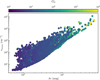 |
Fig. C.2 Mean mass density-weighted volume density as a function of visual magnitude. We color-code each point by a corresponding strength of radiation field (G0). |
Percentage of pixels of each intensity ratio in the model validity range of B21.
In Table D.1 we show the percentages of pixels for each molecular ratio used in this work that fall within the validity range (Bron et al. 2021). For each ratio considered in dense gas, we observe that most pixels (more than 90 percent) fall within this validity range.
D.2 Translucent medium
For the case of translucent gas, we show fe as a function of line ratios in Fig. D.1. C2H/HNC intensity ratio derived from observations shows the largest range compared with other line ratios considered in this work, and it takes values in the validity range. The observed C2H/HCN takes the lower values of the validity range. In the case of C2H/CN, this line ratio shows the smallest overlap with the validity range, as well as N(C2H)/N(HNC).
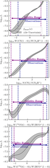 |
Fig. D.1 Ionization fraction as a function of selected line intensity ratios for dense gas. The range of observed line ratios is shown in blue and the validity range is in purple. We show the analytical function as a black solid line showing relation between fe (y-axis) and intensity ratios (x-axis) of CN/N2H+(top panel), N(CN)/N(N2H+)(second panel), 13CO/HCO+(third panel), and C18O/HCO+(bottom panel). The analytical functions (Eq. 2), its 3−σ variance (grey shaded area) and the validity ranges are taken from Bron et al. (2021). |
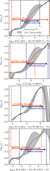 |
Fig. D.2 Same as in D.1, but in the case of translucent gas. Here, we show fe as a function of intensity ratios of C2H/HNC (top panel), column density ratio of C2H/HNC (second panel), C2H/HCN (third panel), and C2H/CN (bottom panel). |
Appendix E Ionization fraction computed from column density ratios
E.1 The ionization fraction in dense gas from the column density ratio of CN/N2H+
We present our results on fe in dense gas computed from column density ratios of CN and N2H+. We emphasize that we use a different approach to compute column densities than the one used in B21, where column densities were determined from the chemical models. After the column densities are derived, we use Eq. 2 and the corresponding coefficients from Table B.2 to compute fe. All of N(CN)/N(N2H+)pixels fall within the validity range (see the second panel in Fig. D.1) defined in B21.
We show our results on the ionization fraction derived from the column density ratio of CN and N2H+as a function of G0/n in Fig. E.1. As shown in Sect. 3.1 and Fig. 4, we show here binned trends of the ionization fraction of each region. Using a column density ratio as a tracer of the ionization fraction, we find similar values of fe than those derived using the intensity ratio of the same molecular species. These results imply that our assumption of the LTE and optically thin emission to compute column densities is valid in the dense gas in Orion B. The scatter in Fig. E.1 is smaller than in the case of fe computed from intensity ratios. The ionization fraction changes from 10−7.2 to 10−5.5, and increases toward regions with high G0/n. The lowest ionization fraction is found in low G0/n parts of the Hummingbird and across B9, whereas the highest fe is found across NGC 2024.
E.2 Ionization fraction from the column density ratio of C2H(1−0)/HNC(1−0)
The ionization fraction computed from the column density ratio of C2H and HNC as a function of G0/n is presented in Fig. E.2. The observed column density ratio falls more in the right part of the validity range than the W(C2H)/W(HNC), so the predictions of fe from N(C2H)/N(HNC) extend to higher fe values. Nevertheless, the median ionization fraction in translucent gas derived from column density ratios is 10−4.5, consistent with the values derived in Sect. 4.1.
Appendix F lonization fraction in dense gas using W(1 C C)/W(HCO+)and W(C18O)/W(HCO+)
Moreover, we present measurements of the ionization fraction of Orion B in dense gas (Sect. 3) using 13CO/HCO+and C18O/HCO+as tracers in Figs. F.1 and F.2 respectively. Similarly, as in Fig. 4, we show binned trends of each region. In comparison to fe derived from W(CN)/W(N2H+), we here also detect the target lines in the Cloak region, whose binned trends are shown in yellow.
In both these cases, dense regions showing lower radiation field strength, B9 and the Cloak, have the highest ionization fraction (∼10−6.5 to 10−6 from W(13CO)/W(HCO+), and ∼10−7 to 10−6.5 from.W(C18O)/W(HCO+)), whereas high-UV illuminated regions show lower ionization fraction, among which the lowest fe is measured toward NGC 2023 and NGC 2024. This supports our conclusion that the line intensity ratios involving HCO+can be biased in regions exposed to intense FUV radiation and provide only a lower limit to the ionization fraction, as already discussed in Sect. 5.2.
Appendix G Ionization fraction in translucent gas using W(C2H)/W(HCN) and W(C2H)/W(CN)
We show results on the ionization fraction computed from W(C2H)/W(HCN) and W(C2H)/W(CN) for translucent gas (Sect. 4) and corresponding binned trends as a function of G0/n in Figs. G.1 and G.2. We do not observe significant variation in fe derived from these two line ratios with G0/n.
References
- Basu, S., & Mouschovias, T. C., 1994, ApJ, 432, 720 [NASA ADS] [CrossRef] [Google Scholar]
- Bergin, E. A., Plume, R., Williams, J. P., & Myers, P. C., 1999, ApJ, 512, 724 [NASA ADS] [CrossRef] [Google Scholar]
- Beuther, H., Semenov, D., Henning, T., & Linz, H., 2008, ApJ, 675, L33 [Google Scholar]
- Bešlić, I., Coudé, S., Lis, D. C., et al. 2024, A&A, 684, A212 [NASA ADS] [CrossRef] [EDP Sciences] [Google Scholar]
- Bik, A., Lenorzer, A., Kaper, L., et al. 2003, A&A, 404, 249 [NASA ADS] [CrossRef] [EDP Sciences] [Google Scholar]
- Bron, E., Daudon, C., Pety, J., et al. 2018, A&A, 610, A12 [CrossRef] [EDP Sciences] [PubMed] [Google Scholar]
- Bron, E., Roueff, E., Gerin, M., et al. 2021, A&A, 645, A28 [NASA ADS] [CrossRef] [EDP Sciences] [Google Scholar]
- Cao, Z., Jiang, B., Zhao, H., & Sun, M., 2023, ApJ, 945, 132 [NASA ADS] [CrossRef] [Google Scholar]
- Caselli, P., Walmsley, C. M., Terzieva, R., & Herbst, E., 1998, ApJ, 499, 234 [Google Scholar]
- Caselli, P., Walmsley, C. M., Zucconi, A., et al. 2002, ApJ, 565, 344 [Google Scholar]
- Ceccarelli, C., Codella, C., Balucani, N., et al. 2023, ASP Conf. Ser., 534, 379 [NASA ADS] [Google Scholar]
- Cuadrado, S., Goicoechea, J. R., Pilleri, P., et al. 2015, A&A, 575, A82 [NASA ADS] [CrossRef] [EDP Sciences] [Google Scholar]
- Cuadrado, S., Salas, P., Goicoechea, J. R., et al. 2019, A&A, 625, L3 [NASA ADS] [CrossRef] [EDP Sciences] [Google Scholar]
- Dalgarno, A., 2006, Proc. Natl. Acad. Sci., 103, 12269 [Google Scholar]
- Dalgarno, A., & Lepp, S., 1984, ApJ, 287, L47 [NASA ADS] [CrossRef] [Google Scholar]
- Draine, B. T., 2011, Physics of the Interstellar and Intergalactic Medium (Berlin: Springer) [Google Scholar]
- Einig, L., Pety, J., Roueff, A., et al. 2023, A&A, 677, A158 [NASA ADS] [CrossRef] [EDP Sciences] [Google Scholar]
- Endres, C. P., Schlemmer, S., Schilke, P., Stutzki, J., & Müller, H. S. P., 2016, J. Mol. Spectr., 327, 95 [Google Scholar]
- Fuente, A., Cernicharo, J., Roueff, E., et al. 2016, A&A, 593, A94 [NASA ADS] [CrossRef] [EDP Sciences] [Google Scholar]
- Gaches, B. A. L., Offner, S. S. R., & Bisbas, T. G., 2019, ApJ, 883, 190 [NASA ADS] [CrossRef] [Google Scholar]
- Gaudel, M., Orkisz, J. H., Gerin, M., et al. 2023, A&A, 670, A59 [NASA ADS] [CrossRef] [EDP Sciences] [Google Scholar]
- Gerin, M., Liszt, H., Pety, J., & Faure, A., 2024, A&A, 686, A49 [NASA ADS] [CrossRef] [EDP Sciences] [Google Scholar]
- Goicoechea, J. R., & Cuadrado, S., 2021, A&A, 647, L7 [NASA ADS] [CrossRef] [EDP Sciences] [Google Scholar]
- Goicoechea, J. R., Pety, J., Gerin, M., Hily-Blant, P., & Le Bourlot, J., 2009, A&A, 498, 771 [NASA ADS] [CrossRef] [EDP Sciences] [Google Scholar]
- Goicoechea, J. R., Lique, F., & Santa-Maria, M. G., 2022, A&A, 658, A28 [NASA ADS] [CrossRef] [EDP Sciences] [Google Scholar]
- Goicoechea, J. R., Pety, J., Cuadrado, S., et al. 2025, A&A, 696, A100 [NASA ADS] [CrossRef] [EDP Sciences] [Google Scholar]
- Goldsmith, P. F., 2001, ApJ, 557, 736 [Google Scholar]
- Goldsmith, P. F., & Kauffmann, J., 2017, ApJ, 841, 25 [Google Scholar]
- Gratier, P., Bron, E., Gerin, M., et al. 2017, A&A, 599, A100 [CrossRef] [EDP Sciences] [Google Scholar]
- Guelin, M., Langer, W. D., Snell, R. L., & Wootten, H. A., 1977, ApJ, 217, L165 [NASA ADS] [CrossRef] [Google Scholar]
- Guelin, M., Langer, W. D., & Wilson, R. W., 1982, A&A, 107, 107 [NASA ADS] [Google Scholar]
- Herbst, E., & Klemperer, W., 1973, ApJ, 185, 505 [Google Scholar]
- Hernández-Vera, C., Guzmán, V. V., Goicoechea, J. R., et al. 2023, A&A, 677, A152 [NASA ADS] [CrossRef] [EDP Sciences] [Google Scholar]
- Hily-Blant, P., Pineau des Forêts, G., Faure, A., Le Gal, R., & Padovani, M. 2013, A&A, 557, A65 [NASA ADS] [CrossRef] [EDP Sciences] [Google Scholar]
- Hollenbach, D. J., 1990, ASP Conf. Ser., 12, 167 [Google Scholar]
- Ikeda, M., Oka, T., Tatematsu, K., Sekimoto, Y., & Yamamoto, S., 2002, ApJS, 139, 467 [NASA ADS] [CrossRef] [Google Scholar]
- Lombardi, M., Bouy, H., Alves, J., & Lada, C. J., 2014, A&A, 566, A45 [NASA ADS] [CrossRef] [EDP Sciences] [Google Scholar]
- Maret, S., & Bergin, E. A., 2007, ApJ, 664, 956 [Google Scholar]
- McKee, C. F., 1989, ApJ, 345, 782 [NASA ADS] [CrossRef] [Google Scholar]
- Miettinen, O., Harju, J., Haikala, L. K., & Juvela, M., 2010, A&A, 524, A91 [NASA ADS] [CrossRef] [EDP Sciences] [Google Scholar]
- Miettinen, O., Hennemann, M., & Linz, H., 2011, A&A, 534, A134 [NASA ADS] [CrossRef] [EDP Sciences] [Google Scholar]
- Miettinen, O., Harju, J., Haikala, L. K., & Juvela, M., 2012, A&A, 538, A137 [NASA ADS] [CrossRef] [EDP Sciences] [Google Scholar]
- Müller, H. S. P., Thorwirth, S., Roth, D. A., & Winnewisser, G., 2001, A&A, 370, L49 [Google Scholar]
- Müller, H. S. P., Schlöder, F., Stutzki, J., & Winnewisser, G., 2005, J. Mol. Struc., 742, 215 [Google Scholar]
- Oppenheimer, M., & Dalgarno, A., 1974, ApJ, 192, 29 [NASA ADS] [CrossRef] [Google Scholar]
- Orkisz, J. H., & Kainulainen, J., 2025, A&A, 697, A20 [NASA ADS] [CrossRef] [EDP Sciences] [Google Scholar]
- Orkisz, J. H., Peretto, N., Pety, J., et al. 2019, A&A, 624, A113 [NASA ADS] [CrossRef] [EDP Sciences] [Google Scholar]
- Pabst, C. H. M., Goicoechea, J. R., Cuadrado, S., et al. 2024, A&A, 688, A7 [NASA ADS] [CrossRef] [EDP Sciences] [Google Scholar]
- Padovani, M., Walmsley, C. M., Tafalla, M., Galli, D., & Müller, H. S. P., 2009, A&A, 505, 1199 [NASA ADS] [CrossRef] [EDP Sciences] [Google Scholar]
- Padovani, M., Hennebelle, P., & Galli, D., 2013, A&A, 560, A114 [NASA ADS] [CrossRef] [EDP Sciences] [Google Scholar]
- Pattle, K., Fissel, L., Tahani, M., Liu, T., & Ntormousi, E., 2023, ASP Conf. Ser., 534, 193 [NASA ADS] [Google Scholar]
- Pety, J., Teyssier, D., Fossé, D., et al. 2005, A&A, 435, 885 [NASA ADS] [CrossRef] [EDP Sciences] [Google Scholar]
- Pety, J., Guzmán, V. V., Orkisz, J. H., et al. 2017, A&A, 599, A98 [NASA ADS] [CrossRef] [EDP Sciences] [Google Scholar]
- Planck Collaboration XI., 2014, A&A, 571, A11 [NASA ADS] [CrossRef] [EDP Sciences] [Google Scholar]
- Redaelli, E., Bovino, S., Lupi, A., et al. 2024, A&A, 685, A67 [NASA ADS] [CrossRef] [EDP Sciences] [Google Scholar]
- Roueff, E., Loison, J. C., & Hickson, K. M., 2015, A&A, 576, A99 [NASA ADS] [CrossRef] [EDP Sciences] [Google Scholar]
- Roueff, A., Gerin, M., Gratier, P., et al. 2021, A&A, 645, A26 [NASA ADS] [CrossRef] [EDP Sciences] [Google Scholar]
- Salas, P., Rugel, M. R., Emig, K. L., et al. 2021, A&A, 653, A102 [NASA ADS] [CrossRef] [EDP Sciences] [Google Scholar]
- Santa-Maria, M. G., Goicoechea, J. R., Pety, J., et al. 2023, A&A, 679, A4 [NASA ADS] [CrossRef] [EDP Sciences] [Google Scholar]
- Savage, C., Apponi, A. J., Ziurys, L. M., & Wyckoff, S., 2002, ApJ, 578, 211 [NASA ADS] [CrossRef] [Google Scholar]
- Ségal, L., Roueff, A., Pety, J., et al. 2024, A&A, 692, A160 [NASA ADS] [CrossRef] [EDP Sciences] [Google Scholar]
- Shingledecker, C. N., Bergner, J. B., Le Gal, R., et al. 2016, ApJ, 830, 151 [NASA ADS] [CrossRef] [Google Scholar]
- Shirley, Y. L., 2015, PASP, 127, 299 [Google Scholar]
- Snow, T. P., & McCall, B. J., 2006, ARA&A, 44, 367 [NASA ADS] [CrossRef] [Google Scholar]
- Sternberg, A., Le Petit, F., Roueff, E., & Le Bourlot, J., 2014, ApJ, 790, 10 [CrossRef] [Google Scholar]
- van der Tak, F. F. S., Black, J. H., Schöier, F. L., Jansen, D. J., & van Dishoeck, E. F., 2007, A&A, 468, 627 [NASA ADS] [CrossRef] [EDP Sciences] [Google Scholar]
- Williams, J. P., Bergin, E. A., Caselli, P., Myers, P. C., & Plume, R., 1998, ApJ, 503, 689 [NASA ADS] [CrossRef] [Google Scholar]
- Zakardjian, A., Hughes, A., Pety, J., et al. 2025, A&A, 696, A165 [NASA ADS] [CrossRef] [EDP Sciences] [Google Scholar]
All Tables
Parameters for the model predicted ionization fraction in dense and translucent gas from B21.
Tabulated median values of the ionization fraction across different regions in Orion B: NGC 2024, NGC 2023, the Horsehead nebula, the Hummingbird filament, B9 and the Cloak.
Tabulated median values of the ionization fraction in translucent gas using intensity ratios of W(C2H)/W(HNC), W(C2H)/W(HCN), and W(C2H)/W(CN).
Parameters for the model predicted ionization fraction in dense and translucent gas from B21 derived using column density of molecular lines.
Percentage of pixels of each intensity ratio in the model validity range of B21.
All Figures
|
Fig. 1 Ratio of the strength of the FUV radiation field and volume density (G0/n) in Orion B, and the distribution of pixels in dense and translucent gas. Top panel: G0/n at 40 arcseconds (0.08 pc at the distance of the source) across Orion B, where G0 is in Habing's units and n in units of cm−3. Black contour corresponds to 13CO integrated intensity of 0.5 K km s−1, indicating the boundaries of a GMC. Dashed contours correspond to values of G0/n of 1 cm3 (orange) and 20 cm3 (dark red). We divide Orion B in six different regions. The bottom panels show histograms of normalized distribution of pixels having specific dust extinction (left panel), mean volume density (middle panel) and G0/n (right panel). The orange and purple shaded regions correspond to values of pixels from translucent and dense medium, respectively. |
| In the text | |
|
Fig. 2 Ionization fraction computed using the W(CN)/W(N2H+)ratio as a function of volume-weighted mean volume density, n. Contours correspond to the density of points of 1, 5, 25, 50, and 75 percent (from the most outer to the most inner contour). Colored dots are the binned trends of pixels from the different regions in Orion B (top panel of Fig. 1). The error bars show the weighted standard deviation of the points within each bin. |
| In the text | |
|
Fig. 3 Same as Fig. 2, but showing the binned trend of all data points except for the NGC 2024 region. The purple line shows the linear fit and its uncertainty. |
| In the text | |
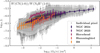 |
Fig. 4 Same as Fig. 2, but fe is shown as a function of G0/n. |
| In the text | |
|
Fig. 5 Ionization fraction in dense gas derived from intensity ratios of CN and N2H+,13CO and HCO+and C18O and HCO+as a function of G0/n in six dense regions in Orion B. We show binned trends by G0/n, and the errorbars correspond to the 25 th and 75 th percentiles. |
| In the text | |
|
Fig. 6 Ionization fraction computed from W(C2H)/W(HNC) as a function of n in translucent gas. Similarly as in Fig. 2, we show the scatter of data points and the gray contours correspond to the density of data points. The binned trends are shown in dark blue. The error bars are computed in the same way as in Fig. 2. |
| In the text | |
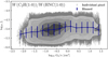 |
Fig. 7 Same as Fig. 6, but for G0/n. |
| In the text | |
|
Fig. 8 The distribution of the ionization fraction in dense medium computed from line ratios of 13CO/HCO+, CN/N2H+and C18O/HCO+(left part of the figure, purple shaded area). In the right part of this figure, we show results on fe derived from W(C2H)/W(HCN), W(C2H)/W(HNC), W(C2H)/W(CN) in translucent medium (orange shaded area). Black dashed violins show distributions of all pixels that have detection in the corresponding intensity ratio. Purple violins show pixels only from regions where CN/N2H+is detected, whereas orange violins show the same for W(C2H)/W(HNC). We also show the median for each of these categories as a horizontal line. |
| In the text | |
|
Fig. 9 Map of ionization fraction across Orion B. We show the fe at 120 arcseconds (0.24 pc) derived using W(C2H)/W(HNC) in translucent gas and in regions of Av between 6 mag and 10 mag, and W(C18O)/W(HCO+)in dense gas. In diffuse medium (Av<2) and in region where we do not detect any W(C2H)/W(HNC), we set the ionization fraction to be 10−4. The black contours show the boundaries of Orion B, defined from W(13CO(1−0)) emission. |
| In the text | |
|
Fig. C.1 Dust visual extinction across Orion B. This map was derived from dust column density (Lombardi et al. 2014). Orange contours show regions of translucent gas, where Av is in the range from 2 mag to 6 mag. Purple contours show regions of dense gas. |
| In the text | |
|
Fig. C.2 Mean mass density-weighted volume density as a function of visual magnitude. We color-code each point by a corresponding strength of radiation field (G0). |
| In the text | |
|
Fig. D.1 Ionization fraction as a function of selected line intensity ratios for dense gas. The range of observed line ratios is shown in blue and the validity range is in purple. We show the analytical function as a black solid line showing relation between fe (y-axis) and intensity ratios (x-axis) of CN/N2H+(top panel), N(CN)/N(N2H+)(second panel), 13CO/HCO+(third panel), and C18O/HCO+(bottom panel). The analytical functions (Eq. 2), its 3−σ variance (grey shaded area) and the validity ranges are taken from Bron et al. (2021). |
| In the text | |
|
Fig. D.2 Same as in D.1, but in the case of translucent gas. Here, we show fe as a function of intensity ratios of C2H/HNC (top panel), column density ratio of C2H/HNC (second panel), C2H/HCN (third panel), and C2H/CN (bottom panel). |
| In the text | |
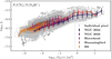 |
Fig. E.1 Same as in Fig. 4, but using N(CN)/N(N2H+)to compute the ionization fraction. |
| In the text | |
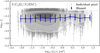 |
Fig. E.2 Same as in Fig. 6, but we show fe computed from the column density ratio of W(C2H)/W(HNC). |
| In the text | |
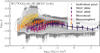 |
Fig. F.1 Same as Fig. 4, but for W(13CO)/W(HCO+). |
| In the text | |
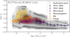 |
Fig. F.2 Same as Fig. 4, but for W(C18O)/W(HCO+). |
| In the text | |
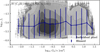 |
Fig. G.1 Same as Fig. 7, but showing scatter of fe computed from W(C2H)/W(HCN). |
| In the text | |
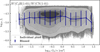 |
Fig. G.2 Same as Fig. 7, but for fe inferred from W(C2H)/W(CN). |
| In the text | |
Current usage metrics show cumulative count of Article Views (full-text article views including HTML views, PDF and ePub downloads, according to the available data) and Abstracts Views on Vision4Press platform.
Data correspond to usage on the plateform after 2015. The current usage metrics is available 48-96 hours after online publication and is updated daily on week days.
Initial download of the metrics may take a while.