| Issue |
A&A
Volume 702, October 2025
|
|
|---|---|---|
| Article Number | A23 | |
| Number of page(s) | 19 | |
| Section | Interstellar and circumstellar matter | |
| DOI | https://doi.org/10.1051/0004-6361/202554035 | |
| Published online | 30 September 2025 | |
Analysis of the isotopologues of CS, CCS, CCCS, HCS+, HCCS+, and H2CS in TMC-1 with the QUIJOTE line survey★
1
Dept. de Astrofísica Molecular, Instituto de Física Fundamental (IFF-CSIC),
C/ Serrano 121,
28006
Madrid,
Spain
2
Department of Applied Chemistry, Science Building II, National Yang Ming Chiao Tung University,
1001 Ta-Hsueh Rd.,
Hsinchu
300098,
Taiwan
3
Université de Rennes, CNRS, IPR (Institut de Physique de Rennes) – UMR 6251,
35000
Rennes,
France
4
Observatorio de Yebes (IGN), Cerro de la Palera s/n,
19141
Yebes, Guadalajara,
Spain
5
Observatorio Astronómico Nacional (OAN, IGN),
C/ Alfonso XII, 3,
28014
Madrid,
Spain
★★ Corresponding authors: This email address is being protected from spambots. You need JavaScript enabled to view it.
, This email address is being protected from spambots. You need JavaScript enabled to view it.
Received:
5
February
2025
Accepted:
9
July
2025
Abstract
We performed a detailed analysis of the isotopologues with 13C, 34S, 33S, and 36S of the sulphur-bearing molecules CS, CCS, CCCS, HCS+, HCCS+, and H2CS towards the starless core TMC-1 using the QUIJOTE1 line survey. The observations were obtained with the Yebes 40 m radio telescope, and the sensitivity of the data varied between 0.08 and 0.2 mK in the 31–50 GHz range. Observations with the IRAM 30 m radio telescope of the most abundant isotopologues of these species are also presented and used to estimate volume densities and to constrain the excitation conditions of these molecules. Among these species, we report the first detection in space of C13C34S, CC33S, CCC33S, HC33S+, and HCC34S+. C36S is also detected for the first time in a cold starless object. These data were complemented with sensitive maps that provide the spatial distribution of most of these species. Using the available collisional rate coefficients for each species, we modeled the observed line intensities using the large velocity gradient method for the radiative transfer. The results allowed us to report the most complete analysis of the column densities of the CnS family and to compare the abundance ratios of all detected isotopologues. Adopting a kinetic temperature for TMC-1 of 9 K, we found that n(H2)=0.9–1.5×104 cm−3 can explain the observed decline in intensity with increasing rotational levels J for all observed molecules. We derived the rotational constants for the C13C34S, CC33S, CCC33S, HC33S+, and HCC34S+ isotopologues from new laboratory data and complemented them with the frequencies of the observed lines. We find that all sulphur isotopologues are consistent with solar isotopic abundance ratios. Accurate 12C/13C abundances were derived and, as previously suggested, the 13C isotopologues of CCS and CCCS show strong abundance anomalies depending on the position of the substituted carbon. Nevertheless, the 12C/13C abundance ratio is practically identical to the solar value for CS, HCS+, and H2CS. We also searched for the isotopologues of other S-bearing molecules in the 31–50 GHz domain (HCS, HSC, NCS, H2CCS, HCSCN, HCCCS+, C4S, and C5S). The expected intensities for their 34S and 13C isotopologues are too low to be detected with the present sensitivity of the QUIJOTE line survey, however. The results presented in this work provide new insights into the molecular composition, isotopic abundances, and physical conditions of the cold starless core TMC-1.
Key words: astrochemistry / line: identification / molecular data / ISM: molecules / ISM: individual objects: TMC-1
Based on observations carried out with the Yebes 40 m telescope (projects 19A003, 20A014, 20D023, 21A011, 21D005, 22A007, 22B029 and 23A024) and the Institut de Radioastronomie Millimétrique (IRAM) 30 m telescope. The 40 m radio telescope at Yebes Observatory is operated by the Spanish Geographic Institute (IGN, Ministerio de Transportes y Movilidad Sostenible). IRAM is supported by INSU/CNRS (France), MPG (Germany) and IGN (Spain).
© The Authors 2025
 Open Access article, published by EDP Sciences, under the terms of the Creative Commons Attribution License (https://creativecommons.org/licenses/by/4.0), which permits unrestricted use, distribution, and reproduction in any medium, provided the original work is properly cited.
This article is published in open access under the Subscribe to Open model. This email address is being protected from spambots. You need JavaScript enabled to view it. to support open access publication.
1 Introduction
The cold dark cloud TMC-1 has emerged as a promising laboratory for the detection of a great number of molecules. This cloud has a carbon-rich chemistry that favours the formation of a high variety of molecules with a large unsaturated carbon chain. The recent discoveries made with the QUIJOTE1 line survey of this source carried out with the Yebes 40 m radio telescope (Cernicharo et al. 2021a), has shown an incredible unexpected chemical richness.
Sensitive line surveys are a powerful method with which to search for the chemical complexity of a cloud. The sensitivity reached by QUIJOTE has permitted us to detect nearly 70 new molecules in TMC-1, including cations, anions, radicals, and cycles. As the sensitivity increases, a new issue appears in the interpretation of the data: All isotopologues of the most abundant species were detected in the data. This means that rare species containing D, 13C, 15N, 34S, 33S, and even 36S or double substituted isotopologues, have to be identified in order to avoid possible pitfalls when searching for new molecular species. Many of these isotopologues have been observed in the laboratory, and a search for them is easy. For other isotopologues, however, we lack information on their rotational spectroscopy, and identifying their lines in the survey becomes as exciting as the detection of new species.
The study with QUIJOTE of the isotopologues present in the cloud is currently a work in progress. In recent years, new isotopologues were detected in TMC-1, such as CH2DC3N (Cabezas et al. 2021), CH2DC4H (Cabezas et al. 2022a), singly substituted isotopologues of HCCNC and HNCCC (Cernicharo et al. 2024a), and doubly substituted isotopologues of HC3N (Tercero et al. 2024). The isotopologues of many species were previously studied at different galactocentric distances using different telescopes and sensitivities (see, e.g., Lucas & Liszt 1998; Milam et al. 2005; Sakai et al. 2007, 2013; Yan et al. 2023, and references therein). Together with the observation of a limited number of transitions for each species, this might introduce some biases in the conclusions concerning their abundances. Moreover, the rate coefficients have been shown to be dependent on the isotopologues that are considered (Flower & Lique 2015; Navarro-Almaida et al. 2023).
The most abundant sulphur-bearing species in TMC-1, which allow us to measure the isotopic abundances of sulphur and carbon, belong to the CnS and HCnS+ families. In particular, CS, CCS, and CCCS are among the most abundant molecules in cold dark clouds. The variety of S-bearing molecules is not as vast as those that contain nitrogen or oxygen, however. The abundance and number of sulphur-bearing species is limited, to a large extent, by the significant depletion of sulphur in the cloud (Fuente et al. 2019; Navarro-Almaida et al. 2020; Fuente et al. 2023). In recent years, the models for the chemical composition of TMC-1 have been progressively refined with the discovery of new S-bearing molecules with the QUIJOTE line survey, such as C4S, C5S (previously detected in evolved stars), H2CCS, H2CCCS, HC4S, NCS, HCSCN, HCSCCH, and NCCHCS (Cernicharo et al. 2021d,e; Fuentetaja et al. 2022; Cabezas et al. 2024), HCCS+ (Cabezas et al. 2022b), HCCCS+ (Cernicharo et al. 2021f), HCNS (Cernicharo et al. 2024b), and CH3CHS (Agundez et al. 2025).
In this work, we present an analysis of the isotopologues of CS, CCS, CCCS, HCS+, HCCS+, and H2CS. The high abundance of CS, CCS, and CCCS in TMC-1, combined with the exceptional sensitivity of the QUIJOTE survey, allows us to detect singly and doubly substituted isotopologues. We provide a detailed study of isotopologues that are singly substituted with 33S, 34S, and 13C for these three abundant species, and of C36S and the 13C34S double isotopologue of CS. The lines of the different isotopologues are relatively close in frequency, which allows us to calculate column densities with high quality so that we avoid calibration errors, if there are any. We also derive the chemical fractionation enhancements of the 13C isotopologues of the different species.
New laboratory rotational spectroscopy of CC33S and CCC33S have permitted us to detect these rare isotolopogues for the first time in space. In addition, using the hyperfine constants of C13CS and the substitution structure of CCS derived from the spectroscopic information available for all its singly substituted isotopologues, we have found four lines in our data that we assign to C13C34S. HC33S+ is also identified in our data. Its rotational constants have been derived from the measured line frequencies of seven hyperfine components belonging to its J=1–0 and 2–1 rotational transitions. For the isotopologues of HCCS+, we assign four features of the QUIJOTE data to HCC34S+. Finally, the rotational and hyperfine constants of C13CS have been improved using the frequencies of the transitions observed in this study.
2 Observations
2.1 Line surveys
The observational data we used are part of QUIJOTE1 (Cernicharo et al. 2021a), a spectral line survey of TMC-1 in the Q band carried out with the Yebes 40 m telescope at the position αJ2000 = 4h41m41.9s and δJ2000 = +25°41′27.0″, which corresponds to the cyanopolyyne peak (CP) in TMC-1. The receiver was built within the Nanocosmos project2. A detailed description of the system was given by Tercero et al. (2021).
The data of the QUIJOTE line survey presented here were gathered in several observing runs between November 2019 and July 2023. The measured sensitivity by July 2023 varied between 0.08 mK at 32 GHz and 0.2 mK at 49.5 GHz, and it is better by about 50 times than that of previous line surveys in the Q band of TMC-1 (Kaifu et al. 2004). A detailed description of the QUIJOTE line survey was provided by Cernicharo et al. (2021a).
The main-beam efficiency measured during our observations in 2022 varied from 0.66 at 32.4 GHz to 0.50 at 48.4 GHz (Tercero et al. 2021) and is given across the Q band by Beff = 0.797 exp[−(ν(GHz)/71.1)2]. The forward telescope efficiency is 0.97. The telescope beam size at half-power intensity is 54.4″ at 32.4 GHz and 36.4″ at 48.4 GHz.
The data of TMC-1 taken with the IRAM 30 m telescope consist of a 3 mm line survey that covers the full available band at the telescope, between 71.6 GHz and 117.6 GHz. The data were described by Cernicharo et al. (2012). More recent high-sensitivity observations in 2021 were used to improve the signal-to-noise ratio (S/N) in several frequency windows (Agúndez et al. 2022; Cabezas et al. 2022b; Cernicharo et al. 2024b).
The IRAM 30 m beam varies between 34″ and 21″ at 72 GHz and 117 GHz, respectively, while the beam efficiency takes values of 0.83 and 0.78 at the same frequencies, following the relation Beff = 0.871 exp[−(ν(GHz)/359)2]. The forward efficiency at 3 mm is 0.95.
The intensity scale used in this work for both telescopes, the antenna temperature (![Mathematical equation: $\[T_{A}^{*}\]$](/articles/aa/full_html/2025/10/aa54035-25/aa54035-25-eq1.png) ), was calibrated using two absorbers at different temperatures and the ATM atmospheric transmission model (Cernicharo 1985; Pardo et al. 2001). Calibration uncertainties were adopted to be 10 %. All data were analysed using the GILDAS package3.
), was calibrated using two absorbers at different temperatures and the ATM atmospheric transmission model (Cernicharo 1985; Pardo et al. 2001). Calibration uncertainties were adopted to be 10 %. All data were analysed using the GILDAS package3.
2.2 Maps
The observed emission in a frequency sweep is often modelled with very limited information on its spatial extent. In the QUIJOTE line survey, the only available spatial information is provided by the variation in the telescope half-power beam with the frequency across the line survey. The spatial sizes of the observed molecules, together with the issues related to the line opacities and radiative transfer, can only be addressed through a spatial mapping of the molecular emission. To overcome these issues, the QUIJOTE line survey is being complemented with high-sensitivity maps obtained with the Yebes 40 m and IRAM 30 m radio telescopes. At the 40 m telescope, ~100 hours of observing time have been devoted to cover a region of 320″×320″ around the CP position of TMC-1. The maps are fully sampled and cover the whole Q band, as in QUIJOTE. We call these supplementary spatial data surveying the area of the neighbour TMC-1 cloud through heterodyne observations (SANCHO), and they are a faithful companion to the QUIJOTE line survey. Observation and data reduction details of the maps can be found in Cernicharo et al. (2023). The final goal of these maps is to permit the study of the spatial distribution of any QUIJOTE line with an intensity ≥20 mK with a S/N ≥10, which means all lines of abundant species together with their 13C, 34S, D, and 15N isotopologues (see Tercero et al. 2024). The current sensitivity of SANCHO along the Q band is ~3 mK, which permits us to obtain the spatial distribution of several of the molecules discovered with QUIJOTE, including cations, anions, radicals, and sulphur-bearing species. The maps at 3 mm taken with the IRAM 30 m radio telescope cover the same spatial extent as those gathered with the Yebes telescope, but they are not as sensitive. Nevertheless, their sensitivity is enough to map the emission of the isotopologues of the most abundant molecules. About 50 hours of observing time were used in four different frequency settings with the IRAM 30 m telescope.
The spatial distribution of some of the molecules we studied are shown in Figs. 1 and 2. They are discussed in the next sections in the context of cloud structure and possible line opacity effects for CS. A detailed study of the velocity and physical structure of the cloud will be published elsewhere.
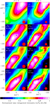 |
Fig. 1 Spatial distribution over a region of 264″×264″ of the integrated-intensity emission of the J=1–0 and J=2–1 transitions (left and right panels, respectively) of CS, C34S, 13CS, and HCS+ (from top to bottom). For each map, the integrated-line emission has been normalized to its maximum value (M). The value of M in mK km s−1 is indicated below the name of the molecule at the top left side of each panel. The HPBW of the telescope for each transition is indicated by the red circle. The central position of the map, corresponding to TMC-1(CP), is indicated by a black dot. |
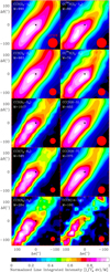 |
Fig. 2 Same as Fig. 1, but for the integrated-intensity emission, normalized to M, of several transitions of CCS (left panels), CC34S (two upper right panels) and CCCS (remaining right panels). The value of the maximum integrated intensity (in mK km s−1) is shown at the top left side of each panel. The HPBW of the telescope for each transition is indicated by the red circle. The central position of the map, corresponding to TMC-1(CP), is indicated by a black dot. |
3 Methods
The lines were identified using the MADEX catalogue (Cernicharo 2012), which contains the spectral information of 6632 species corresponding to 1853 different molecules, including their isotopologues and some of their vibrationally excited states. For some species, the CDMS (Müller et al. 2005) and the JPL (Pickett et al. 1998) catalogues were also used. The details of the spectroscopic references are given for each molecule in the next sections.
The observed line parameters were obtained by means of a Gaussian fit using the CLASS package of GILDAS4. The derived line-integrated intensities, their velocities, the antenna temperatures, and the full width at half intensity are given in Table B.1. We considered a window of ±15 km s−1 around the vLS R (5.83 km s−1) of the source for each transition to perform the fit after we removed the baseline.
The emission of all observed transitions was modelled using the large velocity gradient (LVG) approach. The basic formula and methods were described by Goldreich & Kwan (1974). This approach has been implemented in the MADEX code. In all cases, we assumed a kinetic temperature of 9 K (Tercero et al. 2024) and a representative line width of 0.6 km s−1 (see Table B.1). The densities and column densities we obtained for each species are listed in Table 1 (see details in the next sections).
For the source, we adopted a uniform brightness temperature over a disc with a diameter of 80″ (Fossé et al. 2001; Cernicharo et al. 2023). This is a reasonable approximation to the spatial extent and structure of the source. The spatial structure of the source corresponds to a filament that is tilted south-east towards north-west, however, with an angle of ~60°. The SANCHO maps (Cernicharo et al. 2023) were used to estimate the effect of the spatial structure of the source and the opacity effect for the different observed lines. Figure 1 shows the observed maps of the J=1–0 and 2–1 transitions of CS, 13CS, C34S, and HCS+.
To determine the molecular abundances in TMC-1, we adopted a total gas column density of 1022 cm−2 (Av=10 mag, Cernicharo et al. 1987), which was derived from star counts as an average value over a beam of 2′×2′. Values of the column density of H2 derived from Herschel observations of the dust emission with better angular resolution were obtained by Kirk et al. (2013) and Fehèr et al. (2016). The spatial distribution of N(H2) around TMC-1 derived with Herschel have values for AV that range from 5 mag at the border of the cloud to 25 mag at the CP position (see Fig. 1 of Navarro-Almaida et al. 2020; Fuente et al. 2019). From these maps, the value derived by Cernicharo et al. (1987) appears to be a good compromise for the angular resolution of the observations we present here, which ranges from 25″ to 56″ at the highest and lowest frequencies, respectively.
We also used the observed line-integrated intensities (W) of the same transition of two isotopologues, A and B, to derive the A/B abundance ratio. This method takes advantage of the fact that all data in the QUIJOTE line survey have a homogeneous calibration and the same pointing uncertainty. For the 3 mm line survey taken with the IRAM 30 m radio telescope, the data were gathered for a significant number of runs with different frequency coverage. Consequently, different transitions observed at different epochs can have different pointing and calibration errors. We therefore limited this method to the lines that were observed with QUIJOTE. The results could be independent of the source structure if both isotopologues were assumed to have the same excitation conditions, the same spatial structure, and optically thin emission in the considered lines. If these conditions are fulfilled, then the line integrated-intensity ratio WA/WB is proportional to N(A)/N(B) and to a function that depends smoothly on the excitation temperature, the energies of the levels involved in the transition, and the rotational constants of the two isotopologues (see Appendix A of Cernicharo et al. 2021b). Optically thin emission is expected for the double isotopologues of CS and for all the singly substituted isotopologues of the other species we studied.
Density and column densities derived from the models.
4 Results
4.1 CS
Carbon monosulfide (CS) is an important molecule in studies of the interstellar medium (ISM). It was the first confirmed sulphur-bearing species in the ISM and is commonly used as a tracer of the volume density in dense molecular clouds. It is also one of the most abundant molecules found in cold dark clouds such as TMC-1, which has permitted us to detect the lines of its five most abundant isotopologues with an unprecedented S/N. The electronic ground state of CS is 1Σ, and its dipole moment is μ = 1.958 ± 0.005D (Winnewisser & Cook 1968). A large set of laboratory rotational data was obtained for this molecule and its isotopologues in different vibrational states (Bogey et al. 1981, 1982; Ahrens & Winnewisser 1999; Kim & Yamamoto 2003; Gottlieb et al. 2003). Infrared data are also available, and they help us to constrain the high-order distortion constants of the molecule (Todd 1977; Todd & Olson 1979; Winkel et al. 1984; Burkholder et al. 1987; Ram et al. 1995; Uehara et al. 2015). We used the measured frequencies in these references to obtain Dunham mass-independent parameters and implemented them in the MADEX code. For the two transitions we considered, the difference between our frequencies and those in the CDMS (Müller et al. 2005) are below 1 kHz.
The observed intensities of the J=1–0 and J=2–1 transitions of CS and its isotopologues range from about 1.4 K for CS to ~1 mK for 13C33S (see Fig. 3 and Table B.1), that is, a dynamical range of 1400. We used the collision rate calculated by Denis-Alpizar et al. (2018) for the CS/p-H2 system to model the line profiles.
The CS abundance is probably highly underestimated because the J = 1–0 and 2–1 lines are expected to be opaque, and it cannot be used to derive isotopic abundances. These line trapping problems are clearly seen in the maps of the integrated intensity of CS and its 13CS and C34S isotopologues (see Fig. 1). The integrated intensity of the two lines of CS clearly peaks towards the NW of the maps and is shifted along the main axis of TMC-1 by more than 2′ with respect the emission of the isotopologues. Moreover, the emission of CS seems to decline towards the zone in which the isotopologues are most intense. This effect appears in the two transitions we studied. They were observed with different telescopes, the Yebes 40 m telescope for J=1–0, and the IRAM 30 m telescope for J=2–1. The result is therefore not an artefact of the observations.
The situation for CS is similar to that analysed by Cernicharo et al. (1987) for HCO+ and H13CO+. For these two species, it was found that the line profiles and the intensities reflected a huge opacity in the J=1–0 line of HCO+. A simple two-layer model was sufficient to explain the observations qualitatively. A high-density core that in the maps of Fig. 1 corresponds to the narrow filament oriented SE-NW, causes the emission of H13CO+. A surrounding envelope with a moderate density (a few 103 cm−3) still has enough molecules of HCO+ (here CS) to absorb the photons from the core and to re-emit them over a large volume. The line opacity in the envelope is so high that photons from the core do not escape from the cloud. The column density of the cloud is not sufficent for H13CO+ (here, 13CS and C34S) to produce significant intrinsic emission or notable absorption of the photons from the dense filament, however. This situation is typical of cold clouds with narrow line widths and small velocity gradients. As a consequence, all points of the cloud with a high and low volume density are connected radiatively.
The two-layer model is an oversimplification of the radiative transfer problem in TMC-1, and a more detailed analysis is required to implement density and velocity gradients from the external parts to the core. To achieve these goals, we require a multi-line study with a higher angular resolution than we used here. Nevertheless, we tested the reliability of the model by comparing the predicted intensities for all the isotopologues of CS with the observations.
A direct determination of the 12C/13C abundance ratio in CS can be derived from the line intensities of C34S and 13C34S. We estimated, however, that the J=1–0 and J=2–1 lines of C34S have opacities of ~0.5 and 1.6, respectively. The ratios we obtained from the direct comparison of the line intensities are therefore to be considered lower limits. From the J=1–0 line intensities, we obtained 12C/13C=54.9±0.7. From the J=2–1 transition, we derived a ratio of 44.0±6.5. Nevertheless, the column densities for C34S and 13C34S were determined from the LVG approximation used for CS, and these opacity corrections are therefore taken into account in our estimation of the column densities in Table 1. From the LVG calculations, we derived a 12C/13C abundance ratio of 90±9.
Two of the three hyperfine components of the J=1–0 transition of 13C33S are marginally detected in the QUIJOTE line survey. In the next months, improved QUIJOTE data might allow us to improve the data for this rare isotopologue of CS and to derive a better isotopic 12C/13C abundance ratio from C33S and 13C33S.
The derived column densities for the different isotopologues of CS are given in Table 1. The derived isotopic abundances from these column densities are given in Table 2 and are discussed in Section 4.6.
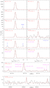 |
Fig. 3 Observed J = 1–0 and 2–1 lines of CS and its isotopologues 13CS, C34S, C33S, and 13C34S toward TMC-1. For C36S and 13C33S, only the J=1–0 line was detected. The abscissa corresponds to the local standard of rest velocity of the lines adopting the rest frequencies given in Table B.1. In the two bottom panel, however, the abscissa corresponds to the rest frequency. The ordinate corresponds to the antenna temperature corrected for atmospheric and telescope losses in mK. The derived line parameters for the observed lines are given in Table B.1. The synthetic spectra (red line) are derived for the column densities shown in Table 1 and the LVG model described in Sections 3 and 4.1. For CS, a two-layer component model is used (see Section 4.1). Negative features appearing in the folding of the frequency switching data are blanked in all the figures. The observed spectrum of the hyperfine component J=1–0, F=1/2–3/2 of C33S was multiplied by 0.1. |
4.2 HCS+
This molecule was found in space in 1981 by Thaddeus et al. (1981) prior to any laboratory measurement through the observation of four lines that were related harmonically. The identification was confirmed by the observation of the J=2–1 line in the laboratory by Gudeman et al. (1981). Precise rotational constants for HCS+ and several of its isotopologues were derived from laboratory measurements by different authors (Bogey et al. 1984; Tang & Saito 1995; Margulès et al. 2003). It is interesting to note that the dipole moment of this species is 1.958 D (Botschwina & Sebald 1985), which is identical to that of CS. Therefore, we assumed as a first approximation that CS and HCS+ undergo the same excitation conditions, which depend on the Einstein coefficients and collisional rate coefficients, and derived their abundance ratios using the intensity ratios of optically thin lines. HCS+ is chemically related to CS as it results from the protonation of this species with H3+, HCO+, and H3O+ as the main proton donators. Its principal destruction path is through electronic dissociative recombination to produce CS.
We report the detection of the J=1–0 and 2–1 lines of HCS+, H13CS+, HC34S+ and, for the first time in space, of HC33S+. The rotational constants for this isotopologue were derived from the observed line frequencies, as discussed in Appendix A.6. Figure 4 shows the observed lines of all isotopologues of HCS+. The spatial distribution of the J=1–0 and J=2–1 lines of HCS+ is shown in Fig. 1. The emission from the two transitions appears to be very similar to that of C34S and 13CS, which indicates that CS and HCS+ coexist spatially. Like for CS, the emission peak is shifted relative to our central position. The change in intensity between the emission peak and the central position is smaller than 15%.
Using the same parameters for the source as for CS and the collisional rate coefficients calculated by Denis-Alpizar et al. (2022) for HCS+ with p-H2, we derived a volume density from the observed lines of n(H2)=1.0×104 cm−2. For the main isotopologue the best fit to the line profiles was obtained for a slightly lower value of the volume density (0.9×104 cm−3). This fact, together with the observed line intensity ratios between HCS+ and its rare isotopologues, suggests minor opacity problems for its lines. The computed LVG opacity values for HCS+ are τ(J=1–0)~0.19 and τ(J=2–1)~0.76. The best fits to the column densities are given in Table 1, and the comparison between the modelled and observed spectra is shown in Fig. 4. The opacity of the lines of all isotopologues is much lower and does not affect our column density estimates. For HCS+, the column densities derived from the LVG analysis take the line opacities into account as a first approximation.
The isotopic abundance ratios derived from HCS+ and its isotopologues are given in Table 2. The HCS+/H13CS+ column density ratio is 91±9. Using the integrated line intensities of the J=1–0 of HCS+ and H13CS+, we obtained 12C/13C=78±3, and from the J=2–1 transition line, we derived an abundance ratio of 82 ± 2. Both determinations are nearly identical to the determination derived from C34S and 13C34S. This value also agrees with the 12C/13C averaged abundance ratio derived from the 13C isotopologues of C4H (Sakai et al. 2013), of HC5N (Takano et al. 1998; Cernicharo et al. 2020) and of HCCCN, HNCCC, and HCCNC (Cernicharo et al. 2024a; Tercero et al. 2024).
The abundance ratios of the protonated and neutral molecule depend on the degree of ionisation and on the formation and destruction rates of the cation. These ratios also increase with the proton affinity of the neutral species (Agúndez et al. 2015). From the derived column densities for the isotopologues of CS and HCS+, we derived N(13CS)/N(H13CS+) = 43 ±4, N(C34S)/N(HC34S+) = 40 ±4 and N(C33S)/N(HC33S+) = 34 ±4. Based on this, the abundance ratio of CS and its protonated form in TMC-1 is ~40.
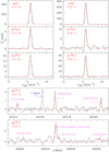 |
Fig. 4 Observed J = 1–0 and 2–1 lines of HCS+ and its isotopologues towards TMC-1. The abscissa corresponds to the local standard of rest velocity of the lines adopting the rest frequencies given in Table B.1. The bottom panels show the same transitions of HC33S+, which exhibit several hyperfine components. The abscissa in this case is the rest frequency adopting a velocity for the source of 5.83 km s−1 (Cernicharo et al. 2020). The ordinate corresponds to the antenna temperature corrected for atmospheric and telescope losses in mK. The derived line parameters for the observed lines are given in Table B.1. The synthetic spectra (red line) are derived for the column densities shown in Table 1 and the LVG model described in Sections 3 and 4.2. |
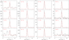 |
Fig. 5 Observed lines of CCS towards TMC-1. The abscissa corresponds to the local standard of rest velocity of the lines adopting the rest frequencies given in Table B.1. The ordinate corresponds to the antenna temperature corrected for atmospheric and telescope losses in mK. The derived line parameters are given in Table B.1. The synthetic spectra (red line) are derived for the column densities shown in Table 1 and the LVG model described in Section 3 with n(H2)=1.3×104 cm−3 and N(CCS)=3.4×1013 cm−2 (see Section 4.3). |
4.3 C2S
The linear molecule CCS (thioxoethenylidene) has a 3Σ− ground electronic state. It was first identified in the ISM towards TMC-1 and Sgr B2 (Saito et al. 1987; Yamamoto et al. 1987; Kaifu et al. 1987) and towards the carbon-rich evolved star IRC+10216 (Cernicharo et al. 1987). Nevertheless, one of its rotational lines was previously reported by Suzuki et al. (1984) towards TMC-1, but lack of laboratory spectroscopy at that time prevented the assignment of the line to CCS. All the laboratory-measured frequencies of CCS (Saito et al. 1987; Yamamoto et al. 1990; Lovas et al. 1992; McGuire et al. 2018) were used to fit a standard Hamiltonian for a 3Σ molecule. The resulting rotational constants were implemented in the code MADEX. The predicted frequencies for the transitions we observed are given in Table B.1. The dipole moment of CCS was calculated to be 2.88 D (Pascoli & Lavendy 1998; Lee 1997). In the Q band, we detected four lines for the CCS molecule and its most abundant isotopologue CC34S (see Figures 5 and 6, and Table B.1), which correspond to the transitions with N=2 up to 4 (J=N±0,1). The intensities of two of these transitions lie above 100 mK.
On the other hand, for the 13CCS, C13CS, and C13C34S isotopologues, we observed the transitions NJ = 23–12 and NJ = 34–23 (see Fig. 7), and all their hyperfine components were detected with a good S/N.
We obtained the line parameters for thioxoethenylidene (CCS) using the same methods as for the previous molecules, and we report them in Table B.1. We also calculated the column densities using the set of collisional rate coefficients computed by Godard Palluet & Lique (2023, 2024) and the LVG approach. These values are given in Table 1.
Several unidentified lines were detected in our survey in the Q band with different patterns at 33.4 GHz and 44.9 GHz. Based on the CCS data and the expected abundances for the 33S isotopologue, we suspect that these lines correspond to the hyperfine structure of the CC33S molecule. To confirm this assignment, we used ab initio theoretical calculations and laboratory data (see Appendix A.2). These transitions correspond to NJ = 23–12 and NJ = 34–23 (see Fig. 8). We obtained the observed line parameters and report them in Table B.1.
The spatial distribution of CCS and its isotopologue CC34S follows the same behaviour as observed for CS and its isotopologues (see Fig. 2). For the J = 89–78 transition, however, the distribution is split into two peaks that follow the same SE-NW orientation.
Because the lines are opaque, we performed several calculations to obtain the most accurate column density for the molecules that lack a hyperfine structure (CCS and CC34S) by varying the density between 102 and 108 cm−3 for three values of the column densities (1012, 1013 and 1014 cm−2). These values represent abundances with respect to H2 from 10−10 to 10−12. For both molecules, we found that the most intense transitions are 23–12 and 34 − 23, with the latter being the largest of them. These transitions thermalise at lower values than the other two transitions. For these values, we found that the best-fit column density corresponds to 2.8 × 1013 cm−2 in the case of CCS and 1.0 × 1012 cm−2 for the CC34S isotopologue. These two results correspond to a density of 1.3 ×104 cm−3.
Isotopic ratio derived from S-bearing molecules in TMC-1.
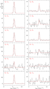 |
Fig. 6 Observed lines of CC34S towards TMC-1. The abscissa corresponds to the local standard of rest velocity of the lines adopting the rest frequencies given in Table B.1. The ordinate corresponds to the antenna temperature corrected for atmospheric and telescope losses in mK. The derived line parameters are given in Table B.1. The synthetic spectra (red line) are derived from the LVG model described in Section 3 with n(H2)=1.3×104 cm−3 and N(CC34S)=1.5×1012 cm−2 (see Section 4.3). |
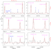 |
Fig. 7 Observed hyperfine components of the NJ = 23−12 (left panels) and NJ = 34–23 (right panels) transitions of 13CCS, C13CS, and C13C34S towards TMC-1. The abscissa corresponds to the rest frequency in MHz. The ordinate corresponds to the antenna temperature corrected for atmospheric and telescope losses in mK. The derived line parameters are given in Table B.1. The synthetic spectra (red line) are derived from the LVG model described in Section 3 with n(H2)=1.3×104 cm−3 and the column densities given in Table 1 (see Section 4.3). |
4.4 CCCS
The linear molecule CCCS has an electronic ground state 1Σ. Abundant laboratory data of its rotational transitions and those of its isotopologues were reported (Yamamoto et al. 1987; Lovas et al. 1992; Tang & Saito 1995; Ohshima & Endo 1992; Gordon et al. 2001; Sakai et al. 2013; McGuire et al. 2018). Its dipole moment was measured to be μ = 3.704D (Suenram et al. 1994). The first detection of CCCS in space was achieved towards TMC-1 (Kaifu et al. 1987; Yamamoto et al. 1987) and towards the carbon-rich evolved star IRC+10216 (Cernicharo et al. 1987). We fitted the available laboratory data for each isotopologue of CCCS and implemented them into the MADEX code. The frequencies we used for the observations are given in Table B.1.
In our observations, we detected three transitions of CCCS, CCC34S, 13CCCS, and C13CCS in the Q band corresponding to J = 8–7, J = 7–6 and J = 6–5. In addition, CCCS lines from J = 13–12 up to J = 18–17 were detected with the IRAM 30 m telescope line survey in the 3 mm domain. The lines of CCCS and its isotopologues are shown in Figs. 9 and 10. The derived line parameters of the observed lines were obtained using the same methods as for the previous molecules and are given in Table B.1. Because the rotational constants of CCCS and those of CC13CS are nearly coincident, the latter isotopologue could not be detected (its transitions differ by less than 0.1 MHz from those of CCCS and are not resolved in the QUIJOTE data). We detected several features at 34.2, 39.6, and 45.6 GHz that correspond to the isotopologue CCC33S. Improved rotational constants from our measured line frequencies in TMC-1 and those obtained from previous (McGuire et al. 2018) and new laboratory data are given in Appendix A.4 and Table A.6.
The spatial distribution of CCCS is very similar to that of the isotopologues of CS, HCS+, CCS, and CC34S as shown in Fig. 2, which can be compared to the maps in Fig. 1. The emission peak of CCCS, like the other species in Figs. 1 and 2, is shifted to Δα = −30″ and Δδ = −30″ with respect to the centre of the maps, but the intensity variation between this position and the central one is smaller than 15%. For J = 14–13, similar to the CCS case, the distribution is split into two peaks, with a higher intensity located to the SE. Again, the assumption of a source of uniform brightness over a diameter of 80″ seems to be a reasonable hypothesis.
Collisional rate coefficients for CCCS with He were calculated by Sahnoun et al. (2020). Only 11 levels were considered (Jmax=10), however, that only cover energies up to 15.3 K. These rates cannot be used to model the nine observed lines of CCCS, which go from J=6–5 up to J=18–17, with upper-level energies up to 47.5 K, which is well above the energies calculated by Sahnoun et al. (2020). The detection of these high-J lines of CCCS provides a key constraint in the modelling of the observed intensities. An estimation of the collisional rate coefficients above Ju=10 can be obtained from the σ(0→J) cross sections with the IOS approximation. This approach, however, introduces several uncertainties in the modelling of the high-J lines. The available collisional rate coefficients between CCCS and He are similar to those of the HCCCN with p-H2 (Faure et al. 2016). We therefore adopted the HCCCN-p-H2 rate coefficients to model the observed CCCS lines.
In order to fit the lines of CCCS, we explored the predicted intensities and line intensity ratios for a wide range of volume densities. Surprisingly, the best fit to the data was obtained for n(H2)=(1.3±0.2)×104, which is the same value as for CCS. Figure 9 shows the quality of the synthetic line profiles obtained from our model for N(CCCS)=(6.8±0.7)×1012 cm−2. The largest discrepancy is observed for the J = 15–14 line. It is due to the severe blending of this transition with a feature arising from HCO, however. The lines of the four isotopologues of CCCS, 13CCCS, C13CCS, CCC34S, and CCC33S are reproduced very well with the same model and for the column densities given in Table 1.
The column density ratio of CCCS and 13CCCS is 309±30, while for CCCS/C13CCS, the value is 92±9, which is nearly identical to the solar abundance 12C/13C. These species were previously studied in TMC-1 by Sakai et al. (2013), who derived values for these ratios of ≥209 and 48±15. Our more sensitive observations (at least a factor of 10) clearly indicate that C13CCS has an isotopic abundance ratio slightly higher than that of the local ISM standard value of 60–70. The abundance of 13CCCS is depleted by a factor 3.4±0.3. The abundance ratio of CCCS and CCC34S is 25.2±2.5, which is identical to the solar abundance. The derived isotopic ratios are given in Table 2 and are discussed in Section 4.6.
4.5 H2CS and other S-bearing species
TMC-1 is known to be a factory of sulphur-bearing species (Cernicharo et al. 2021c). In addition to the species considered in previous sections, other molecules such as NCS, HCCS, H2CS, H2CCS, H2CCCS, HCCCCS, HCSCN, HCSCCH, HCCS+, HCCCS+, C4S, and C5S were recently detected with the QUIJOTE line survey (Cernicharo et al. 2021b,c,d; Cabezas et al. 2022a; Fuentetaja et al. 2022). When the observed line intensities of these species and their associated column densities are taken into account (see Table 1 of Cernicharo et al. 2021c), the abundances of H2CS (Cernicharo et al. 2021c), HCCS+ (Cabezas et al. 2022a), and HCSCN (Cernicharo et al. 2021d) alone are high enough to allow the detection of their 34S and 13C isotopologues in our line survey.
For H2CS our data from QUIJOTE and the IRAM 30 m telescope observations cover two ortho and two para transitions. They are detected for H2CS, H2C34S, and H213CS, and the observed lines are shown in Fig. 11. In addition, the three hyperfine components of the 101–000 transition of H2C33S were also detected in space for the first time. They are shown in Fig. 11, and the derived line parameters are given in Table B.1. In spite of the high observed intensities for the lines of H2CS, the emission seems to be optically thin because the intensity ratios of H2CS and its isotopologues for the four observed lines are near the solar abundance of 12C/13C and 32S/34S.
No collisional rate coefficients are available for H2CS, but they can be inferred from those of H2CO. Two different sets of collisional rate coefficients can be employed for o-H2CS, those of collisions of H2CO with He (Green 1991), or those of collisions with o-H2 and p-H2 calculated by Troscompt et al. (2009). For p-H2CS, only the p-H2CO-He rate coefficients (Green 1991) can be employed. The results of our LVG models using the rate coefficients of o/p-H2CS with He are shown in Fig. 11. It is surprising to find that the fitted line profiles reproduce the two para and one of the ortho lines of the three isotopologues quite well. The volume density adopted in the model is 1.5×104 cm−3, but when the large uncertainty on the adopted rate coefficients is taken into account, this density has to be taken with caution. In the modelling, we found an ortho-to-para ratio for all isotopologues of 2.0±0.1, which is significantly different from the expected value of 3. The main discrepancy between observations and the model was found for the ortho 313 − 212 transition, for which the predicted intensities have to be multiplied by a factor ~0.5 to match the observations (see Fig. 11; the correction factor for the 313 − 212 transition is specified for each isotopologue). The computed excitation temperature for this transition is very sensitive to the adopted volume density. The computed line opacities for the two observed ortho transitions are identical, however. Hence, the brightness temperature is always higher for the 313–212 transition than for the 312 − 211 one. We explored the effect of the volume density on the expected intensities. For higher values of n(H2), all lines are too strong. We also analysed the effect of the adopted collisional rate coefficients. Using the rate coefficients of o-H2CO with p-H2 of Troscompt et al. (2009), we obtained an intensity ratio for the two ortho lines, TB(313 − 212)/TB(312 − 211), of 1.34; but for the collisional rate coefficients with He (Green 1991), this ratio is 1.94. Consequently, the observed intensity discrepancy between the two ortho line seems to be related to the set of collisional rate coefficients adopted for H2CS. Unfortunately, the data of Troscompt et al. (2009) only cover ten energy levels of o-H2CO (for H2CS, this corresponds to a maximum enery of 22 K) and were not calculated for p-H2CO. In the final model, we therefore adopted the collisional data of H2CO with He and applied the correction factor to the intensity of the 313 − 212 transition. The derived ortho/para ratio has to be taken with caution. Future calculations for the collisional rate coefficients of thioformaldehyde with He and/or H2 will be very interesting. This molecule is ubiquitous in space, and its lines are easily detected in cold, warm, and hot molecular clouds. It is also detected in evolved stars (Agúndez et al. 2008).
The column density ratios given in Table 2 indicate that 12C/13C and 32S/34S are similar to the solar abundances. These abundance ratios can be also obtained from the line intensity ratios between the different isotopologues (see Table B.1 and Fig. 11). From the four lines of each of them, we derived an averaged value for 12C/13C and 32S/34S of 84.7±3 and 24.9±1, respectively. These isotopic abundance ratios are similar to those derived from S-bearing species that only contain one carbon (CS and HCS+).
HCCS+ has been detected in TMC-1 by Cabezas et al. (2022a). The identification was based on ab initio calculations and the detection of 26 of its rotational transitions, which contain fine and hyperfine structure. The intensity of the lines of HCCS+ is high enough to allow the detection at least of the 34S isotopologue. Based on the rotational constants predicted for HCC34S+, from our ab initio calculations and those observed for HCCS+, we predict the frequencies of the four strongest lines of HCC34S+ in the QUIJOTE domain (see Section A.5). Four lines are found at frequencies that differ from the predicted values by less than 0.1 MHz. They are shown in Fig. 12, and their line parameters are given in Table B.1. A fit to the observed frequencies provides accurate rotational constants of this species (see Section A.5). To derive a column density for this isotopologue, we adopted the rotational excitation temperature derived for CC34S for all hyperfine components of each rotational transition of HCC34S+ and derived a column density of 4.7×1010 cm−2. From the column density of HCCS+ derived by Cabezas et al. (2022a), we derived a 32S/34S abundance ratio of 23.4±2.5, which is similar to that obtained from other species. The expected intensities for the 13C isotopologues, ~0.15–0.3 mK, are below the current sensitivity of QUIJOTE.
The abundance ratios of the protonated and the neutral molecule are similar to those of the HCS+/CS cases. We obtained a value of 30.9 for N(HCCS+)/N(CCS) and 31.9 for the N(HCC34S+)/N(CC34S) ratio.
The rotational constants for HC34SCN were obtained by Cernicharo et al. (2021d). From the intensities observed for the main isotopologue (Cernicharo et al. 2021d), the expected intensities for the strongest transitions of HC34SCN are ~0.4 mK. An exploration of the QUIJOTE data provides the detection of only three lines at 3σ, while other lines remain undetected. Future improved QUIJOTE data might allow us to detect this isotopologue of HCSCN.
We also considered C4S and C5S. They are analysed in Appendices A.7 and A.8, respectively. Their observed intensities are too low, ~1 mK, to permit the detection of their isotopologues. Nevertheless, improved rotational constants for both molecules are provided in Tables A.10 and A.11, respectively.
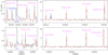 |
Fig. 8 Observed hyperfine components of the NJ = 23−12 (upper panels) and NJ = 34–23 (bottom panels) transitions of CC33S towards TMC-1. The derived line parameters of the observed lines are given in Table B.1. The abscissa corresponds to the rest frequency in MHz. The ordinate corresponds to the antenna temperature corrected for atmospheric and telescope losses in mK. The synthetic spectra (red line) are derived from the LVG model described in Section 3 with n(H2)=1.3×104 cm−3 and N(CC33S)=3.5×1011 cm−2 (see Section 4.3). |
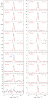 |
Fig. 9 Observed transitions of CCCS, CCC34S, 13CCCS, and C13CCS towards TMC-1. All transitions of CCCS are shown in the left panels. The right panels show J=6–5, 7–6, and 8–7 of the three isotopologues. The abscissa corresponds to the local standard of rest velocity of the lines adopting the rest frequencies given in Table B.1. The ordinate corresponds to the antenna temperature corrected for atmospheric and telescope losses in mK. The derived line parameters are given in Table B.1. The synthetic spectra (red lines) have been calculated from the LVG model described in Section 4.4. The adopted volume density is n(H2)=1.3×104 cm−3 for all isotopologues, and the resulting column densities are given in Table 1. |
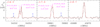 |
Fig. 10 Observed transitions of CCC33S towards TMC-1. The abscissa corresponds to the rest frequency. The ordinate corresponds to the antenna temperature corrected for atmospheric and telescope losses in mK. The derived line parameters are given in Table B.1. The synthetic spectra (red line) are derived from a model with N=6.2x1010 cm−2 and Trot=8 K (see Section 4.4). |
4.6 Discussion
From the column densities, we calculated for the various species as summarized in Table 1, we derived the corresponding abundance ratios, which are given in Table 2, where they are compared with the values derived in the dark cloud L483 and in the Solar System. The abundance ratios CS/C34S and CS/13CS are not reliable because the J = 1–0 and J = 1–0 lines of CS are affected by opacity. This limitation can be overcome using the doubly substituted isotopologue 13C34, which yields 32S/34S and 12C/13C ratios that agree with those derived using H2CS and HCS+. The 32S/34S ratios derived in TMC-1, in the range 22.0–25.2, are consistent with the Solar System value of 22.6 and with the values derived in the local ISM, 24.4±5.0 (Chin et al. 1996), 19±8 (Lucas & Liszt 1998), and ~22 (Wilson 1999). The values found in L483 are also consistent within the errors with the local ISM and Solar System values. On the other hand, the 13C33S ratios in TMC-1, in the range 68.8–109.7, are somewhat lower than the Solar System value of 127 and the local ISM value of 153±40 (Chin et al. 1996). It therefore seems that there is minimal isotopic fractionation for 34S, while there could be a slight isotopic enrichment in 33S in TMC-1. In the case of carbon, the 12C/13C ratios derived from C34S, C33S, H2CS, and HCS*, which are in the range 82.2–91, are consistent with the Solar System value of 89 and somewhat above the local ISM values of 59±2 (Lucas & Liszt 1998), 69±6 (Wilson 1999), 68±15 (Milam et al. 2005), 70±2 (Sheffer et al. 2007), 76±2 (Stahl et al. 2008), and 74.4±7.6 (Ritchey et al. 2011). The fact that the values found in the local ISM are systematically lower than those found in TMC-1 suggests that they might be affected by opacity, resulting in an underestimation of the true 12C/13C interstellar ratio. The 12C/13C ratios derived from CCS and CCCS deserve special attention. Isotopic ratios are very different and depend on the position where 13C is substituted. In general, the isotopologue with a 13C at the terminal carbon exhibits a much lower abundance than the other observed isotopologue. These isotopic anomalies were first noted by Sakai et al. (2007) for the CCS isotopologues and later on by Sakai et al. (2013) for CCCS. The explanation of these isotopic anomalies have been the subject of discussion. It was originally proposed that the formation pathway of the molecules themselves with non-equivalent carbon atoms was at the origin Sakai et al. (2007). A different explanation was proposed by Furuya et al. (2011), who suggested that the different abundances of the various isotopologues might be caused by isotopologue exchange reactions involving H atoms. These reactions would progressively transform the less stable isotopologues into the more stable one approaching abundance ratios determined by the difference in the zero-point energies (ZPE) of the different isotopologues. The scenario proposed by Furuya et al. (2011) was validated by Talbi (2018), who studied the exchange reaction 13CCS + H → C13CS + H theoretically and found it to be barrierless. If this reaction is rapid enough, it would indeed tend to drive the C13CS/13CCS abundance ratio to a value of exp(ΔE/T), where T is the gas kinetic temperature, and ΔE is the difference between the ZPE of 13CCS and that of C13CS. For a value of ΔE of 18.9 K (Talbi 2018), the theoretically expected C13CS/13CCS would be 8.2 for a kinetic gas temperature of 9 K (Agúndez et al. 2023), which is only slightly above the observed value in TMC-1 of 6.8. Isotopic fractionation of carbon was studied using chemical models (Roueff et al. 2015; Colzi et al. 2020; Loison et al. 2020). The implementation of the H exchange mechanism in the chemical model of Loison et al. (2020) resulted in a C13CS/13CCS ratio that was somewhat lower than observed, in the range 1–4, depending on the time and on the assumptions about the O + C3 reaction. It would be interesting to further explore which conditions allow us to reproduce the observed C13CS/13CCS ratio and also to explore the isotopic anomalies found for CCCS.
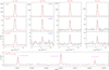 |
Fig. 11 Observed transitions of H2CS and its isotopologues towards TMC-1. The abscissa corresponds to the local standard of rest velocity of the lines adopting the rest frequencies given in Table B.1, except for the bottom panel (H2C33S) for which it corresponds to the rest frequency. The ordinate corresponds to the antenna temperature corrected for atmospheric and telescope losses in mK. The derived line parameters are given in Table B.1. The synthetic spectra (red line) are derived from the LVG model described in Section 4.5. The modelled spectra for the 313−212 transition of H2CS, H2C34S and H213CS have been multiplied by a correction factor indicated in blue at the top right side of the corresponding panels. For all the other transitions, no correction factors are applied. This factor results from the adopted collisional rate coefficients for H2CS (see Section 4.5). |
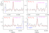 |
Fig. 12 Observed lines of HCC34S+ towards TMC-1. The abscissa corresponds to the rest frequency. The ordinate corresponds to the antenna temperature corrected for atmospheric and telescope losses in mK. The derived line parameters of the observed lines are given in Table B.1. The modelled spectra (red line) are derived for N(HCC34S+)=4.7×1010 cm−2 adopting the kinetic temperatures calculated for CC34S as the rotational temperature for n(H2)=1.3×104 cm−3. |
5 Conclusions
We have presented a comprehensive analysis of the CS, CCS, CCCS, C4S, C5S, and H2CS molecules and their isotopologues detected towards TMC-1 using the QUIJOTE line survey conducted with the Yebes 40 m radio telescope. A total of 69 lines were observed, including the first detection of C36S in this source. For the line-fitting procedure, we employed specific collisional rate coefficients and analysed the line intensity ratios for four of the studied species. We also presented a laboratory study of rotational spectroscopy for the CC33S and CCC33S species, theoretical calculations for HCC34S+, and improved values of the rotational constants of other species detected based on the observations.
Our analysis of the abundance ratios derived from different isotopologues provides the most complete information to date on isotopic ratios for these molecules in TMC-1. These ratios were compared in detail with Solar System values, and we revealed a consistency and offered insights into isotopic fractionation processes within the cloud. Additionally, we analysed the abundance ratios of the protonated and neutral species, specifically, for CS and CCS, through their respective isotopologues. We also commented on the anomaly observed in the 13C isotopologues of CCS and CCCS and analysed its possible causes. Furthermore, we investigated the spatial distribution of the most abundant molecules within TMC-1, where we observed a distribution pattern that is consistent with the expected pattern. This spatial analysis enhances our understanding of the molecular environment and the chemical processes governing the molecule formation and distribution in dark cold clouds.
Data availability
Table B.1 is available at the CDS via https://cdsarc.cds.unistra.fr/viz-bin/cat/J/A+A/702/A23.
Acknowledgements
We thank Ministerio de Ciencia e Innovación of Spain (MICIU) for funding support through projects PID2019-106110GB-I00, PID2019-107115GB-C21/AEI/10.13039/501100011033, and PID2023-147545NB-I00. We also thank ERC for funding through grant ERC-2013-Syg-610256-NANOCOSMOS. C.C., Y.E., M.A, and J.C. thank Ministry of Science and Technology of Taiwan and Consejo Superior de Investigaciones Científicas for funding support under the MOST-CSIC Mobility Action 2021 (Grants 11-2927-I-A49-502 and OSTW200006). A.G.P. and F.L. acknowledge financial support from Rennes Metropole and the European Research Council (Consolidator Grant COLLEXISM, Grant Agreement No. 811363), the CEA/GENCI (Grand Equipement National de Calcul Intensif) for awarding them access to the TGCC (Très Grand Centre de Calcul) Joliot Curie/IRENE supercomputer within the A0110413001 project and from the Institut Universitaire de France.
Appendix A Spectroscopic data
A.1 New molecular constants for 13CCS and C13CS species
The observed lines of 13CCS and C13CS species (see Table B.1) were merged with the laboratory data (Yamamoto et al. 1990; Ikeda et al. 1997) to provide a new set of molecular constants using the SPFIT code (Pickett 1991). They are given in Tables A.1 and A.2.
New spectroscopic parameters of 13CCS
New spectroscopic parameters of C13CS.
Observed laboratory transition frequencies for CC33S
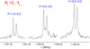 |
Fig. A.1 Laboratory measurements of the three hyperfine components of the NJ=21−10 rotational transition of CC33S we observed. The abscissa corresponds to the frequency of the lines in MHz. The spectra were achieved by 100-shots of accumulation. The coaxial arrangement of the adiabatic expansion and the resonator axis in the FTMW spectrometer produces an instrumental Doppler doubling. The resonance frequencies are calculated as the average of the two Doppler components. |
A.2 Laboratory spectroscopy data for CC33S
The rotational spectrum of the CC33S radical was observed using a Balle-Flygare narrowband type Fourier-transform microwave (FTMW) spectrometer operating in the frequency region of 4-40 GHz (Endo et al. 1994; Cabezas et al. 2016). The short-lived species CC33S was produced in a supersonic expansion by a pulsed electric discharge of a gas mixture of CS2 (0.3%) and C2H2 (0.3%) diluted in Ar. This gas mixture was flowed through a pulsed-solenoid valve that is accommodated in the backside of one of the cavity mirrors and aligned parallel to the optical axis of the resonator. A pulse voltage of 1400 V with a duration of 450 μs was applied between stainless steel electrodes attached to the exit of the pulsed discharge nozzle (PDN), resulting in an electric discharge synchronized with the gas expansion. The resulting products generated in the discharge were supersonically expanded, rapidly cooled to a rotational temperature of ~2.5 K between the two mirrors of the Fabry-Pérot resonator, and then probed by FTMW spectroscopy. For measurements of the paramagnetic lines, the Earth’s magnetic field was cancelled by using three sets of Helmholtz coils placed perpendicularly to one another. Since the PDN is arranged parallel to the cavity of the spectrometer, it is possible to suppress the Doppler broadening of the spectral lines, allowing to resolve small hyperfine splittings. The spectral resolution is 5 kHz and the frequency measurements have an estimated accuracy better than 3 kHz.
Quantum chemical calculations were carried out to estimate the molecular parameters of CC33S. Very precise values for the rotational constant can be obtained using experimental/theoretical ratios derived for CCS parent species. This is the most common method to predict the expected experimental rotational constants for an isotopic species of a given molecule when the rotational constants for its parent species are known. The calculations were done using the second order Møller-Plesset perturbation (MP2; Møller & Plesset 1934) and Dunning’s augmented correlation-consistent polarized quadruple-ζ basis sets (aug-cc-pVQZ; Dunning 1989). This calculations were carried out using the Gaussian16 (Frisch et al. 2016) program package. For the frequency predictions, other parameters determined for the parent species CCS (Yamamoto et al. 1990) were used.
Spectroscopic parameters of CC33S
We observed by FTMW spectroscopy, two rotational transitions with quantum numbers NJ=21−10 and 12−21 at 11 and 22 GHz, respectively. An example is shown in Figure A.1. Each transition is split into several hyperfine components due to the presence of the 33S nucleus, which has a non-zero nuclear spin. The frequencies for all these hyperfine components (see Table A.3) and those observed in TMC-1 were analysed with the SPFIT program (Pickett 1991) using a Hamiltonian for a linear molecule in a 3Σ electronic state. The employed Hamiltonian can be written as follows:
![Mathematical equation: $\[H=H_{r o t}+H_{s s}+H_{s r}+H_{m h f},\]$](/articles/aa/full_html/2025/10/aa54035-25/aa54035-25-eq2.png) (A.1)
(A.1)
where Hrot, Hss, and Hsr denote the rotational, spin-spin, and spin-rotation terms, respectively, and Hmhf represents the magnetic hyperfine coupling interaction term due to the 33S nucleus. The coupling scheme used is J = N + S, F = J + I(33S).
The molecular constants determined from the fit are given in Table A.4. We determined the B rotational constant, the spinspin interaction constant, λ, and the hyperfine constants for the 33S nucleus, named Fermi contact constant, bF, the dipole-dipole constant, c, and the nuclear quadrupole coupling constant, eQq. Other parameters like the distortion constant, D, and the spinrotation interaction constants, γ and γD, were kept fixed to the values determined for the parent species CCS (Yamamoto et al. 1990).
A.3 C13C34S
Using similar theoretical and experimental methods than for CC33S we explore the rotational spectrum of C13C34S. We detected four unidentified lines in our survey in the Q-band very close to the predicted frequencies at 32.9 and 42.3 GHz. They were attributed to the most intense hyperfine components of the rotational transitions with quantum numbers NJ=23−12 and 34−23, respectively. Each transition is split in two intense hyperfine components due to the presence of the 13C nucleus, which has a non-zero nuclear spin. The frequencies for these four hyperfine components were analysed with the SPFIT program (Pickett 1991) using the Hamiltonian for a linear molecule in a 3Σ electronic state described above. The molecular constants determined from the fit are given in Table A.5. We determined the B rotational constant and the spin-spin interaction constant, λ. Other parameters were kept fixed to the values determined for CCS, and CC34S (Yamamoto et al. 1990; Ikeda et al. 1997), and for C13CS determined here (see A.1).
Spectroscopic parameters of C13C34S
Spectroscopic parameters of CCC33S
A.4 CCC33S
The rotational spectrum for the CCC33S species has been observed in the laboratory by (McGuire et al. 2018), who reported the observation of nine hyperfine components. In this work, we measured the rotational transition for CCC33S in the 10-34 GHz frequency region and we observed a total of 23 hyperfine components. The measured frequencies are given in Table A.7. The experimental setup and experimental conditions are the same that those used in this work for CC33S.
Towards TMC-1 we observe two well resolved hyperfine components for the J=6-5 transition. The J=7-6 transition appears as two overlapping lines, while for the transition J=8-7 the hyperfine structure is collapsed into a single feature (see Figure 10). All the observed laboratory frequencies, together with those observed in TMC-1 (see Table B.1), were analysed using the SPFIT program (Pickett 1991), using a Hamiltonian for singlet linear molecules, with the following form: H = Hrot + Hnqc where Hrot contains rotational and centrifugal distortion parameters and Hnqc the nuclear quadrupole coupling interactions. The coupling scheme used is F = J + I(33S). The analysis rendered the experimental constants listed in Table A.6.
A.5 HCC34S+
The HCC34S+ isotopic species has not been observed before in the laboratory nor in space. The rotational constant for this isotopologue can be estimated from quantum chemical calculations as shown above for other species as CC33S. We detected four unidentified lines in our survey in the Q-band very close to the predicted frequencies at 31.4 and 42.1 GHz (see Fig. 12 and Table B.1). They were attributed to the most intense hyperfine components of the rotational transitions with quantum numbers NJ=23−12 and 34−23, respectively. Each transition is split in two intense hyperfine components due to the presence of the hydrogen nucleus, which has a non-zero nuclear spin. The frequencies for these four hyperfine components were analysed with the SPFIT program (Pickett 1991) using a Hamiltonian for a linear molecule in a 3Σ electronic state. The employed Hamiltonian has been described above. The analysis rendered the experimental constants listed in Table A.8. This is the first time that this isotopologue of HCCS+ is detected in space and provides a definitive identification of this species as previously claimed by Cabezas et al. (2022a).
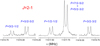 |
Fig. A.2 Laboratory measurements of a section of the rotational spectrum for the CCC33S observed in this work, showing the five hyperfine components for the J=2-1 rotational transition. The spectra were achieved by 200-shots of accumulation. The coaxial arrangement of the adiabatic expansion and the resonator axis in the FTMW spectrometer produces an instrumental Doppler doubling. The resonance frequencies are calculated as the average of the two Doppler components. |
Observed laboratory transition frequencies for CCC33S
Spectroscopic parameters of HCC34S+
Spectroscopic parameters of HC33S+
A.6 HC33S+
To the best of our knowledge the rotational spectrum for the HC33S+ species has not been observed in the laboratory. The rotational constant for the vibrational ground state of this isotopologue can be estimated from the substitution structure provided by Margulès et al. (2003) for the HCS+ molecule to be 21160.0±0.5 MHz. The uncertainty has been estimated from the observed differences between observed and predicted rotational constants for the other isotopologues of HCS+. Using this value as a starting point we easily measured in our line surveys eight hyperfine components of the rotational transitions J=1-0 and 2-1 of HC33S+ (see Fig. 4). The measured frequencies are given in Table B.1. We use the same Hamiltonian and identical coupling scheme than for CCC33S. The analysis provides the rotational constant and the nuclear quadrupole coupling interaction given in Table A.9. This is the first time that this isotopologue of HCS+ is detected in space.
A.7 C4S
C4S (thiobutatrienylidene) has a ground electronic state 3Σ−, and has been previously detected with the QUIJOTE line survey (Cernicharo et al. 2021c). This species has been observed in the laboratory by Hirahara et al. (1993) and Gordon et al. (2001) and its dipole moment has been derived from ab initio calculations to be 4.03 D (Pascoli & Lavendy 1998). Eight rotational transitions, with N=10 up to 15, have been detected and are shown in Fig. A.3. The derived line parameters are given in Table B.1. The predicted frequencies using the rotational constants derived from the available laboratory data show systematic differences with respect to the observed lines in the QUIJOTE’s domain of up to 70 kHz. Hence, we derive improved rotational constants for this species by fitting the standard Hamiltonian of a 3Σ molecule to the laboratory data and to the observed transitions in TMC-1. The results are given in Table A.10.
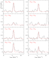 |
Fig. A.3 Observed transitions of C4S observed towards TMC-1. The abscissa corresponds to the local standard of rest velocity of the lines adopting the rest frequencies given in Table B.1. The ordinate corresponds to the antenna temperature corrected for atmospheric and telescope losses in mK. The derived line parameters of the observed lines are given in Table B.1. The synthetic spectra (red line) are derived for N=3.8x1010 cm−2 and the LVG analysis described in section A.7. |
No collisional rate coefficients are available for this species. In order to have an estimation of its excitation we have calculated the C4S-He rate coefficients from the HC3N-He rate coefficients of (Green & Chapman 1978) using the IOS approximation for a 3Σ molecule (Corey 1984; Corey & McCourt 1984; Corey et al. 1986; Fuente et al. 1990). Although these collisional rate coefficients are rather uncertain, they allow us to reproduce reasonably well the observed intensities for a volume density of 4×104 cm−3 (see Fig. A.3). This value of n(H2) has been considered with caution. The calculated excitation temperatures between 31 GHz and 50 GHz vary between 6.5 K and 8 K. The column density for this species is 3.8×1010 cm−2. A similar value can be obtained adopting LTE for a rotational temperature of 8 K. The CCCS/CCCCS abundance ratio of ~180 is consistent with the value derived by Cernicharo et al. (2021c), but much lower than that of CCS/CCCS (~5). The expected line intensities of the isotopologues of C4S are too low to be detected with the present sensitivity of our line survey.
A.8 C5S
C5S (thiopentatetraenylidene) has a ground electronic state 1Σ+. This molecule was first tentatively detected towards IRC +10216 by Bell et al. (1993) and confirmed later by Agúndez et al. (2014) in the same source. It has been also previously detected towards TMC-1 (Cernicharo et al. 2021c). The molecule has been observed in the laboratory up to Ju=10 by (Kasai et al. 1993; Gordon et al. 2001). Laboratory data for all its singly substituted isotopologues are also available (Gordon et al. 2001). The dipole moment of the molecule has been calculated to be 4.65 D by Lee (1997). An inspection of the QUIJOTE data permits to detect all lines of this species between Ju=17 and 26. The observed lines are shown in Fig. A.4 and the derived line parameters are given in Table B.1. Some systematic frequency differences are found between observed and predicted frequencies. Hence, improved rotational constants are provided in Table A.11 which have been obtained from a fit to the laboratory and space frequencies using the standard Hamiltonian for a linear molecule.
Spectroscopic parameters of C4S
Spectroscopic parameters of C5S
Collisional rate coefficients for C5S with He have been calculated by Khadri et al. (2020). Using this data, we derive from a fit to the observed line profiles a value for the density of H2 of 5×104 cm−3 and a column density for C5S of 3.0×1010 cm−2. Similar column densities are obtained for an uniform rotational temperature of 8.5 K. Hence, it seems that C4S and C5S have similar abundances.
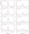 |
Fig. A.4 Observed transitions of C5S observed towards TMC-1. The abscissa corresponds to the local standard of rest velocity of the lines adopting the rest frequencies given in Table B.1. The ordinate corresponds to the antenna temperature corrected for atmospheric and telescope losses in mK. The derived line parameters of the observed lines are given in Table B.1. The synthetic spectra (red line) are derived for N=3.0x1010 cm−2 and the LVG analysis described in section A.8. |
References
- Agúndez, M., Fonfría, J. P., Cernicharo, J., et al. 2008, A&A, 479, 493 [NASA ADS] [CrossRef] [EDP Sciences] [Google Scholar]
- Agúndez, M., Cernicharo, J., & Guélin, M. 2014, A&A, 570, A45 [Google Scholar]
- Agúndez, M., Cernicharo, J., de Vicente, P., et al. 2015, A&A, 579, L10 [Google Scholar]
- Agúndez, M., Marcelino, N., Cernicharo, J., et al. 2019, A&A, 625, A147 [NASA ADS] [CrossRef] [EDP Sciences] [Google Scholar]
- Agúndez, M., Cabezas, C., Marcelino, N., et al. 2022, A&A, 659, L9 [NASA ADS] [CrossRef] [EDP Sciences] [Google Scholar]
- Agúndez, M., Marcelino, N., Tercero, B., et al. 2023, A&A, 677, A106 [NASA ADS] [CrossRef] [EDP Sciences] [Google Scholar]
- Agundez, M., Molpeceres, G., Cabezas, C., et al. 2025, A&A, 693, L20 [NASA ADS] [CrossRef] [EDP Sciences] [Google Scholar]
- Ahrens, V., & Winnewisser, G. 1999, Z. Naturforsch, 54a, 131 [Google Scholar]
- Anders, E., & Grevesse, N. 1989, Geochim. Cosmochim. Acta, 53, 197 [Google Scholar]
- Bell, M. B., Avery, L. W., & Feldman, P. A. 1993, ApJ, 417, L37 [Google Scholar]
- Bogey, M., Demuynch, C., & Destombes, J. L. 1981, Chem. Phys. Lett., 81, 256 [NASA ADS] [CrossRef] [Google Scholar]
- Bogey, M., Demuynch, C., & Destombes, J. L. 1982, J. Mol. Spectrosc., 95, 35 [Google Scholar]
- Bogey, M., Demuynch, C., Destombes, J. L., & Lemoine, B. 1984, J. Mol. Spectrosc., 107, 417 [Google Scholar]
- Botchswina, P., & Sebald, P. 1985, J. Mol. Spectrosc., 110, 1 [Google Scholar]
- Burkholder, J. B., Lovejoy, E. R., Hammer, P. D., & Howard, C. J. 1987, J. Mol. Spectrosc., 124, 450 [Google Scholar]
- Cabezas, C., Guillemin, J.-C., & Endo, Y. 2016, J. Chem. Phys., 145, 184304 [Google Scholar]
- Cabezas, C., Roueff, E., Tercero, B., et al. 2021, A&A, 650, L15 [NASA ADS] [CrossRef] [EDP Sciences] [Google Scholar]
- Cabezas, C., Fuentetaja, R., Roueff, E., et al. 2022a, A&A, 657, L5 [NASA ADS] [CrossRef] [EDP Sciences] [Google Scholar]
- Cabezas, C., Agúndez, M., Marcelino, N., et al. 2022b, A&A, 657, L4 [NASA ADS] [CrossRef] [EDP Sciences] [Google Scholar]
- Cabezas, C., Agúndez, M., Endo, Y., et al. 2024, A&A, 686, L3 [NASA ADS] [CrossRef] [EDP Sciences] [Google Scholar]
- Cernicharo, J. 1985, Internal IRAM report (Granada: IRAM) [Google Scholar]
- Cernicharo, J., 2012, in ECLA 2011: Proc. of the European Conference on Laboratory Astrophysics, EAS Publications Series, eds. C. Stehl, C. Joblin, & L. d’Hendecourt (Cambridge: Cambridge University Press), 251 [Google Scholar]
- Cernicharo, J., & Guélin, M. 1987, A&A, 176, 299 [Google Scholar]
- Cernicharo, J., Guélin, M., Hein, H., & Kahane, C. 1987, A&A, 181, L9 [Google Scholar]
- Cernicharo, J., Marcelino, N., Rouef, E., et al. 2012, ApJ, 759, L43 [Google Scholar]
- Cernicharo, J., Marcelino, N., Agúndez, et al. 2020, A&A, 642, L8 [NASA ADS] [CrossRef] [EDP Sciences] [Google Scholar]
- Cernicharo, J., Agúndez, M., Kaiser, R. et al. 2021a, A&A, 652, L9 [NASA ADS] [CrossRef] [EDP Sciences] [Google Scholar]
- Cernicharo, J., Agúndez, M., Cabezas, C., et al. 2021b, A&A, 649, L15 [EDP Sciences] [Google Scholar]
- Cernicharo, J., Agúndez, M., Kaiser, R. I., et al. 2021c, A&A, 655, L1 [NASA ADS] [CrossRef] [EDP Sciences] [Google Scholar]
- Cernicharo, J., Cabezas, C., Agúndez, M., et al. 2021d, A&A, 648, L3 [EDP Sciences] [Google Scholar]
- Cernicharo, J., Cabezas, C., Endo, Y., et al. 2021e, A&A, 650, L14 [NASA ADS] [CrossRef] [EDP Sciences] [Google Scholar]
- Cernicharo, J., Cabezas, C., Endo, Y., et al. 2021f, A&A, 646, L3 [EDP Sciences] [Google Scholar]
- Cernicharo, J., Tercero, B., Marcelino, N., et al. 2023, A&A, 674, L4 [NASA ADS] [CrossRef] [EDP Sciences] [Google Scholar]
- Cernicharo, J., Tercero, B., Cabezas, C. et al. 2024a, A&A, 682, L13 [NASA ADS] [CrossRef] [EDP Sciences] [Google Scholar]
- Cernicharo, J., Agúndez, M., Cabezas, C., et al. 2024c, A&A, 682, L4 [NASA ADS] [CrossRef] [EDP Sciences] [Google Scholar]
- Chin, Y.-N., Henkel, C., Whiteoak, J. B., et al. 1996, A&A, 305, 960 [NASA ADS] [Google Scholar]
- Colzi, L., Sipilä, O., Roueff, E., et al. 2020, A&A, 640, A51 [NASA ADS] [CrossRef] [EDP Sciences] [Google Scholar]
- Corey, G. C. 1984, J. Chem. Phys., 81, 2678 [CrossRef] [Google Scholar]
- Corey, G. C., & McCourt, F.R. 1984, J. Chem. Phys., 84, 2723 [Google Scholar]
- Corey, G. C. Alexander, M. H. & Schaefer, J. 1986, J. Chem. Phys., 85, 2726 [Google Scholar]
- Denis-Alpizar, O., Stoecklin, T., Guilloteau, S., et al. 2018, MNRAS, 478, 1811 [Google Scholar]
- Denis-Alpizar, O., Quintas-Sánchez, E., & Dawes. R. 2022, MNRAS, 512, 5546 [NASA ADS] [CrossRef] [Google Scholar]
- Dunning, T. H., 1989, J. Chem. Phys. 90, 1007 [Google Scholar]
- Endo, Y., Kohguchi, H., Ohshima, Y. 1994, Faraday Discuss., 97, 341 [Google Scholar]
- Faure, A., Lique, F., & Wiesenfeld, L. 2016, MNRAS, 460, 2103 [NASA ADS] [CrossRef] [Google Scholar]
- Fehèr, O., Tóth, L.V., Ward-Thompson, D. et al. 2016, A&A, 590, A75 [Google Scholar]
- Flower, D. R., & Lique, F. 2015, MNRAS, 446, 1750 [NASA ADS] [CrossRef] [Google Scholar]
- Fossé, D., Cernicharo, J., Gerin, M., & Cox, P. 2001, ApJ, 552, 168 [Google Scholar]
- Frisch, M. J., Trucks, G. W., Schlegel, H. B., et al. 2016, Gaussian 16 Revision A.03 [Google Scholar]
- Fuente, A., Cernicharo, J., Barcia, A., & Gómez-Gónzalez, J. 1990, A&A, 231, 151 [Google Scholar]
- Fuente, A., Navarro, D. G., Caselli, P., et al. 2019, A&A, 624, A105 [NASA ADS] [CrossRef] [EDP Sciences] [Google Scholar]
- Fuente, A., Rivière-Marichalar, P., Beitia-Antero, L., et al. 2023, A&A, 670, A114 [NASA ADS] [CrossRef] [EDP Sciences] [Google Scholar]
- Fuentetaja, R., Agúndez, M., Cabezas, C., et al. 2022, A&A, 667, L4 [NASA ADS] [CrossRef] [EDP Sciences] [Google Scholar]
- Furuya, K., Aikawa, Y., Sakai, N., et al. 2011, ApJ, 731, 38 [Google Scholar]
- Godard Palluet, A., & Lique., F. 2023, J. Chem. Phys., 158, 044303 [Google Scholar]
- Godard Palluet, A., & Lique, F. 2024, MNRAS, 527, 6702 [Google Scholar]
- Gordon, V. D., McCarthy, M. C., Apponi, A. J., et al. 2001, ApJS, 134, 311 [NASA ADS] [CrossRef] [Google Scholar]
- Goldreich, P., & Kwan, J. 1974, ApJ, 189, 441 [CrossRef] [Google Scholar]
- Gottlieb, C. A., Myers, P. C., & Thaddeus, P. 2003, ApJ, 588, 655 [NASA ADS] [CrossRef] [Google Scholar]
- Gudeman, C. S., Haese, N. N., Piltch, N. D., & Woods, R. C. 1981, ApJ, 246, L47 [NASA ADS] [CrossRef] [Google Scholar]
- Green, S. 1991, ApJS, 76, 979 [NASA ADS] [CrossRef] [Google Scholar]
- Green, S., & Chapman, S. 1978, ApJS, 37, 169 [Google Scholar]
- Hirahara, Y., Ohshima, Y., & Endo, Y. 1993, ApJ, 408, L113 [NASA ADS] [CrossRef] [Google Scholar]
- Ikeda, M., Sekimoto, Y., & Yamamoto, S. 1997, J. Mol. Spectrosc., 185, 21 [Google Scholar]
- Kaifu, N., Suzuki, H., Ohishi, M., et al. 1987, ApJ, 317, L111 [NASA ADS] [CrossRef] [Google Scholar]
- Kaifu, N., Ohishi, M., Kawaguchi, K., et al. 2004, PASJ, 56, 69 [Google Scholar]
- Kasai, Y., Obi, K., Ohshima, Y. et al. 1993, ApJ, 410, L45 [Google Scholar]
- Khadri, F., Chefai, A., & Hammami, K. 2020, MNRAS, 498, 5159 [NASA ADS] [CrossRef] [Google Scholar]
- Kim, E., & Yamamoto, S. 2003, J. Mol. Spectrosc., 219, 296 [Google Scholar]
- Kirk, J. M., Ward-Thompson, D., Palmeirim, P., et al. 2013, MNRAS, 432, 1424 [Google Scholar]
- Lee, S., 1997, Chem. Phys., 268, 69 [Google Scholar]
- Loison, J.-C., Wakelam, V., Gratier, P., et al. 2020, MNRAS, 498, 4663 [NASA ADS] [CrossRef] [Google Scholar]
- Lovas, F. J., Suenram, R. D., Ogata, T., & Yamamoto, S. 1992, ApJ, 399, 325 [CrossRef] [Google Scholar]
- Lucas, R., & Liszt, H. 1998, A&A, 337, 246 [NASA ADS] [Google Scholar]
- Margulès, L., Lewen, F., Winnewisser, G., et al. 2003, Phys. Chem. Chem. Phys., 5, 2770 [CrossRef] [Google Scholar]
- McGuire, B. A., Martin-Drumel, M.-A., Lee, K. L. K., et al. 2018b, PCCP, 20, 13870 [Google Scholar]
- Milam, S. N., Savage, C., Brewster, M. A., et al. 2005, ApJ, 634, 1126 [Google Scholar]
- Møller, C., & Plesset, M. S. 1934, Phys. Rev., 46, 618 [Google Scholar]
- Müller, H. S. P., Schlöder, F., Stutzki, J., & Winnewisser, G. 2005, J. Mol. Struct., 742, 215 [Google Scholar]
- Navarro-Almaida, D., Le Gal, R., Fuente, A., et al. 2020, A&A, 637, A39 [NASA ADS] [CrossRef] [EDP Sciences] [Google Scholar]
- Navarro-Almaida, D., Bop, C. T., Lique, F., et al. 2023, A&A, 670, A110 [NASA ADS] [CrossRef] [EDP Sciences] [Google Scholar]
- Ohshima, Y., & Endo, Y. 1992, J. Mol. Spectrosc., 153, 627 [Google Scholar]
- Pardo, J. R., Cernicharo, J., & Serabyn, E. 2001, IEEE Trans. Antennas Propag., 49, 12 [Google Scholar]
- Pascoli, G., & Lavendy, H. 1998, Int. J. Mass Spectrom., 181, 11 [Google Scholar]
- Pickett, H. M. 1991, J. Mol. Spectrosc., 148, 371 [Google Scholar]
- Pickett, H. M., Poynter, R. L., Cohen, E. A., et al. 1998, J. Quant. Spectrosc. Radiat. Transfer, 60, 883 [Google Scholar]
- Ram, R. S., Bernath, P. F., & Davies, S. P. 1995, J. Mol. Spectrosc., 173, 146 [Google Scholar]
- Ritchey, A. M., Federman, S. R., & Lambert, D. L. 2011, ApJ, 728, 36 [NASA ADS] [CrossRef] [Google Scholar]
- Roueff, E., Loison, J.-C., & Hickson, K. M. 2015, A&A, 576, A99 [NASA ADS] [CrossRef] [EDP Sciences] [Google Scholar]
- Sahnoun, E., Ben Khalifa, M., Khadri, F., et al. 2020, Ap&SS, 365, 183 [Google Scholar]
- Saito, S., Kawaguchi, K., Yamamoto, S., et al. 1987, ApJ, 317, L115 [NASA ADS] [CrossRef] [Google Scholar]
- Sakai, N., Ikeda, M., Morita, M., et al. 2007, ApJ, 663, 1174 [Google Scholar]
- Sakai, N., Takano, S., Sakai, S., et al. 2013, J. Phys. Chem., A117, 9831 [Google Scholar]
- Sheffer, Y., Rogers, M., Federman, S. R., et al. 2007, ApJ, 667, 1002 [NASA ADS] [CrossRef] [Google Scholar]
- Stahl, O., Casassus, S., & Wilson, T. 2008, A&A, 477, 865 [NASA ADS] [CrossRef] [EDP Sciences] [Google Scholar]
- Suenram, R. D., Lovas, F. J., et al. 1994, ApJ, 429, L89 [NASA ADS] [CrossRef] [Google Scholar]
- Suzuki, H., Kaifu, N., Miyaji, T., et al. 1984, ApJ, 282, 197 [Google Scholar]
- Takano, S., Masuda, A., Hirahara, Y., et al. 1998, A&A, 329, 1156 [NASA ADS] [Google Scholar]
- Talbi, D., 2018, Austr. J. Chem. 71, 311 [Google Scholar]
- Tang, J., & Saito, S. 1995, Phys. Chem. Chem. Phys., 5, 2770 [Google Scholar]
- Tercero, F., López-Pérez, J. A., Gallego, et al. 2021, A&A, 645, A37 [NASA ADS] [CrossRef] [EDP Sciences] [Google Scholar]
- Tercero, B., Marcelino, N., Agúndez, M., et al. 2024, A&A, 682, L12 [NASA ADS] [CrossRef] [EDP Sciences] [Google Scholar]
- Thaddeus, P., Guélin, M., & Linke, R. A. 1981, ApJ, 246, L41 [NASA ADS] [CrossRef] [Google Scholar]
- Todd, T. T. 1977, J. Mol. Spectrosc., 66, 162 [Google Scholar]
- Todd, T. T., & Olson W. B. 1979, J. Mol. Spectrosc., 74, 190 [Google Scholar]
- Troscompt, N., Faure, A., Wiesenfeld, L., et al. 2009, A&A, 493, 687 [NASA ADS] [CrossRef] [EDP Sciences] [Google Scholar]
- Uehara, H., Horiai, K., & Sakamoto, Y. 2015, J. Mol. Spectrosc., 313, 19 [Google Scholar]
- Wilson, T. L. 1999, Rep. Progr. Phys., 62, 143 [CrossRef] [Google Scholar]
- Winkel, R. J., Davies, S. P., Pecumer R., & Brault, J. W. 1984, Can. J. Phys., 62, 1414 [Google Scholar]
- Winnewisser, G., & Cook, R. L. 1968, J. Mol. Spectrosc., 28, 266 [Google Scholar]
- Yamamoto, S., Saito, S., Kawaguchi, K., et al. 1987, ApJ, 317, L119 [Google Scholar]
- Yamamoto, S., Saito, S., Kawaguchi, K., et al. 1990, ApJ, 361, 318 [NASA ADS] [CrossRef] [Google Scholar]
- Yan, Y. T., Henkel, C., Kobayashi, C. et al. 2023, A&A, 670, A98 [NASA ADS] [CrossRef] [EDP Sciences] [Google Scholar]
Q-band Ultrasensitive Inspection Journey to the Obscure TMC-1 Environment.
All Tables
All Figures
|
Fig. 1 Spatial distribution over a region of 264″×264″ of the integrated-intensity emission of the J=1–0 and J=2–1 transitions (left and right panels, respectively) of CS, C34S, 13CS, and HCS+ (from top to bottom). For each map, the integrated-line emission has been normalized to its maximum value (M). The value of M in mK km s−1 is indicated below the name of the molecule at the top left side of each panel. The HPBW of the telescope for each transition is indicated by the red circle. The central position of the map, corresponding to TMC-1(CP), is indicated by a black dot. |
| In the text | |
|
Fig. 2 Same as Fig. 1, but for the integrated-intensity emission, normalized to M, of several transitions of CCS (left panels), CC34S (two upper right panels) and CCCS (remaining right panels). The value of the maximum integrated intensity (in mK km s−1) is shown at the top left side of each panel. The HPBW of the telescope for each transition is indicated by the red circle. The central position of the map, corresponding to TMC-1(CP), is indicated by a black dot. |
| In the text | |
|
Fig. 3 Observed J = 1–0 and 2–1 lines of CS and its isotopologues 13CS, C34S, C33S, and 13C34S toward TMC-1. For C36S and 13C33S, only the J=1–0 line was detected. The abscissa corresponds to the local standard of rest velocity of the lines adopting the rest frequencies given in Table B.1. In the two bottom panel, however, the abscissa corresponds to the rest frequency. The ordinate corresponds to the antenna temperature corrected for atmospheric and telescope losses in mK. The derived line parameters for the observed lines are given in Table B.1. The synthetic spectra (red line) are derived for the column densities shown in Table 1 and the LVG model described in Sections 3 and 4.1. For CS, a two-layer component model is used (see Section 4.1). Negative features appearing in the folding of the frequency switching data are blanked in all the figures. The observed spectrum of the hyperfine component J=1–0, F=1/2–3/2 of C33S was multiplied by 0.1. |
| In the text | |
|
Fig. 4 Observed J = 1–0 and 2–1 lines of HCS+ and its isotopologues towards TMC-1. The abscissa corresponds to the local standard of rest velocity of the lines adopting the rest frequencies given in Table B.1. The bottom panels show the same transitions of HC33S+, which exhibit several hyperfine components. The abscissa in this case is the rest frequency adopting a velocity for the source of 5.83 km s−1 (Cernicharo et al. 2020). The ordinate corresponds to the antenna temperature corrected for atmospheric and telescope losses in mK. The derived line parameters for the observed lines are given in Table B.1. The synthetic spectra (red line) are derived for the column densities shown in Table 1 and the LVG model described in Sections 3 and 4.2. |
| In the text | |
|
Fig. 5 Observed lines of CCS towards TMC-1. The abscissa corresponds to the local standard of rest velocity of the lines adopting the rest frequencies given in Table B.1. The ordinate corresponds to the antenna temperature corrected for atmospheric and telescope losses in mK. The derived line parameters are given in Table B.1. The synthetic spectra (red line) are derived for the column densities shown in Table 1 and the LVG model described in Section 3 with n(H2)=1.3×104 cm−3 and N(CCS)=3.4×1013 cm−2 (see Section 4.3). |
| In the text | |
|
Fig. 6 Observed lines of CC34S towards TMC-1. The abscissa corresponds to the local standard of rest velocity of the lines adopting the rest frequencies given in Table B.1. The ordinate corresponds to the antenna temperature corrected for atmospheric and telescope losses in mK. The derived line parameters are given in Table B.1. The synthetic spectra (red line) are derived from the LVG model described in Section 3 with n(H2)=1.3×104 cm−3 and N(CC34S)=1.5×1012 cm−2 (see Section 4.3). |
| In the text | |
|
Fig. 7 Observed hyperfine components of the NJ = 23−12 (left panels) and NJ = 34–23 (right panels) transitions of 13CCS, C13CS, and C13C34S towards TMC-1. The abscissa corresponds to the rest frequency in MHz. The ordinate corresponds to the antenna temperature corrected for atmospheric and telescope losses in mK. The derived line parameters are given in Table B.1. The synthetic spectra (red line) are derived from the LVG model described in Section 3 with n(H2)=1.3×104 cm−3 and the column densities given in Table 1 (see Section 4.3). |
| In the text | |
|
Fig. 8 Observed hyperfine components of the NJ = 23−12 (upper panels) and NJ = 34–23 (bottom panels) transitions of CC33S towards TMC-1. The derived line parameters of the observed lines are given in Table B.1. The abscissa corresponds to the rest frequency in MHz. The ordinate corresponds to the antenna temperature corrected for atmospheric and telescope losses in mK. The synthetic spectra (red line) are derived from the LVG model described in Section 3 with n(H2)=1.3×104 cm−3 and N(CC33S)=3.5×1011 cm−2 (see Section 4.3). |
| In the text | |
|
Fig. 9 Observed transitions of CCCS, CCC34S, 13CCCS, and C13CCS towards TMC-1. All transitions of CCCS are shown in the left panels. The right panels show J=6–5, 7–6, and 8–7 of the three isotopologues. The abscissa corresponds to the local standard of rest velocity of the lines adopting the rest frequencies given in Table B.1. The ordinate corresponds to the antenna temperature corrected for atmospheric and telescope losses in mK. The derived line parameters are given in Table B.1. The synthetic spectra (red lines) have been calculated from the LVG model described in Section 4.4. The adopted volume density is n(H2)=1.3×104 cm−3 for all isotopologues, and the resulting column densities are given in Table 1. |
| In the text | |
|
Fig. 10 Observed transitions of CCC33S towards TMC-1. The abscissa corresponds to the rest frequency. The ordinate corresponds to the antenna temperature corrected for atmospheric and telescope losses in mK. The derived line parameters are given in Table B.1. The synthetic spectra (red line) are derived from a model with N=6.2x1010 cm−2 and Trot=8 K (see Section 4.4). |
| In the text | |
|
Fig. 11 Observed transitions of H2CS and its isotopologues towards TMC-1. The abscissa corresponds to the local standard of rest velocity of the lines adopting the rest frequencies given in Table B.1, except for the bottom panel (H2C33S) for which it corresponds to the rest frequency. The ordinate corresponds to the antenna temperature corrected for atmospheric and telescope losses in mK. The derived line parameters are given in Table B.1. The synthetic spectra (red line) are derived from the LVG model described in Section 4.5. The modelled spectra for the 313−212 transition of H2CS, H2C34S and H213CS have been multiplied by a correction factor indicated in blue at the top right side of the corresponding panels. For all the other transitions, no correction factors are applied. This factor results from the adopted collisional rate coefficients for H2CS (see Section 4.5). |
| In the text | |
|
Fig. 12 Observed lines of HCC34S+ towards TMC-1. The abscissa corresponds to the rest frequency. The ordinate corresponds to the antenna temperature corrected for atmospheric and telescope losses in mK. The derived line parameters of the observed lines are given in Table B.1. The modelled spectra (red line) are derived for N(HCC34S+)=4.7×1010 cm−2 adopting the kinetic temperatures calculated for CC34S as the rotational temperature for n(H2)=1.3×104 cm−3. |
| In the text | |
|
Fig. A.1 Laboratory measurements of the three hyperfine components of the NJ=21−10 rotational transition of CC33S we observed. The abscissa corresponds to the frequency of the lines in MHz. The spectra were achieved by 100-shots of accumulation. The coaxial arrangement of the adiabatic expansion and the resonator axis in the FTMW spectrometer produces an instrumental Doppler doubling. The resonance frequencies are calculated as the average of the two Doppler components. |
| In the text | |
|
Fig. A.2 Laboratory measurements of a section of the rotational spectrum for the CCC33S observed in this work, showing the five hyperfine components for the J=2-1 rotational transition. The spectra were achieved by 200-shots of accumulation. The coaxial arrangement of the adiabatic expansion and the resonator axis in the FTMW spectrometer produces an instrumental Doppler doubling. The resonance frequencies are calculated as the average of the two Doppler components. |
| In the text | |
|
Fig. A.3 Observed transitions of C4S observed towards TMC-1. The abscissa corresponds to the local standard of rest velocity of the lines adopting the rest frequencies given in Table B.1. The ordinate corresponds to the antenna temperature corrected for atmospheric and telescope losses in mK. The derived line parameters of the observed lines are given in Table B.1. The synthetic spectra (red line) are derived for N=3.8x1010 cm−2 and the LVG analysis described in section A.7. |
| In the text | |
|
Fig. A.4 Observed transitions of C5S observed towards TMC-1. The abscissa corresponds to the local standard of rest velocity of the lines adopting the rest frequencies given in Table B.1. The ordinate corresponds to the antenna temperature corrected for atmospheric and telescope losses in mK. The derived line parameters of the observed lines are given in Table B.1. The synthetic spectra (red line) are derived for N=3.0x1010 cm−2 and the LVG analysis described in section A.8. |
| In the text | |
Current usage metrics show cumulative count of Article Views (full-text article views including HTML views, PDF and ePub downloads, according to the available data) and Abstracts Views on Vision4Press platform.
Data correspond to usage on the plateform after 2015. The current usage metrics is available 48-96 hours after online publication and is updated daily on week days.
Initial download of the metrics may take a while.