| Issue |
A&A
Volume 702, October 2025
|
|
|---|---|---|
| Article Number | A186 | |
| Number of page(s) | 15 | |
| Section | Extragalactic astronomy | |
| DOI | https://doi.org/10.1051/0004-6361/202554400 | |
| Published online | 20 October 2025 | |
A3COSMOS: The dust content of massive quiescent galaxies and its evolution with cosmic time
1
Argelander-Institut für Astronomie, Universität Bonn, Auf dem Hügel 71, 53121
Bonn, Germany
2
Université Paris-Saclay, Université Paris Cité, CEA, CNRS, AIM, 91191
Gif-sur-Yvette, France
3
Aix Marseille Univ, CNRS, CNES, LAM, Marseille, France
4
Purple Mountain Observatory, Chinese Academy of Sciences, 10 Yuanhua Road, Nanjing, 210023, China
5
Max Planck Institute for Astronomy, Königstuhl 17, D-69117, Germany
⋆ Corresponding author: This email address is being protected from spambots. You need JavaScript enabled to view it.
Received:
6
March
2025
Accepted:
18
August
2025
Abstract
Aims. We study the dust content of massive (log(M*/M⊙)≥10.8) quiescent galaxies (QGs) at redshifts z = 0.5 − 3 to place constraints on the evolution of their cold interstellar medium (ISM) and thereby obtain insights into the processes of galaxy quenching throughout cosmic time.
Methods. We used a robust sample of 458 colour-selected QGs covered by the A3COSMOS+A3GOODSS database to perform a stacking analysis in the uv domain and measured their mean dust masses from their stacked sub-millimetre luminosities. We used the CIGALE spectral energy distribution fitting code to obtain star formation histories and infer the time since quenching for all the QGs in our sample. We used this information to gain insight into the time evolution of the dust content after quenching.
Results. Most QGs in our sample quenched around a redshift of z ∼ 1.3, following the peak of cosmic star formation. The majority of QGs observed at z > 1 are recently quenched (i.e. quenched for no longer than 500 Myr), whereas the majority of QGs observed at z < 1 have already been quenched for a significant amount of time (≳1 Gyr). This implies that high-redshift galaxies (z ≳ 2) are ideal for studying the mechanisms of quenching and its effects on the ISM, while lower-redshift galaxies are more suitable for studying the long-term effects of the QG environment on their ISM. We obtain upper limits on the dust mass fraction of the QG population that indicate a lower dust content in high-redshift massive QGs than what was found by earlier stacking studies, and significantly lower (by a factor of ∼2–6) than that of normal star-forming galaxies. We also place constraints on the initial gas fraction right after quenching. We find that within the first ∼600 Myr after quenching, QGs already lose on average ≳70% of their cold ISM. Our findings support a gas consumption or removal scenario acting on short timescales.
Key words: galaxies: evolution / galaxies: high-redshift / galaxies: ISM / submillimeter: ISM
© The Authors 2025
 Open Access article, published by EDP Sciences, under the terms of the Creative Commons Attribution License (https://creativecommons.org/licenses/by/4.0), which permits unrestricted use, distribution, and reproduction in any medium, provided the original work is properly cited.
This article is published in open access under the Subscribe to Open model. This email address is being protected from spambots. You need JavaScript enabled to view it. to support open access publication.
1. Introduction
It has been known for many years that galaxies constitute a distinctly bimodal population that can be observed from the local Universe out to at least cosmic noon (z ∼ 2; e.g. Williams et al. 2009; Wuyts et al. 2011). This population is divided into (i) active star-forming galaxies (SFGs), which are disk-dominated systems with young stellar populations that follow a tight relation in the star formation rate (SFR)–stellar mass plane, the so-called main sequence (MS; e.g. Noeske et al. 2007; Speagle et al. 2014; Schreiber et al. 2015; Popesso et al. 2023; Koprowski et al. 2024), and (ii) passive quiescent galaxies (QGs), which are bulge-dominated systems with old stellar populations and relatively high stellar masses that are located well below the MS due to very low SFRs. QGs can have high stellar masses of log(M*/M⊙) > 11. To accumulate their stellar mass, they must in the past have been part of the SFG population. The absence of a significant population between SFGs and QGs (this scantly populated transit region is commonly referred to as the ‘green valley’; e.g. Salim 2014) indicates that the transition from the star-forming (SF) phase to quiescence (‘quenching’) must occur on short timescales. The observation of QGs at high redshifts of z ∼ 3 − 7 with the James Webb Space Telescope (JWST; e.g. Valentino et al. 2023; Carnall et al. 2023; de Graaff et al. 2024; Weibel et al. 2024) adds to this conundrum as it poses even more pressingly the question as to how these objects stopped forming stars after assembling high stellar masses within a short cosmic time. Understanding which mechanisms drive the quenching of galaxies is therefore central to the understanding and modelling of galaxy evolution.
The formation of stars is tightly linked to the interstellar medium (ISM) of a galaxy because stars form from clouds of cold molecular gas (e.g. Shu et al. 1987). Quenching must therefore efficiently prevent galaxies from forming stars from their cold gas reservoir, by stabilising the gas against gravitational collapse (morphological quenching; e.g. Martig et al. 2009; Lin et al. 2019; Leśniewska et al. 2023; Michałowski et al. 2024), by dissociating it through heating by active galactic nuclei (AGNs) or stellar feedback (e.g. Conroy et al. 2015; Li et al. 2020; Arjona-Gálvez et al. 2024), or by removing it from the galaxy. Possible mechanisms for the removal of cold gas from a galaxy include ejection through outflows driven by AGNs (e.g. Page et al. 2012; Cicone et al. 2014; Carniani et al. 2016; Belli et al. 2024) or stellar feedback (e.g. Cicone et al. 2014; Hopkins et al. 2014; Dome et al. 2024), and consumption through star formation combined with the prevention of fresh gas accretion (starvation; e.g. Larson et al. 1980; Feldmann & Mayer 2015; Boselli et al. 2016; Trussler et al. 2020). However, it remains unclear as to which of these mechanisms lead to or dominate galaxy quenching throughout cosmic time. To address this question, it is necessary to determine the cold gas content of QGs and the timescales over which it evolves. A commonly used tracer of the cold ISM is the cold dust within it that is observable at far-infrared (FIR) and (sub-)millimetre wavelengths; the latter probes the Rayleigh-Jeans spectral regime.
Quiescent galaxies have very low gas and dust content (e.g. Young et al. 2011; Boselli et al. 2014; Michałowski et al. 2019, 2024; Leśniewska et al. 2023) and are therefore difficult to detect. Furthermore, converting between dust and molecular gas measurements is complicated by the uncertain gas-to-dust ratio (GDR) in QGs. While a GDR of the order of ∼100, corresponding to a typical GDR in SFGs at solar metallicity (e.g. Magdis et al. 2012), is usually assumed, simulations suggest that the GDR in QGs could vary by up to four orders of magnitude (Whitaker et al. 2021a). Despite these limitations, two main approaches exist to study the QG dust emission at high redshifts: (i) deep observations of individual (sometimes lensed) QGs with the Atacama Large Millimeter/submillimeter Array (ALMA; e.g. Bezanson et al. 2019; Williams et al. 2021; Whitaker et al. 2021b; Gobat et al. 2022) and (ii) the stacking of larger samples from wide areas surveys, such as those conducted with Herschel and the James Clerk Maxwell Telescope (JCMT; Gobat et al. 2018; Magdis et al. 2021). These two approaches have led to somewhat conflicting results, with stacking analyses finding dust-to-stellar mass fractions of the order of ∼9 ⋅ 10−4, and the individual observations pointing towards lower dust mass fractions of ≲4 ⋅ 10−4. Blánquez-Sesé et al. (2023) attempted to resolve this discrepancy by stacking a sample of 121 QGs using a selection of observations of the GOODS-South field from the ALMA archive. Their results reduce, but do not resolve, the tension between FIR stacking and individual observations, favouring the FIR stacking results. However, their sample included QGs below the commonly used stellar mass limit of 1010.8 M⊙ and did not take the mass dependence of the dust mass fraction into account. The origin of the tension between the different dust mass estimates thus remains unclear. To address this, it may help to expand the stacking analysis to a larger and mass-matched sample of massive QGs.
In this work we present a stacking analysis of a large and mass-complete sample of colour-selected massive QGs using data from the Automated Mining of the ALMA Archive in the COSMOS and GOODS-South Field (A3COSMOS/A3GOODSS; Liu et al. 2019a; Adscheid et al. 2024), which we used to measure the dust content of high-redshift QGs on a population-wide scale. We supplemented this with measurements of the star formation history (SFH) through spectral energy distribution (SED) fitting using the CIGALE code (Boquien et al. 2019). This provides constraints on the evolution of the dust content after quenching. Thereby we can place the as yet most stringent upper limits on the gas and dust content of massive QGs (M* > 1010.8 M⊙), showing that they lose the bulk of their cold ISM (≳70%) already at the beginning of quiescence (≲600 Myr after quenching).
We present the galaxy selection and ALMA data in Sect. 2. The SED fitting and stacking methods are described in Sect. 3. In Sect. 4 we present and discuss our results, and we summarise our findings in Sect. 5. In the following we assume a flat Λ cold dark matter cosmology with H0 = 70 km s−1 Mpc−1, ΩΛ = 0.7, ΩM = 0.3, and a Salpeter (1955) initial mass function, correcting stellar masses and SFRs where necessary.
2. Data
2.1. ALMA data
For the stacking analysis, we made use of the combined A3COSMOS/A3GOODSS database (data version 20220606; Adscheid et al. 2024). This dataset comprises all observations from the public ALMA archive within the Cosmic Evolution Survey field (COSMOS; Scoville et al. 2007) and Great Observatories Origins Deep Survey Southern field (GOODS-South; Dickinson et al. 2003) publicly available as of 06.06.2022. Calibration of the data was performed using the Common Astronomy Software Application (CASA; McMullin et al. 2007) using the respective scriptforPI.py provided by the ALMA observatory for each project. We used all observations from ALMA bands 3 to 7 (0.8–3.6 mm) conducted in Cycle 3 or later. Projects from earlier cycles had to be excluded, as the definition of the visibility weights assigned during calibration differs between cycles ≥3 and earlier ones, which renders the combination of the visibilities during stacking inaccurate (see Wang et al. 2022). In total, this yields 196 unique projects with 3257 observations. Most of these are in the bands 7 and 6 (1505 and 1055, respectively), followed by bands 3 and 4 (470 and 215), while band 5 contains only a few observations (12). For details on the data, see Liu et al. (2019a) and Adscheid et al. (2024).
2.2. A robust sample of quiescent galaxies
In the following, we describe the process of selecting a robust QG sample within the A3COSMOS/A3GOODSS database. This process is also schematically outlined in Fig. 1.
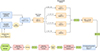 |
Fig. 1. Flow diagram of the selection of a robust QG sample. Blue panels denote general selections, orange panels the selection of QGs, red panels further cleaning steps, and green panels the number of QGs after every step. |
2.2.1. Galaxy catalogues
We selected our sample of QGs from two catalogues: the COSMOS2020 CLASSIC catalogue from Weaver et al. (2022) for the COSMOS field, and the the FOURSTAR galaxy evolution survey (ZFOURGE) catalogue from Straatman et al. (2016) for GOODS-South. Both catalogues provide UV/optical to near-infrared photometry, as well as photometric redshifts and stellar population properties inferred from SED fitting. From these catalogues, we selected galaxies (identified by the flags lp_type = 0 in COSMOS2020 and Use = 1 in ZFOURGE, respectively) in the redshift range z = 0.5 − 3 and with high stellar masses of log(M*/M⊙)≥10.8. This particular mass limit was chosen to be comparable with previous works on massive QGs (e.g. Gobat et al. 2018; Magdis et al. 2021), and was also considered sufficient since, despite the wealth of ALMA observations used, even these massive systems yielded only upper limits in our analysis. In this high mass regime, both the COSMOS2020 CLASSIC and ZFOURGE catalogue are mass-complete (see Straatman et al. 2016; Weaver et al. 2023). Furthermore, this relatively high mass limit of 1010.8 M⊙ also minimises the impact that any potential mass dependence on the dust content of QGs (e.g. Blánquez-Sesé et al. 2023) could have on our results.
In the creation of the catalogues, different SED-fitting codes were used to infer the redshifts and stellar population properties: for COSMOS2020, both properties were inferred using the LePhare code (Arnouts et al. 2002; Ilbert et al. 2006), while for ZFOURGE, the EAZY code (Brammer et al. 2008) was used to obtain the photometric redshifts, and the FAST code (Kriek et al. 2009) was used for the stellar population properties. To ensure that the samples from the two catalogues are combinable, we used the ZFOURGE catalogue available in the COSMOS region of the Cosmic Assembly Near-infrared Deep Extragalactic Legacy Survey (Grogin et al. 2011) and spatially cross-matched it with the COSMOS2020 catalogue (with a matching radius of 1 arcsec) to identify common sources. Restricting this set of common sources to those identified as QGs (38 galaxies; see Sect. 2.2.2), we found very consistent photometric redshifts between these two catalogues (with a median deviation of < 1%) but a small systematic offset between their stellar masses, with those in ZFOURGE being 0.11 dex (median) lower than those in COSMOS2020. We therefore applied a small upward correction of 0.11 dex to the stellar masses of all ZFOURGE galaxies to ensure that the masses in the two catalogues are comparable.
In addition to the photometric information from the COSMOS2020 and ZFOURGE catalogues, we also included mid-infrared (MIR) photometry from Spitzer/Multiband Imaging Photometer for Spitzer (MIPS) 24 μm to obtain a wider photometric coverage for our SED-fitting (see Sect. 3.1). These were taken from the ‘super-deblended’ FIR catalogue of Jin et al. (2018) for COSMOS (1σ ∼ 16 μJy), and from the PEP-GOODS-Herschel catalogue of Magnelli et al. (2013) for GOODS-South (1σ ∼ 7 μJy), which were spatially cross-matched (with a radius of 1 arcsec) with our galaxy sample. Amongst the final 458 galaxies (383 in COSMOS and 75 in GOODS-S) identified as quiescent (see Sects. 2.2.2, 2.2.3, 3.1, and 3.2), 73 (∼16%) are detected in the MIPS 24 μm bands. The properties of these galaxies are specifically discussed in Appendix C.
2.2.2. Quiescent galaxy selection
Quiescent galaxies were selected from the sample of z = 0.5 − 3 and log(M*/M⊙)≥10.8 galaxies defined in the previous section using a series of different colour selection criteria. Following Magdis et al. (2021), we first selected galaxies based on the rest-frame NUV-J-r criterion of Ilbert et al. (2013),
 (1)
(1)
Then, following again Magdis et al. (2021), we applied additional observed-frame colour selections based on the redshift of any given source to further ensure the quiescence of these galaxies. For galaxies at z < 1, we used the B-z-K criterion defined for 0.3 ≤ z < 1.0 galaxies by Magdis et al. (2021):
 (2)
(2)
For 1.0 ≤ z < 1.4 galaxies, we used the r-J-K criterion from Magdis et al. (2021),
 (3)
(3)
For 1.4 ≤ z < 2.5 galaxies, the B-z-K criterion from Daddi et al. (2004),
 (4)
(4)
And for 2.5 < z < 4.0 galaxies, the r-J-L criterion from Daddi et al. (2004):
 (5)
(5)
For the L3.6-band we used the photometry from Spitzer/Infrared Array Camera (IRAC) channel 1, which is centred at 3.55 ± 0.75 μm (IRAC Instrument Team & IRAC Instrument Support Team 2021).
To further ensure the quiescence of the galaxies in our sample, we additionally applied a SFR selection. Galaxies were only kept if their SFR and stellar mass places them at least 0.5 dex below the SF MS at their respective redshift, for which we applied the MS definition of Schreiber et al. (2015). Before cross-matching with the area covered by A3COSMOS/A3GOODSS observations, our sample of robust QGs contains 4583 objects.
We note that some previous works also exclude MIR-detected galaxies from their analyses (e.g. Magdis et al. 2021), while other works include them (e.g. Blánquez-Sesé et al. 2023). We chose to not exclude MIR-detected galaxies a priori to avoid biasing our sample against galaxies containing an AGN. We instead discuss the influence of such an exclusion on our results in Appendix C.
2.2.3. A3COSMOS/A3GOODSS selection
For the purpose of stacking, we kept only the 540 QGs covered by the A3COSMOS/A3GOODSS database, with a primary beam attenuation ≥0.5. We then checked for counterparts of those QGs in the A3COSMOS/A3GOODSS catalogues, finding no such counterparts within the high positional accuracy offered by these two catalogues (σpos ≈ θFWHM/(2 ⋅ S/Npeak); Ball 1975; Condon 1997). This was to be expected from our stringent quiescence selection criteria and the previously reported faint sub-millimetre emission of QGs (e.g. Magdis et al. 2021). In contrast, we found a number of QGs located in the vicinity of A3COSMOS/A3GOODSS detections (supposedly mostly due to projection effects). The emission from these nearby bright sources could significantly impact the faint emission of the QGs we wanted to to study. To mitigate the impact of nearby bright sources on our results, we decided to exclude from our sample (i) all QGs located closer than 3 arcsec to a detected source in the A3COSMOS/A3GOODSS catalogues (i.e. S/Npeak ≥ 4.35 and 5.4 for prior and blindly detected sources, respectively; see Liu et al. 2019a; 24 QGs are excluded with this criterion), and additionally (ii) QGs located closer to a bright source than a minimum distance rmin (49 QGs are excluded with this criterion). This minimum distance was determined from the S/Npeak of the nearby detected source following
 (6)
(6)
The values a and b were empirically calibrated, so that rmin(S/Npeak = 4.35 or 5.4) = 3 arcsec for prior/blindly detected sources, and rmin(S/Npeak = 50) = 10 arcsec. This two-fold selection criterion allowed us to exclude both the directly affected area in the vicinity around these bright sources (within a ∼1–2 FWHM radius) and the wider area still affected by the presence of energetic sidelobes. Through variation of these parameters, we verified that the exact values of these parameters do not significantly influence the results presented in this paper.
The final sample consists of 467 QGs, with a mean observed redshift of ⟨zobs⟩∼1.1. This increases by a factor of ∼4 the number of QGs with ALMA coverage compared to Blánquez-Sesé et al. (2023), who also performed a QG stacking analysis using ALMA data. Many of the ALMA archival data used here are also deeper than in Blánquez-Sesé et al. (2023). The distributions of our A3COSMOS/A3GOODSS-covered sample in stellar mass, redshift, and SFR are very similar to those of the parent sample of 4583 QGs. We verified that the two samples follow the same underlying distributions using two-sample Kolmogorov-Smirnov (KS) tests (p-value > 0.05).
3. Methods
3.1. CIGALE fitting
To gain insight into the SFHs of the QGs in our sample, we fitted their combined UV-to-MIR photometry information with the SED fitting code CIGALE (Boquien et al. 2019). For the SFH, we used the flexible delayed-τ model from Ciesla et al. (2017), tailored to quenched (or bursty) systems:
 (7)
(7)
In this model, the SFR rises and then declines exponentially. At a flexible point in time, tflex, it changes suddenly to a constant value until the time of observation, tobs. The factor rSFR denotes the ratio of the SFR after and before this point in time, and can be smaller, greater, or equal to 1, thus allowing for quenching, bursty, or no sudden events. With that, CIGALE in principle allows both fast and slow quenching: fast quenchers would correspond to galaxies with rSFR < 1 early in their SFH, while slow quenchers would have a largely undisturbed SFH, with the SFR gradually declining with time, slowly moving these systems below the MS.
Following Ciesla et al. (2021), we complemented this SFH module with the stellar population model from Bruzual & Charlot (2003), the dust attenuation model from Charlot & Fall (2000), and the dust emission model from Dale et al. (2014). The input parameters for these models are listed in Table 1. Finally, for each fitted galaxy, CIGALE provides the SFH1 and two sets of stellar population parameters: one obtained with the best-fit SED, and one inferred with a Bayesian-like analysis. In our analysis, we used the Bayesian output parameters, as this avoids degeneracy effects from the discreteness of the input parameters.
Input parameters of the CIGALE module used for SED and SFH fitting of our QG sample.
The galaxies in our sample have a good photometric coverage with on average ∼37 photometric data points. The SED fits from CIGALE are overall very good, with the reduced chi-square χred.2 following a log-normal distribution with μ = −0.1 ± 0.2. Nevertheless, we identified six galaxies as 3σ outliers, that is, galaxies with χred.2 ≳ 3. These sources have in common that, while they are well fitted in the optical wavelength regime, they are not well fit in one or several Spitzer/IRAC MIR bands, hinting at a possible source blending or misassociation. As a high χred.2 indicates large uncertainties on the output parameters, we excluded these galaxies from our analysis. We also identified one source for which CIGALE yields a value of rSFR > 1 (whereas the median rSFR in our sample is 0.005). This source also has mostly low signal-to-noise photometry. As this casts doubt on the quiescent nature of the galaxy, it was also excluded. Thus, in total, seven galaxies were excluded, reducing the sample size to 460.
To ensure the reliability of the galaxy parameters yielded by CIGALE, and especially tq, which we use extensively in Sects. 4.1 and 4.3, we performed a mock analysis, following Ciesla et al. (2021, see also Boquien et al. 2019). It is described in Appendix A. This mock analysis reinforces confidence in the galaxy parameters obtained by CIGALE, and in particular the time since quenching, tq, allowing us to incorporate this property into our scientific analysis.
The properties of the 460 QGs in our A3COSMOS/A3GOODSS sample are displayed in Fig. 2 in comparison to the parent sample of 4583 QGs: rSFR, M*, and tq. We also show ΔMS, at the time of observation (i.e. ΔMSobs) and at the time right before quenching, that is, at tflex = tobs − tq:
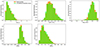 |
Fig. 2. Normalised distribution of CIGALE-inferred Bayesian parameters of the parent sample of 4583 QGs and the 460 QGs in our A3COSMOS/A3GOODSS sample: SFR fraction (rSFR), stellar mass (M*), time since quenching (tq), and (ΔMS) before quenching and at the time of observation. We note that, due to the re-estimation of M* with CIGALE, a small number of galaxies fall slightly below the initial selection threshold of log(M*/M⊙) = 10.8. |
 (8)
(8)
To determine SFRMS(z(tflex),M*(tflex)) at the cosmic time of the quenching event, we used the redshift-dependent MS relation from Schreiber et al. (2015). The redshift of the quenching event, z(tflex), was inferred using the observed redshift of each source and the time since quenching, tq = tobs − tflex, conducting the cosmological calculations with the python package astropy.cosmology (Astropy Collaboration 2013, 2018, 2022). The stellar mass at the time of quenching was computed using tq, SFRobs, and M*(tobs), assuming a return fraction R = 0.27 for a Salpeter (1955) initial mass function (Madau & Dickinson 2014):
 (9)
(9)
Several important conclusions can be drawn from Fig. 2. As per selection the QGs in our sample are massive (log(⟨M*⟩/M⊙)∼11.2). Also, the galaxies in our sample constitute a robust sample of QGs, located well below the MS at the time of observation ( ; interval indicating the 16th and 84th percentiles) and that these systems were, as expected, located around the MS before quenching (
 ). The majority of our QGs have low rSFR, with 99.6% of QGs having rSFR < 0.1, and 71% having rSFR < 0.01, suggesting that our sample is dominated by fast-quenched galaxies. However, the time since quenching, tq, of many QGs in the sample is long (i.e. tq ≳ 1 Gyr) and to conclude that these old systems underwent a rapid quenching event solely on the basis of their low rSFR values could be a misinterpretation. Indeed, while for these systems quenching appears to have begun tq ago relative to their main smoothly evolving SFH component, the CIGALE module is insensitive to gradual evolutions after this point in time. We therefore refrain from making a firm statement about the fraction of fast and slow quenchers in our sample. Finally, we note that the relative distributions of these parameters in our QG sample closely mirror those of the parent sample. In fact, a two-sample KS test on these distributions indicates that our final sample is consistent with being drawn randomly from our parent sample (p-value > 0.05). Hence, reducing the QG sample to the areal coverage of A3COSMOS/A3GOODSS thus does not introduce any significant bias in the analysis of the properties of this population.
3.2. Stacking
To constrain the dust content of our high-redshift, massive QG sample, we performed a stacking analysis in the uv domain using all A3COSMOS/A3GOODSS observations available for them. To this end, we used CASA and the method described in Wang et al. (2022) (see also Wang et al. 2024; Magnelli et al. 2024), to which we refer for the details of the procedure. In the first step, the observed ALMA visibilities of each galaxy were rescaled to rest-frame luminosities at 850 μm,  . This requires prior knowledge of the shape of the IR SED. We therefore used the massive QG SED template of Magdis et al. (2021). The rescaling factor ΓSED is defined as the ratio of the template rest-frame luminosity at 850 μm and at the observed wavelength (Eq. 3 of Wang et al. 2022):
 (10)
(10)
This factor rescales the ALMA visibility amplitudes, |V(u, v, w)|λobs, to 850 μm luminosities using Eq. 4 of Wang et al. (2022):
 (11)
(11)
where DL denotes luminosity distance. The rest-frame wavelengths in our galaxy sample are mostly well in the Rayleigh-Jeans spectral range of the dust continuum (see Appendix D). In this regime, the dust SED is described by a power law depending on the dust spectral emissivity index β, for which Magdis et al. (2021) adopt a value of 1.8. Apart from the chosen β, the rescaling is therefore template-independent. In addition, for each pointing, the phase centre of the rescaled visibilities were shifted to the coordinates of the respective galaxy. The shifted, rescaled visibilities of all galaxies were then concatenated to create one combined measurement set with all galaxies stacked at the phase centre. This combined measurement set was then imaged into the final stack image using the CASA task tclean. The weight of each individual galaxy in the stacked image depends directly on the number of visibilities that correspond to it and on all subsequent conversion factors that were applied to the visibilities (i.e. rest-frame luminosity rescaling, primary beam correction, etc.). Therefore, the relative contribution of a given galaxy to the stack can be easily calculated and is higher for galaxies covered by deeper observations (i.e. many visibilities from one or several ALMA projects), and lower for galaxies covered by shallower observations (i.e. fewer visibilities). Two galaxies had much higher weights (due to long aggregate integration times), and appeared as > 3 σ outliers to the log-normal distribution of galaxy weights in our sample. Their high weights implied that the final stacks were essentially an imprint of only these two sources, which was undesirable, as we aimed to retrieve the mean gas content of the entire population of QGs. We therefore excluded these two galaxies from our analysis, which reduced the total size of our QG sample to 458. As we demonstrate in Appendix B, the individual constraints on the dust content of these two galaxies do not contradict our results, but rather reinforce them, particularly for the more massive system at z ∼ 1.1. Indeed, the dust mass of this system is even below that inferred from stacking for the entire population of QGs.
3.3. Measuring the dust content
We measured the signal in our stacked images (i.e.  ) via an aperture photometry approach. The diameter of the aperture was chosen to be the full width at half maximum of the major axis of the synthesised beam for each stack image, that is, between 0.7 and 1.1 arcsec. The luminosity was measured within the respective aperture at the phase centre of the stack and then divided by the intensity of the point spread function within the same aperture. The uncertainty of the measured luminosity at the image centre was inferred from measurements of luminosities with the same aperture within a radius of ∼8 arcsec from the centre, which is the typical primary beam size in Band 7.
To convert the measured  to dust masses, we used the QG SED template of Magdis et al. (2021), which is normalised to a dust mass of 1.11 ⋅ 108 M⊙. We divided our
  by the 850 μm luminosity of the template to obtain the weighted mean dust mass of the stack in units of 1.11 ⋅ 108 M⊙. We also used the weights of the galaxies in a stack, as defined in Sect. 3.2, to compute the weighted mean stellar mass and redshift of each stack bin. The dust mass inferred using this method naturally depends on the dust temperature assumed by Magdis et al. (2021). QGs generally have distinctly lower dust temperatures than MS galaxies, which typically have dust temperatures of ∼25 − 35 K in our probed redshift range (e.g. Schreiber et al. 2018). If not accounted for, this difference in dust temperature can lead to a significant underestimation of the inferred dust mass (e.g. Cochrane et al. 2022). The QG template of Magdis et al. (2021) therefore assumes a dust temperature of 21 K. We also explore the effect an even lower, yet reasonable dust temperature of 17 K (Cochrane et al. 2022) would have on our results in Sects. 4.2 and 4.3.
4. Results and discussion
4.1. Quenching across cosmic time
In the top panel of Fig. 3, we show the time since quenching, tq, as a function of observed redshift for our QGs in comparison to the parent sample. The distributions of the two samples in this plane are very consistent with one another, with the highest density of galaxies in the range of zobs ≈ 0.5 − 1.5 and tq ≈ 0.5 − 1.5 Gyr. In this diagram, galaxies quenched at the same time (i.e. zq) would fall on a common track, indicated by the solid lines. From these tracks we can identify galaxies that quenched at a similar time and then evolved for a similar period after the end of their SF activity. There are very few galaxies in both samples that quenched at zq > 3, and almost none at zq > 4 (see also the middle panel of Fig. 3). Most QGs in our sample quenched at zq ∼ 0.8 − 2, with a maximum around zq ∼ 1.3. This is in agreement with earlier studies that found the number and mass density of massive QGs to strongly increase between z ∼ 3 and z ∼ 1 and flatten afterwards (e.g. Brammer et al. 2011; Ilbert et al. 2013; Davidzon et al. 2017). This peak in quenching activity closely follows the peak of the cosmic SFR density at z = 1 − 2 (e.g. Ilbert et al. 2013), which suggests a link between these two, with the quenching of these massive systems marking the beginning of the global decline of the cosmic star formation activity. Finally, we note that only ∼17% of QGs in our sample are quenched after zq < 1 and thus at these redshifts, the majority of massive QGs are old.
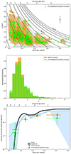 |
Fig. 3. Characterisation of our sample of A3COSMOS/A3GOODSS QGs and the parent sample. Top panel: Time since quenching as a function of the observed redshift. The median error is shown on the right. Solid black lines indicate the locus of galaxies that quenched at the same time, from zq = 0.5 to 5 in steps of 0.5. The orange density map shows the distribution of the parent sample galaxies. The grey shaded areas in the background and dashed grey lines indicate the bins of quenching redshift and time since quenching used in Sect. 4.3. Middle panel: Distribution of quenching redshift (zq). Bottom panel: Fraction of recently quenched galaxies (tq ≤ 500 Myr). The points and horizontal error bars denote the median redshift and the 16th and 84th percentiles of all galaxies in each bin, respectively. The black line shows the fraction of recently quenched massive early-type galaxies as a function of redshift from Gobat et al. (2020). The dotted blue line and shaded area show our toy model based on the stellar mass functions of Davidzon et al. (2017). |
Taken together, all these findings imply that the fraction of recently quenched galaxies within the entire QG population depends on the observed redshift (i.e. zobs), as already pointed out by Gobat et al. (2020). This is clearly demonstrated in the bottom panel of Fig. 3, in which we show the fraction of recently quenched QGs, that is, with tq ≤ 500 Myr, as a function of cosmic time, in our A3COSMOS/A3GOODSS and parent sample. Uncertainties on these fractions were inferred by randomly disturbing the tq parameter of each QG with its error and recomputing the fraction 1000 times. The vertical error bars show the 16th and 84th percentiles of these 1000 realisations, with additional Poisson errors added in quadrature, using the Poisson limits from Gehrels (1986). The A3COSMOS/A3GOODSS and parent samples are fully consistent within their errors. We see a clear increase in the recently quenched fraction by an order of magnitude between zobs ∼ 0.75 and zobs > 1, after which the trend flattens. Our results are in agreement with predictions of Gobat et al. (2020) (based on the evolution of the stellar mass function of massive QGs), except at zobs > 2, where our recently quenched fraction is significantly lower (i.e.  compared to > 0.8). This high-redshift discrepancy could stem from our very conservative selection of QGs, which combines multiple colour criteria with the requirement to be located well below the MS. Our sample could therefore be slightly biased against galaxies that have been quenched very recently, giving us a somewhat limited view of this so-called post-starburst population. However, making our own toy model of the evolution of the fraction of recently quenched galaxies, based on the stellar mass functions of Davidzon et al. (2017), we predicted a slightly lower recently quenched fraction than Gobat et al. (2020) at zobs ≳ 0.75 (by on average ∼28%). These predictions are in good agreement with our observations at zobs < 2, and agree within the uncertainties at zobs ≳ 2 − 3, suggesting that our sample is not strongly biased against galaxies that have been quenched very recently.
4.2. Dust mass fraction
We stacked our QGs in the redshift bins of zobs = 0.5 − 1, 1 − 1.5, 1.5 − 2, and 2 − 3, obtaining stringent 3 σ upper limits on the average dust mass fraction (i.e. Mdust/M*) of the QG population ⟨fdust⟩pop.. The results are listed in Table 2 and shown in Fig. 4 as a function of redshift. Our upper limits yield ⟨fdust⟩pop. ≲ 4 ⋅ 10−4, which is a factor of ∼2 − 7 below the locus of massive MS galaxies2, which indicates that the quiescent nature of these galaxies is associated with a low gas content, rather than solely a low star formation efficiency. These limits are consistent with interferometric measurements of individual massive QGs, in which the dust mass is inferred from either the FIR SED (Whitaker et al. 2021b; Gobat et al. 2022) or CO line measurements (Sargent et al. 2015; Bezanson et al. 2019; Williams et al. 2021). The latter conversion assumes a GDR of 92, which we note is subject to uncertainty (e.g. Whitaker et al. 2021a).
Dust mass fraction inferred from our stacks.
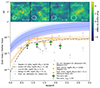 |
Fig. 4. Results of our stacking of four different redshift bins: zobs = 0.5 − 1, 1 − 1.5, 1.5 − 2, and 2 − 3. Top panel: Cutouts of the map centre. We show the profile of the synthesised beam as a dashed white shape in the bottom left, and the number of individual galaxies stacked in the bottom right. The dashed red circle in the centre shows the aperture used to measure the source emission. The colour scaling is set to reflect the signal-to-noise ratio of each pixel. Bottom panel: Dust-to-stellar mass ratio (fdust) of our stacks (green diamonds) at the weighted mean redshift of each stack in comparison to the fdust measurements of massive QGs from the literature; grey symbols show individual measurements from dust (grey hexagons) and CO (grey squares), yellow symbols the results from stacking studies, and the dashed yellow and dash-dotted black lines the predictions from data fitting. The empty diamonds show our upper limits when assuming a lower dust temperature of 17 K. The dashed blue lines and shaded regions show the fdust evolution of massive MS galaxies from Liu et al. (2019b) and Wang et al. (2022). |
These individual measurements are, however, in some tension with population-based results from FIR stacking studies, which find ∼9 ⋅ 10−4 (Gobat et al. 2018; Magdis et al. 2021). To address this issue, Blánquez-Sesé et al. (2023) performed an ALMA stacking study, measuring ⟨fdust⟩pop. slightly lower than Magdis et al. (2021), but agreeing within the errors. However, Blánquez-Sesé et al. (2023) also included galaxies down to stellar masses of log(M*/M⊙) = 10.2, so the compared datasets are not consistent. Indeed, Blánquez-Sesé et al. (2023) support the idea that the gas-to-stellar mass is constant up to log(M*/M⊙)∼11, but decreases rapidly with higher stellar masses. Their ⟨fdust⟩pop. is therefore likely biased high compared to samples of more massive QGs. Our QG selection is consistent with Magdis et al. (2021) (i.e. log(M*/M⊙) > 10.8), yet our measurements are lower by a factor of ∼2 − 3. This is most likely due to the coarser angular resolution of the (sub-)millimetre images stacked by Magdis et al. (2021), who used images from Atacama Submillimeter Telescope Experiment/AzTEC at 1.1 mm and images from JCMT/Submillimetre Common-User Bolometer Array 2 at 850 μm. These instruments have an order of magnitude lower angular resolution than ALMA at the same wavelengths and are hence subject to clustering bias, that is, QGs being located in the same halo as SFGs, and thus not spatially separable in these coarse resolutions. This can introduce a contamination of the measured fluxes with emission from nearby sources, leading to higher dust mass estimates. Although Magdis et al. (2021) consider a clustering contribution to their fluxes, such a posterior separation of emission components is much less precise than avoiding confusion effects from the beginning, as is possible with the excellent angular resolution of ALMA. Naturally, a flux contamination in the measurements of Magdis et al. (2021) implies that their SED template may also be biased. This clustering bias, originating from SFGs with higher dust temperatures than QGs, could indeed lead to greater contamination at shorter than at longer wavelengths. Such contamination may shift the peak of the fitted SED, resulting in a slight overestimation of the dust temperature. However, this effect would somewhat be mitigated by the higher angular resolution of shorter-wavelength observations, which reduces their sensitivity to clustering bias. In any case, even if this differential bias implies that QGs have a lower dust temperature than that assumed in Magdis et al. (2021), our results remain largely unaffected. Indeed, within a reasonable dust temperature range of 17–21 K (Cochrane et al. 2022), (i) our template-based rescaling is mostly insensitive to the assumed dust temperature (see Sect. 3.2), and (ii) adopting a lower temperature of 17 K instead of 21 K would increase our dust mass estimates by only ∼27%, still keeping them below those derived in previous population-based stacking studies.
Our upper limits are only slightly below the trend predicted by the model of Gobat et al. (2020) at z < 2. This model predicts the evolution of the population-wide gas fraction of QGs based on the QG production rate (see the bottom panel of Fig. 3), assuming that QGs start their evolution with a certain initial gas fraction, f0, gas, which decreases exponentially with time:
 (12)
(12)
The model further assumes that f0, gas is a constant fraction of the gas mass of MS galaxies at the time of quenching, Mgas, MS(zq, M*, q): f0, gas = Mgas(tq = 0)/Mgas, MS(zq, M*, q). The model predicts a nearly constant ⟨fdust⟩pop. at z ≳ 1, when the QG population is dominated by recently quenched galaxies, followed by a steep decline of ⟨fdust⟩pop. towards z = 0. At z < 2, where our upper limits are only slightly lower, our fraction of recently quenched galaxies is also largely in agreement with Gobat et al. (2020) (see Fig. 3). At these redshifts, the slight discrepancy between our observations and the model may thus simply arise from a modest bias in the model towards higher f0, gas, introduced during the fitting of the Magdis et al. (2021) data. At z > 2, where our upper limit is a factor of ∼2.5 lower than the model predictions, this discrepancy likely arises from two factors: (i) our sample at this redshift is somewhat biased against recently quenched galaxies (see Sect. 4.1); and (ii) the model likely overestimates f0, gas slightly. To better assess the relative importance of these two effects, we need to explore the dust content as a function of time since quenching, which we do in the following section.
4.3. Dust removal
Dust mass measured from the stacks.
Quiescent galaxies are commonly assumed to lose their gas through an initial short quenching process, followed by a longer phase of declining gas and dust content. As already mentioned, in this framework the parameter f0, gas expresses the gas mass content right after quenching relative to that on the nominal MS. The gradual dust removal in QGs after quenching is generally assumed to follow Eq. 12 with τ ∼ 2.2 − 2.5 Gyr (e.g. Michałowski et al. 2019; Leśniewska et al. 2023; Nadolny et al. 2024). To constrain these two phases of gas removal, we analyse the time evolution of the dust content by (i) grouping galaxies according to their quenching redshift – thereby isolating systems with a similar initial gas removal phase – and (ii) grouping them by time since quenching – capturing galaxies with a consistent after-quenching phase of gas removal. We consider three bins of quenching redshift, zq = 0.75 − 1.25, 1.25 − 1.75, and 1.75 − 2.25, and three bins of time since quenching, tq < 1 Gyr, 1 − 2 Gyr, and 2 − 3 Gyr, as shown in the top panel of Fig. 3. We stacked the QGs in these bins and measured their dust content, obtaining 3 σ upper limits for all stacks. The measured dust masses of the individual stacks are listed in Table 3. Figure 5 shows the dust mass as a function of the time since quenching in relation to the dust mass of MS galaxies at the time of quenching (i.e. Mdust/Mdust, MS(zq, M*, q)), where the dust mass of MS galaxies was inferred from the MS gas-to-stellar mass relation from Wang et al. (2022), converting the molecular gas masses to dust masses using a GDR of 92 (Magdis et al. 2021). Given the low star formation after quenching, rSFR (see Sect. 3.1), we can ignore the stellar mass increase after quenching.
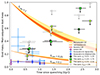 |
Fig. 5. Dust mass at the time of observation divided by the dust mass of MS galaxies at the time of quenching as a function of time since quenching for three different bins of quenching redshift (green filled symbols). The empty symbols show the upper limits when assuming a lower dust temperature of 17 K. The yellow, orange-hatched, and red-chequered regions show the dust removal timescales from Michałowski et al. (2019, τ = 2.5 ± 0.4 Gyr), Leśniewska et al. (2023, τ = 2.26 ± 0.18 Gyr), and Nadolny et al. (2024, τ = 2.28 ± 0.1 Gyr), for three different fractional initial gas fractions (f0, gas). The empty purple symbol marks the f0, gas from the fit of Gobat et al. (2020). Light blue and dark blue symbols show dust mass evolution with time since quenching from Donevski et al. (2023) for spiral and elliptical QGs at z < 0.7, respectively, where we assume a 30% error on the dust mass, and the horizontal error bars denote the bin size of Donevski et al. (2023). |
Figure 5 shows that we can place significant upper limits on the dust mass right after quenching (tq ≲ 1.5 Gyr), whereas at later times, our limits cannot constrain the degenerate parameters f0, gas and τ of the Gobat et al. (2020) model (Eq. 12), although this may be possible in the future. Our results show that after ∼0.6 Gyr, the dust mass is decreased by ≳70%. This is in agreement with the model fitting of Gobat et al. (2020), who inferred a value of  . Our results are also mostly consistent with findings by Donevski et al. (2023) for QGs at z < 0.7.
In SFGs, the accretion of fresh gas from the circumgalactic medium is crucial to maintain a steady star formation activity, balancing gas consumption (e.g. Magnelli et al. 2020; Walter et al. 2020). If gas accretion continues uninterrupted after quenching, we would expect the gas reservoir of QGs to be replenished within the typical gas consumption timescale of SFGs (∼400 − 700 Myr; Walter et al. 2020). Therefore, after the initial drop, Mdust/Mdust, MS should increase back to 1 by tq ∼ 1 − 1.5 Gyr if the accreted gas is not pristine and is mostly falling back onto the galaxy from previous outflow episodes, including the one that led to the current quiescence. However, our upper limits show that Mdust/Mdust, MS is still well below 1 at tq = 1 − 2 Gyr, and even still at tq = 2 − 3 Gyr. This indicates that, if the dominant quenching mechanism operates via gas removal by outflows, the re-accretion of this dust-rich gas onto the galaxy is also efficiently prevented over long periods of time.
Overall, our results thus support that the bulk of the gas and dust reservoir is removed at the beginning of quiescence, and therefore that the loss of most of the gas is necessary for star formation to cease. Larger QG samples will be needed to constrain f0, gas fully, determine whether it evolves with cosmic time, and place constraints on the gas and dust removal timescale.
5. Conclusions
We present an ALMA stacking analysis on a mass-complete sample of 458 QGs with stellar masses > 1010.8 M⊙. We find that most QGs in our sample are quenched between the redshifts z = 1 and 2, following the peak of cosmic SFR density. This implies an evolution in the population of massive QGs. At z < 1, massive QGs are dominated by systems that have already been quenched for several gigayears, while at z > 1, a large fraction of massive QGs are systems that have recently been quenched. We measured the dust mass fraction as a function of observed redshift and placed stringent upper limits on the average dust mass fraction of the QG population of ⟨fdust⟩pop. ≲ 4 ⋅ 10−4. This corroborates the gas and dust measurements obtained via interferometric measurements of single QGs (Sargent et al. 2015; Bezanson et al. 2019; Whitaker et al. 2021b; Williams et al. 2021; Gobat et al. 2022), as opposed to the higher values found by earlier stacking studies (Magdis et al. 2021; Blánquez-Sesé et al. 2023). This implies that quiescence is associated with a very low gas content, more so than a low star formation efficiency.
For the first time, we also measured the dust mass with respect to the dust mass of MS galaxies as a function of the time since quenching. We find that the bulk of the gas reservoir of massive QGs (≳70%) is already removed at the beginning of their quiescent evolution, that is, in the quenching process or within ∼0.6 Gyr afterwards. These findings favour quenching via a cold gas ejection or consumption scenario acting on short timescales (i.e. a few hundred megayears or less), such as starburst- or AGN-driven outflows (e.g. Cicone et al. 2014), over a slow gradual quenching through starvation acting on gigayear timescales (e.g. Boselli et al. 2016; Trussler et al. 2020), or a stabilisation of the cold gas reservoir (i.e. without major gas loss). Our results also indicate that, if the dominant quenching mechanism operates via gas removal by outflows, the re-accretion of the ejected dust-rich gas onto the galaxy is efficiently prevented over long periods of time (i.e. on a gigayear timescale). Finally, our method is also suited to determine the dust removal timescale after quenching, which is currently only inhibited by low number statistics.
With even larger galaxy samples, it will be possible in the future to constrain the dust content of early QGs across cosmic time even more precisely, and to constrain their dust removal timescale. This will further refine our understanding of quenching mechanisms and timescales. The A3COSMOS/A3GOODSS database continues to grow and within a few years will become large enough for our stacks to reach the depth of deep individual QG measurements (i.e. a threefold depth increase, corresponding to a ninefold size increase). Future dedicated deep follow-up observations with ALMA on a large sample of as of yet undetected QGs could also greatly advance these efforts. Additionally, JWST will undoubtedly discover many more QGs at z > 3, providing the opportunity to study large samples of recently quenched QGs dominating the population at early cosmic times.
The SFHs in CIGALE are normalised to produce a stellar mass of 1 M⊙, and the models are then scaled to the observations, which, as Boquien et al. (2019) show, is equivalent to scaling the SFH to the level of the observations.
The locus of MS galaxies was inferred from their molecular gas mass fraction (Liu et al. 2019b; Wang et al. 2022) and a GDR of 92 (Magdis et al. 2021).
References
- Adscheid, S., Magnelli, B., Liu, D., et al. 2024, A&A, 685, A1 [NASA ADS] [CrossRef] [EDP Sciences] [Google Scholar]
- Arjona-Gálvez, E., Di Cintio, A., & Grand, R. J. J. 2024, A&A, 690, A286 [NASA ADS] [CrossRef] [EDP Sciences] [Google Scholar]
- Arnouts, S., Moscardini, L., Vanzella, E., et al. 2002, MNRAS, 329, 355 [Google Scholar]
- Astropy Collaboration (Robitaille, T. P., et al.) 2013, A&A, 558, A33 [NASA ADS] [CrossRef] [EDP Sciences] [Google Scholar]
- Astropy Collaboration (Price-Whelan, A. M., et al.) 2018, AJ, 156, 123 [Google Scholar]
- Astropy Collaboration (Price-Whelan, A. M., et al.) 2022, ApJ, 935, 167 [NASA ADS] [CrossRef] [Google Scholar]
- Ball, J. A. 1975, Methods. Comput. Phys., 14, 177 [Google Scholar]
- Belli, S., Park, M., Davies, R. L., et al. 2024, Nature, 630, 54 [NASA ADS] [CrossRef] [Google Scholar]
- Bendo, G. J., Bakx, T. J. L. C., Algera, H. S. B., et al. 2025, MNRAS, 540, 1560 [Google Scholar]
- Bezanson, R., Spilker, J., Williams, C. C., et al. 2019, ApJ, 873, L19 [NASA ADS] [CrossRef] [Google Scholar]
- Blánquez-Sesé, D., Gómez-Guijarro, C., Magdis, G. E., et al. 2023, A&A, 674, A166 [NASA ADS] [CrossRef] [EDP Sciences] [Google Scholar]
- Boquien, M., Burgarella, D., Roehlly, Y., et al. 2019, A&A, 622, A103 [NASA ADS] [CrossRef] [EDP Sciences] [Google Scholar]
- Boselli, A., Cortese, L., Boquien, M., et al. 2014, A&A, 564, A66 [NASA ADS] [CrossRef] [EDP Sciences] [Google Scholar]
- Boselli, A., Roehlly, Y., Fossati, M., et al. 2016, A&A, 596, A11 [NASA ADS] [CrossRef] [EDP Sciences] [Google Scholar]
- Brammer, G. B., van Dokkum, P. G., & Coppi, P. 2008, ApJ, 686, 1503 [Google Scholar]
- Brammer, G. B., Whitaker, K. E., van Dokkum, P. G., et al. 2011, ApJ, 739, 24 [NASA ADS] [CrossRef] [Google Scholar]
- Bruzual, G., & Charlot, S. 2003, MNRAS, 344, 1000 [NASA ADS] [CrossRef] [Google Scholar]
- Carnall, A. C., McLure, R. J., Dunlop, J. S., et al. 2023, Nature, 619, 716 [NASA ADS] [CrossRef] [Google Scholar]
- Carniani, S., Marconi, A., Maiolino, R., et al. 2016, A&A, 591, A28 [NASA ADS] [CrossRef] [EDP Sciences] [Google Scholar]
- Charlot, S., & Fall, S. M. 2000, ApJ, 539, 718 [Google Scholar]
- Cicone, C., Maiolino, R., Sturm, E., et al. 2014, A&A, 562, A21 [NASA ADS] [CrossRef] [EDP Sciences] [Google Scholar]
- Ciesla, L., Elbaz, D., & Fensch, J. 2017, A&A, 608, A41 [NASA ADS] [CrossRef] [EDP Sciences] [Google Scholar]
- Ciesla, L., Buat, V., Boquien, M., et al. 2021, A&A, 653, A6 [NASA ADS] [CrossRef] [EDP Sciences] [Google Scholar]
- Cochrane, R. K., Hayward, C. C., & Anglés-Alcázar, D. 2022, ApJ, 939, L27 [Google Scholar]
- Condon, J. J. 1997, PASP, 109, 166 [NASA ADS] [CrossRef] [Google Scholar]
- Conroy, C., van Dokkum, P. G., & Kravtsov, A. 2015, ApJ, 803, 77 [Google Scholar]
- Daddi, E., Cimatti, A., Renzini, A., et al. 2004, ApJ, 617, 746 [NASA ADS] [CrossRef] [Google Scholar]
- Dale, D. A., Helou, G., Magdis, G. E., et al. 2014, ApJ, 784, 83 [Google Scholar]
- Davidzon, I., Ilbert, O., Laigle, C., et al. 2017, A&A, 605, A70 [NASA ADS] [CrossRef] [EDP Sciences] [Google Scholar]
- de Graaff, A., Setton, D. J., Brammer, G., et al. 2024, arXiv e-prints [arXiv:2404.05683] [Google Scholar]
- Dickinson, M., Giavalisco, M., & GOODS Team, 2003, in The Mass of Galaxies at Low and High Redshift, eds. R. Bender, & A. Renzini, 324 [Google Scholar]
- Dome, T., Tacchella, S., Fialkov, A., et al. 2024, MNRAS, 527, 2139 [Google Scholar]
- Donevski, D., Damjanov, I., Nanni, A., et al. 2023, A&A, 678, A35 [NASA ADS] [CrossRef] [EDP Sciences] [Google Scholar]
- Feldmann, R., & Mayer, L. 2015, MNRAS, 446, 1939 [Google Scholar]
- Gehrels, N. 1986, ApJ, 303, 336 [Google Scholar]
- Gobat, R., Daddi, E., Magdis, G., et al. 2018, Nat. Astron., 2, 239 [NASA ADS] [CrossRef] [Google Scholar]
- Gobat, R., Magdis, G., D’Eugenio, C., & Valentino, F. 2020, A&A, 644, L7 [NASA ADS] [CrossRef] [EDP Sciences] [Google Scholar]
- Gobat, R., D’Eugenio, C., Liu, D., et al. 2022, A&A, 668, L4 [NASA ADS] [CrossRef] [EDP Sciences] [Google Scholar]
- González-López, J., Decarli, R., Pavesi, R., et al. 2019, ApJ, 882, 139 [Google Scholar]
- González-López, J., Novak, M., Decarli, R., et al. 2020, ApJ, 897, 91 [Google Scholar]
- Grogin, N. A., Kocevski, D. D., Faber, S. M., et al. 2011, ApJS, 197, 35 [NASA ADS] [CrossRef] [Google Scholar]
- Hopkins, P. F., Kereš, D., Oñorbe, J., et al. 2014, MNRAS, 445, 581 [NASA ADS] [CrossRef] [Google Scholar]
- Ilbert, O., Arnouts, S., McCracken, H. J., et al. 2006, A&A, 457, 841 [NASA ADS] [CrossRef] [EDP Sciences] [Google Scholar]
- Ilbert, O., McCracken, H. J., Le Fèvre, O., et al. 2013, A&A, 556, A55 [NASA ADS] [CrossRef] [EDP Sciences] [Google Scholar]
- IRAC Instrument Team, & >IRAC Instrument Support Team, 2021, IRAC Instrument Handbook, NASA IPAC DataSet, IRSA486 [Google Scholar]
- Jin, S., Daddi, E., Liu, D., et al. 2018, ApJ, 864, 56 [Google Scholar]
- Koprowski, M. P., Wijesekera, J. V., Dunlop, J. S., et al. 2024, A&A, 691, A164 [NASA ADS] [CrossRef] [EDP Sciences] [Google Scholar]
- Kriek, M., van Dokkum, P. G., Labbé, I., et al. 2009, ApJ, 700, 221 [Google Scholar]
- Larson, R. B., Tinsley, B. M., & Caldwell, C. N. 1980, ApJ, 237, 692 [Google Scholar]
- Leśniewska, A., Michałowski, M. J., Gall, C., et al. 2023, ApJ, 953, 27 [CrossRef] [Google Scholar]
- Li, M., Li, Y., Bryan, G. L., Ostriker, E. C., & Quataert, E. 2020, ApJ, 898, 23 [NASA ADS] [CrossRef] [Google Scholar]
- Lin, L., Hsieh, B.-C., Pan, H.-A., et al. 2019, ApJ, 872, 50 [Google Scholar]
- Liu, D., Lang, P., Magnelli, B., et al. 2019a, ApJS, 244, 40 [Google Scholar]
- Liu, D., Schinnerer, E., Groves, B., et al. 2019b, ApJ, 887, 235 [Google Scholar]
- Madau, P., & Dickinson, M. 2014, ARA&A, 52, 415 [Google Scholar]
- Magdis, G. E., Daddi, E., Béthermin, M., et al. 2012, ApJ, 760, 6 [NASA ADS] [CrossRef] [Google Scholar]
- Magdis, G. E., Gobat, R., Valentino, F., et al. 2021, A&A, 647, A33 [NASA ADS] [CrossRef] [EDP Sciences] [Google Scholar]
- Magnelli, B., Popesso, P., Berta, S., et al. 2013, A&A, 553, A132 [NASA ADS] [CrossRef] [EDP Sciences] [Google Scholar]
- Magnelli, B., Boogaard, L., Decarli, R., et al. 2020, ApJ, 892, 66 [NASA ADS] [CrossRef] [Google Scholar]
- Magnelli, B., Adscheid, S., Wang, T.-M., et al. 2024, A&A, 688, A55 [NASA ADS] [CrossRef] [EDP Sciences] [Google Scholar]
- Martig, M., Bournaud, F., Teyssier, R., & Dekel, A. 2009, ApJ, 707, 250 [Google Scholar]
- McMullin, J. P., Waters, B., Schiebel, D., Young, W., & Golap, K. 2007, in Astronomical Data Analysis Software and Systems XVI, eds. R. A. Shaw, F. Hill, & D. J. Bell, ASP Conf. Ser., 376, 127 [Google Scholar]
- Michałowski, M. J., Hjorth, J., Gall, C., et al. 2019, A&A, 632, A43 [NASA ADS] [CrossRef] [EDP Sciences] [Google Scholar]
- Michałowski, M. J., Gall, C., Hjorth, J., et al. 2024, ApJ, 964, 129 [CrossRef] [Google Scholar]
- Nadolny, J., Michałowski, M. J., Parente, M., et al. 2024, A&A, 689, A210 [NASA ADS] [CrossRef] [EDP Sciences] [Google Scholar]
- Noeske, K. G., Weiner, B. J., Faber, S. M., et al. 2007, ApJ, 660, L43 [CrossRef] [Google Scholar]
- Page, M. J., Symeonidis, M., Vieira, J. D., et al. 2012, Nature, 485, 213 [NASA ADS] [CrossRef] [Google Scholar]
- Planck Collaboration XXV. 2011, A&A, 536, A25 [NASA ADS] [CrossRef] [EDP Sciences] [Google Scholar]
- Popesso, P., Concas, A., Cresci, G., et al. 2023, MNRAS, 519, 1526 [Google Scholar]
- Salim, S. 2014, Serb. Astron. J., 189, 1 [NASA ADS] [CrossRef] [Google Scholar]
- Salpeter, E. E. 1955, ApJ, 121, 161 [Google Scholar]
- Sargent, M. T., Daddi, E., Bournaud, F., et al. 2015, ApJ, 806, L20 [NASA ADS] [CrossRef] [Google Scholar]
- Schreiber, C., Pannella, M., Elbaz, D., et al. 2015, A&A, 575, A74 [NASA ADS] [CrossRef] [EDP Sciences] [Google Scholar]
- Schreiber, C., Elbaz, D., Pannella, M., et al. 2018, A&A, 609, A30 [NASA ADS] [CrossRef] [EDP Sciences] [Google Scholar]
- Scoville, N., Aussel, H., Brusa, M., et al. 2007, ApJS, 172, 1 [Google Scholar]
- Shu, F. H., Adams, F. C., & Lizano, S. 1987, ARA&A, 25, 23 [Google Scholar]
- Speagle, J. S., Steinhardt, C. L., Capak, P. L., & Silverman, J. D. 2014, ApJS, 214, 15 [Google Scholar]
- Straatman, C. M. S., Spitler, L. R., Quadri, R. F., et al. 2016, ApJ, 830, 51 [NASA ADS] [CrossRef] [Google Scholar]
- Trussler, J., Maiolino, R., Maraston, C., et al. 2020, MNRAS, 491, 5406 [Google Scholar]
- Valentino, F., Brammer, G., Gould, K. M. L., et al. 2023, ApJ, 947, 20 [NASA ADS] [CrossRef] [Google Scholar]
- Walter, F., Carilli, C., Neeleman, M., et al. 2020, ApJ, 902, 111 [Google Scholar]
- Wang, T.-M., Magnelli, B., Schinnerer, E., et al. 2022, A&A, 660, A142 [NASA ADS] [CrossRef] [EDP Sciences] [Google Scholar]
- Wang, T.-M., Magnelli, B., Schinnerer, E., et al. 2024, A&A, 681, A110 [NASA ADS] [CrossRef] [EDP Sciences] [Google Scholar]
- Weaver, J. R., Kauffmann, O. B., Ilbert, O., et al. 2022, ApJS, 258, 11 [NASA ADS] [CrossRef] [Google Scholar]
- Weaver, J. R., Davidzon, I., Toft, S., et al. 2023, A&A, 677, A184 [NASA ADS] [CrossRef] [EDP Sciences] [Google Scholar]
- Weibel, A., de Graaff, A., Setton, D. J., et al. 2024, arXiv e-prints [arXiv:2409.03829] [Google Scholar]
- Whitaker, K. E., Narayanan, D., Williams, C. C., et al. 2021a, ApJ, 922, L30 [NASA ADS] [CrossRef] [Google Scholar]
- Whitaker, K. E., Williams, C. C., Mowla, L., et al. 2021b, Nature, 597, 485 [NASA ADS] [CrossRef] [Google Scholar]
- Williams, R. J., Quadri, R. F., Franx, M., van Dokkum, P., & Labbé, I. 2009, ApJ, 691, 1879 [NASA ADS] [CrossRef] [Google Scholar]
- Williams, C. C., Spilker, J. S., Whitaker, K. E., et al. 2021, ApJ, 908, 54 [NASA ADS] [CrossRef] [Google Scholar]
- Wuyts, S., Förster Schreiber, N. M., van der Wel, A., et al. 2011, ApJ, 742, 96 [NASA ADS] [CrossRef] [Google Scholar]
- Young, L. M., Bureau, M., Davis, T. A., et al. 2011, MNRAS, 414, 940 [NASA ADS] [CrossRef] [Google Scholar]
Appendix A: CIGALE mock analysis
Our CIGALE mock analysis follows the procedure described in Ciesla et al. (2021, see also Boquien et al. 2019). First, we took the fluxes that CIGALE yields for the best-fit SED of each galaxy in its respective input filters. Each flux was then disturbed randomly 100 times, with a σ corresponding to the original observational uncertainty, thus creating 100 mock observations of each galaxy with known parameters. We then ran CIGALE again on this mock sample with the same parameter ranges as used previously. In this analysis, we found a very good agreement between the Bayesian output parameters from CIGALE and the known input parameters, as shown in Fig. A.1. SFRs are very well constrained at intermediate and high input SFRs and only slightly overestimated (between +0.25 and +0.7 dex) at SFRs ≲0.2 M⊙/yr; stellar masses, tq, and rSFR are overall very well constrained across the entire dynamic range probed, with typical offsets of -0.01 dex, +0.05 dex, and -0.1 dex, respectively, and dispersions well within the output uncertainties. Overall, this mock analysis supports the reliability of the galaxy parameters derived using CIGALE.
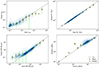 |
Fig. A.1. Results of our CIGALE mock analysis: Bayesian output parameters in relation to the known input parameters, using 100 SEDs for each galaxy that were randomly disturbed in flux. The blue shaded areas show the density of individual values in the plot. Green points and error bars show the mean and standard deviation in bins of input parameters. Orange points and error bars show the median and the 16th and 84th percentiles in the same bins. The dashed line represents a one-to-one ratio. |
Appendix B: Weight outliers
In our sample of QGs, two galaxies stand out with significantly higher stacking weights (i.e. better observed sensitivity). Although these galaxies are not individually detected (like all other galaxies in our sample) they would strongly dominate the stacked signals of the respective redshift bins that contain them. In Fig. B.1 we show the dust mass fraction for all QGs in our sample, which was inferred by performing aperture photometry on the ALMA images. The upper limits derived from stacking are generally lower than those inferred from individual galaxies, as is expected due to the improved depth of the stacks. The two high-weight galaxies fall in the z = 0.5 − 1 and z = 1 − 1.5 bins. In the z = 0.5 − 1 bin, the high-weight galaxy falls on the lower edge of the fdust distribution. Including this galaxy would have skewed the stack towards it, but the upper limit on fdust inferred from the stack would not have been significantly different. However, in the z = 1 − 1.5 bin, the single high-weight galaxy yields an individual dust mass limit that is a factor of ∼3 lower than that of the stack, and a factor of ∼10 lower than that of the next lowest individual galaxy. This one yields such a low dust mass fraction since it is undetected in a deep ALMA project (ASPECS-LP; González-López et al. 2019, 2020) and very massive (log(M*/M⊙)∼11.7). Including this galaxy in the stack would have yielded an fdust upper limit almost identical to that of this individual galaxy. While this QG is very constraining and therefore individually interesting, it is also not representative of the sample and, hence, needs to be excluded.
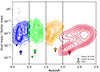 |
Fig. B.1. Dust mass fraction inferred for all individual QGs in our sample for different redshift bins. All QGs are individually undetected; therefore, triangles show the inferred 3 σ upper limits. The two high-weight galaxies are indicated by the large solid triangles and have redshifts of z ∼ 0.6 and z ∼ 1.1, respectively. Circles show the upper limits of the stacks in each bin as shown in Fig. 4 (i.e. without the high-weight sources). The coloured contours represent the number density distribution within each redshift bin. |
Appendix C: Influence of 24 μm-detected QGs
To investigate whether QGs that were individually detected in the Spitzer/MIPS 24 μm band have significantly different dust masses compared to those with undetected 24 μm fluxes, we split the stacks accordingly (Fig. C.1). We find no significant difference. Because the MIPS-detected galaxies constitute only ∼16% of the total sample, their stack upper limits on the dust mass fraction are statistically higher than those of the remaining sample. Their limits for the intermediate-redshift bins extend into the MS regime, but it remains unclear whether these MIPS-bright galaxies truly differ from the average QG population, as these measurements remain upper limits.
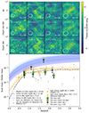 |
Fig. C.1. Same as Fig. 4 but now also showing stacking results for split samples, dividing galaxies with individual detections (dark green stars) from those with no detections (light green crosses) at 24 μm. |
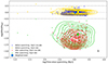 |
Fig. C.2. Location with respect to the Schreiber et al. (2015) MS as a function of the time since quenching for our full QG sample. Green (red) dots mark the locations of galaxies detected (undetected) in the 24 μm band after quenching, and yellow (blue) dots show the location of the same galaxies before quenching. The large symbols show the weighted mean of each group. The cross in the bottom-right corner denotes the error on the weighted mean. The coloured lines show the density distribution of each group. |
We further investigated the groups of 24 μm-detected and undetected QGs using the galaxy parameters yielded by CIGALE (Sect. 3.1). Figure C.2 shows ΔMSbefore quenching and ΔMSobs as a function of the time since quenching for 24 μm-detected and -undetected QGs in our sample. Before quenching, we find no difference between the two groups with respect to position within the MS. At the time of observation, the distribution of 24 μm-detected QGs extends to somewhat higher values of ΔMS than for 24 μm-undetected QGs, but still remains well below the MS. We find no significant difference between the weighted means of the two groups. The mean quenching times agree within 0.1 dex, close to 1 Gyr. The mean SFR of the 24 μm-detected QGs is ∼50% (i.e. ∼0.2 dex) higher than that of the 24 μm-undetected QGs. This tentatively hints that these QGs might be quenched less efficiently compared to the rest of the population, retaining potentially a slightly larger gas and dust reservoir. There is, however, no indication that these objects could be mis-identified SFGs contaminating our sample.
Appendix D: Rest-frame wavelengths
In Fig. D.1 we show the distribution of the rest-frame wavelengths in the stacks of Fig. 4, with vertical lines indicating the lower wavelength limit of the Rayleigh-Jeans spectral range, that is,  , for dust temperatures of 21 K and 17 K. Our stacks are clearly dominated by the Rayleigh-Jeans regime in redshift bins from 0.5 to 2, which contain the highest number of galaxies. Therefore, our wavelength rescaling of luminosities (see Sect. 3.2) is equivalent to a power-law rescaling (with an assumed dust emissivity index of β = 1.8; Magdis et al. 2021) and thus largely independent of the exact dust temperature, even when assuming low, yet reasonable temperatures of 17 K (Cochrane et al. 2022). In the redshift range > 2, the dominant part of the rest-frame wavelengths lie still within the Rayleigh-Jeans limit at 21 K, but move out for lower dust temperatures. Therefore, this particular bin is more sensitive to the chosen SED template and dust temperature. Naturally, a significant deviation of β, Δβ, from the assumed value of 1.8 could introduce an error into our rescaling. Accounting for this effect, we found that for our four redshift bins it would translate into uncertainties that would range from ∼1% to ∼7% for Δβ = 0.1 (i.e. a conservative dust emissivity dispersion measurement; e.g. Planck Collaboration XXV 2011), and from ∼10% to ∼50% for Δβ = 0.6 (i.e. a pessimistic dust emissivity dispersion measurement; e.g. Bendo et al. 2025).
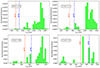 |
Fig. D.1. Normalised distribution of rest-frame wavelengths used to compute |


Appendix E: Acknowledgements
We would like to thank the anonymous referee for their comments that helped to improve the paper. SA and FB gratefully acknowledge the Collaborative Research Center 1601 (SFB 1601 sub-project C2) funded by the Deutsche Forschungsgemeinschaft (DFG, German Research Foundation) – 500700252. LC acknowledges support from the French government under the France 2030 investment plan, as part of the Initiative d’Excellence d’Aix-Marseille Université – A*MIDEX AMX-22-RE-AB-101. This paper makes use of the following ALMA data: ADS/JAO.ALMA#2015.1.00055.S, ADS/JAO.ALMA#2015.1.00098.S, ADS/JAO.ALMA#2015.1.00137.S, ADS/JAO.ALMA#2015.1.00207.S, ADS/JAO.ALMA#2015.1.00228.S, ADS/JAO.ALMA#2015.1.00260.S, ADS/JAO.ALMA#2015.1.00379.S, ADS/JAO.ALMA#2015.1.00543.S, ADS/JAO.ALMA#2015.1.00853.S, ADS/JAO.ALMA#2015.1.00861.S, ADS/JAO.ALMA#2015.1.00870.S, ADS/JAO.ALMA#2015.1.00948.S, ADS/JAO.ALMA#2015.1.01074.S, ADS/JAO.ALMA#2015.1.01205.S, ADS/JAO.ALMA#2015.1.01379.S, ADS/JAO.ALMA#2015.1.01447.S, ADS/JAO.ALMA#2015.1.01590.S, ADS/JAO.ALMA#2016.1.00171.S, ADS/JAO.ALMA#2016.1.00279.S, ADS/JAO.ALMA#2016.1.00324.L, ADS/JAO.ALMA#2016.1.00463.S, ADS/JAO.ALMA#2016.1.00564.S, ADS/JAO.ALMA#2016.1.00646.S, ADS/JAO.ALMA#2016.1.00790.S, ADS/JAO.ALMA#2016.1.00798.S, ADS/JAO.ALMA#2016.1.00804.S, ADS/JAO.ALMA#2016.1.00932.S, ADS/JAO.ALMA#2016.1.00967.S, ADS/JAO.ALMA#2016.1.00990.S, ADS/JAO.ALMA#2016.1.01001.S, ADS/JAO.ALMA#2016.1.01012.S, ADS/JAO.ALMA#2016.1.01040.S, ADS/JAO.ALMA#2016.1.01079.S, ADS/JAO.ALMA#2016.1.01155.S, ADS/JAO.ALMA#2016.1.01208.S, ADS/JAO.ALMA#2016.1.01355.S, ADS/JAO.ALMA#2016.1.01426.S, ADS/JAO.ALMA#2016.1.01454.S, ADS/JAO.ALMA#2016.1.01546.S, ADS/JAO.ALMA#2016.1.01604.S, ADS/JAO.ALMA#2017.1.00046.S, ADS/JAO.ALMA#2017.1.00138.S, ADS/JAO.ALMA#2017.1.00300.S, ADS/JAO.ALMA#2017.1.00326.S, ADS/JAO.ALMA#2017.1.00373.S, ADS/JAO.ALMA#2017.1.00428.L, ADS/JAO.ALMA#2017.1.00755.S, ADS/JAO.ALMA#2017.1.00893.S, ADS/JAO.ALMA#2017.1.01027.S, ADS/JAO.ALMA#2017.1.01099.S, ADS/JAO.ALMA#2017.1.01163.S, ADS/JAO.ALMA#2017.1.01176.S, ADS/JAO.ALMA#2017.1.01217.S, ADS/JAO.ALMA#2017.1.01359.S, ADS/JAO.ALMA#2017.1.01512.S, ADS/JAO.ALMA#2017.1.01618.S, ADS/JAO.ALMA#2017.1.01677.S, ADS/JAO.ALMA#2017.1.01713.S, ADS/JAO.ALMA#2017.A.00032.S, ADS/JAO.ALMA#2017.A.00034.S, ADS/JAO.ALMA#2018.1.00164.S, ADS/JAO.ALMA#2018.1.00231.S, ADS/JAO.ALMA#2018.1.00251.S, ADS/JAO.ALMA#2018.1.00329.S, ADS/JAO.ALMA#2018.1.00478.S, ADS/JAO.ALMA#2018.1.00543.S, ADS/JAO.ALMA#2018.1.00681.S, ADS/JAO.ALMA#2018.1.00874.S, ADS/JAO.ALMA#2018.1.00938.S, ADS/JAO.ALMA#2018.1.01044.S, ADS/JAO.ALMA#2018.1.01079.S, ADS/JAO.ALMA#2018.1.01128.S, ADS/JAO.ALMA#2018.1.01136.S, ADS/JAO.ALMA#2018.1.01225.S, ADS/JAO.ALMA#2018.1.01594.S, ADS/JAO.ALMA#2018.1.01739.S, ADS/JAO.ALMA#2018.1.01824.S, ADS/JAO.ALMA#2018.1.01841.S, ADS/JAO.ALMA#2018.1.01852.S, ADS/JAO.ALMA#2018.1.01871.S, ADS/JAO.ALMA#2019.1.00102.S, ADS/JAO.ALMA#2019.1.00459.S, ADS/JAO.ALMA#2019.1.00477.S, ADS/JAO.ALMA#2019.1.00652.S, ADS/JAO.ALMA#2019.1.00678.S, ADS/JAO.ALMA#2019.1.00702.S, ADS/JAO.ALMA#2019.1.00909.S, ADS/JAO.ALMA#2019.1.01127.S, ADS/JAO.ALMA#2019.1.01142.S, ADS/JAO.ALMA#2019.1.01201.S, ADS/JAO.ALMA#2019.1.01286.S, ADS/JAO.ALMA#2019.1.01528.S, ADS/JAO.ALMA#2019.1.01537.S, ADS/JAO.ALMA#2019.1.01600.S, ADS/JAO.ALMA#2019.1.01615.S, ADS/JAO.ALMA#2019.1.01634.L, ADS/JAO.ALMA#2019.1.01722.S, ADS/JAO.ALMA#2019.2.00118.S. ALMA is a partnership of ESO (representing its member states), NSF (USA) and NINS (Japan), together with NRC (Canada), NSTC and ASIAA (Taiwan), and KASI (Republic of Korea), in cooperation with the Republic of Chile. The Joint ALMA Observatory is operated by ESO, AUI/NRAO and NAOJ.
All Tables
Input parameters of the CIGALE module used for SED and SFH fitting of our QG sample.
All Figures
|
Fig. 1. Flow diagram of the selection of a robust QG sample. Blue panels denote general selections, orange panels the selection of QGs, red panels further cleaning steps, and green panels the number of QGs after every step. |
| In the text | |
|
Fig. 2. Normalised distribution of CIGALE-inferred Bayesian parameters of the parent sample of 4583 QGs and the 460 QGs in our A3COSMOS/A3GOODSS sample: SFR fraction (rSFR), stellar mass (M*), time since quenching (tq), and (ΔMS) before quenching and at the time of observation. We note that, due to the re-estimation of M* with CIGALE, a small number of galaxies fall slightly below the initial selection threshold of log(M*/M⊙) = 10.8. |
| In the text | |
|
Fig. 3. Characterisation of our sample of A3COSMOS/A3GOODSS QGs and the parent sample. Top panel: Time since quenching as a function of the observed redshift. The median error is shown on the right. Solid black lines indicate the locus of galaxies that quenched at the same time, from zq = 0.5 to 5 in steps of 0.5. The orange density map shows the distribution of the parent sample galaxies. The grey shaded areas in the background and dashed grey lines indicate the bins of quenching redshift and time since quenching used in Sect. 4.3. Middle panel: Distribution of quenching redshift (zq). Bottom panel: Fraction of recently quenched galaxies (tq ≤ 500 Myr). The points and horizontal error bars denote the median redshift and the 16th and 84th percentiles of all galaxies in each bin, respectively. The black line shows the fraction of recently quenched massive early-type galaxies as a function of redshift from Gobat et al. (2020). The dotted blue line and shaded area show our toy model based on the stellar mass functions of Davidzon et al. (2017). |
| In the text | |
|
Fig. 4. Results of our stacking of four different redshift bins: zobs = 0.5 − 1, 1 − 1.5, 1.5 − 2, and 2 − 3. Top panel: Cutouts of the map centre. We show the profile of the synthesised beam as a dashed white shape in the bottom left, and the number of individual galaxies stacked in the bottom right. The dashed red circle in the centre shows the aperture used to measure the source emission. The colour scaling is set to reflect the signal-to-noise ratio of each pixel. Bottom panel: Dust-to-stellar mass ratio (fdust) of our stacks (green diamonds) at the weighted mean redshift of each stack in comparison to the fdust measurements of massive QGs from the literature; grey symbols show individual measurements from dust (grey hexagons) and CO (grey squares), yellow symbols the results from stacking studies, and the dashed yellow and dash-dotted black lines the predictions from data fitting. The empty diamonds show our upper limits when assuming a lower dust temperature of 17 K. The dashed blue lines and shaded regions show the fdust evolution of massive MS galaxies from Liu et al. (2019b) and Wang et al. (2022). |
| In the text | |
|
Fig. 5. Dust mass at the time of observation divided by the dust mass of MS galaxies at the time of quenching as a function of time since quenching for three different bins of quenching redshift (green filled symbols). The empty symbols show the upper limits when assuming a lower dust temperature of 17 K. The yellow, orange-hatched, and red-chequered regions show the dust removal timescales from Michałowski et al. (2019, τ = 2.5 ± 0.4 Gyr), Leśniewska et al. (2023, τ = 2.26 ± 0.18 Gyr), and Nadolny et al. (2024, τ = 2.28 ± 0.1 Gyr), for three different fractional initial gas fractions (f0, gas). The empty purple symbol marks the f0, gas from the fit of Gobat et al. (2020). Light blue and dark blue symbols show dust mass evolution with time since quenching from Donevski et al. (2023) for spiral and elliptical QGs at z < 0.7, respectively, where we assume a 30% error on the dust mass, and the horizontal error bars denote the bin size of Donevski et al. (2023). |
| In the text | |
|
Fig. A.1. Results of our CIGALE mock analysis: Bayesian output parameters in relation to the known input parameters, using 100 SEDs for each galaxy that were randomly disturbed in flux. The blue shaded areas show the density of individual values in the plot. Green points and error bars show the mean and standard deviation in bins of input parameters. Orange points and error bars show the median and the 16th and 84th percentiles in the same bins. The dashed line represents a one-to-one ratio. |
| In the text | |
|
Fig. B.1. Dust mass fraction inferred for all individual QGs in our sample for different redshift bins. All QGs are individually undetected; therefore, triangles show the inferred 3 σ upper limits. The two high-weight galaxies are indicated by the large solid triangles and have redshifts of z ∼ 0.6 and z ∼ 1.1, respectively. Circles show the upper limits of the stacks in each bin as shown in Fig. 4 (i.e. without the high-weight sources). The coloured contours represent the number density distribution within each redshift bin. |
| In the text | |
|
Fig. C.1. Same as Fig. 4 but now also showing stacking results for split samples, dividing galaxies with individual detections (dark green stars) from those with no detections (light green crosses) at 24 μm. |
| In the text | |
|
Fig. C.2. Location with respect to the Schreiber et al. (2015) MS as a function of the time since quenching for our full QG sample. Green (red) dots mark the locations of galaxies detected (undetected) in the 24 μm band after quenching, and yellow (blue) dots show the location of the same galaxies before quenching. The large symbols show the weighted mean of each group. The cross in the bottom-right corner denotes the error on the weighted mean. The coloured lines show the density distribution of each group. |
| In the text | |
|
Fig. D.1. Normalised distribution of rest-frame wavelengths used to compute |
| In the text | |
Current usage metrics show cumulative count of Article Views (full-text article views including HTML views, PDF and ePub downloads, according to the available data) and Abstracts Views on Vision4Press platform.
Data correspond to usage on the plateform after 2015. The current usage metrics is available 48-96 hours after online publication and is updated daily on week days.
Initial download of the metrics may take a while.