| Issue |
A&A
Volume 702, October 2025
|
|
|---|---|---|
| Article Number | A207 | |
| Number of page(s) | 18 | |
| Section | Cosmology (including clusters of galaxies) | |
| DOI | https://doi.org/10.1051/0004-6361/202554474 | |
| Published online | 24 October 2025 | |
A roadmap to cosmological parameter analysis with third-order shear statistics
IV. Analytic cross-covariance between second- and third-order aperture masses
1
University of Bonn, Argelander-Institut für Astronomie, Auf dem Hügel 71, 53121 Bonn, Germany
2
School of Mathematics, Statistics and Physics, Newcastle University, Newcastle upon Tyne NE1 7RU, UK
3
Universität Innsbruck, Institut für Astro- und Teilchenphysik, Technikerstr. 25/8, 6020 Innsbruck, Austria
4
Waterloo Centre for Astrophysics, University of Waterloo, Waterloo, Ontario N2L 3G1, Canada
5
Department of Physics and Astronomy, University of Waterloo, Waterloo, Ontario N2L 3G1, Canada
6
Department of Astronomy and Astrophysics, University of California, Santa Cruz, 1156 High Street, Santa Cruz, CA 95064, USA
⋆ Corresponding author: This email address is being protected from spambots. You need JavaScript enabled to view it.
Received:
11
March
2025
Accepted:
25
August
2025
Abstract
Context. Weak gravitational lensing is a powerful probe of cosmology, with second-order shear statistics commonly used to constrain parameters such as the matter density Ωm and the clustering amplitude S8. However, degeneracies between parameters persist and can be broken by including higher-order statistics, such as the third-order aperture mass. To jointly analyse second- and third-order statistics, an accurate model of their cross-covariance is essential.
Aims. This work derives and validates a non-tomographic analytical model for the cross-covariance between second- and third-order aperture mass statistics. Analytical models are computationally efficient and enable cosmological parameter inference across a range of models, in contrast to numerical covariances derived from simulations or resampling methods, which are either costly or biased.
Methods. We derived the cross-covariance from real-space estimators of the aperture mass. Substituting the Halofit power spectrum, BiHalofit bispectrum, and a halo-model-based tetraspectrum, the model was validated against numerical covariances from the N-body Scinet LIghtCone Simulations (SLICS) using both shear catalogues and convergence maps. We performed a Markov chain Monte Carlo parameter analysis using both analytical and numerical covariances for several filter scale combinations.
Results. The cross-covariance separates into three terms governed by the power spectrum, bispectrum, and tetraspectrum, with the latter dominating. While the analytical model qualitatively reproduces simulation results, differences arise due to modelling approximations and numerical evaluation issues. The analytical contours are systematically tighter, with a combined figure of merit that is 72% that of the numerical case, increasing to 80% when small-scale information is excluded. These differences largely stem from an underprediction of the second-order covariance.
Conclusions. This work completes the analytical covariance framework for second- and third-order aperture mass statistics, enabling joint parameter inference without the need for large simulation suites. While further refinement is needed to improve quantitative accuracy, the model represents a key step towards simulation-independent cosmic shear analyses.
Key words: gravitational lensing: weak / methods: analytical / methods: statistical / cosmological parameters / large-scale structure of Universe
© The Authors 2025
 Open Access article, published by EDP Sciences, under the terms of the Creative Commons Attribution License (https://creativecommons.org/licenses/by/4.0), which permits unrestricted use, distribution, and reproduction in any medium, provided the original work is properly cited.
This article is published in open access under the Subscribe to Open model. This email address is being protected from spambots. You need JavaScript enabled to view it. to support open access publication.
1. Introduction
The Lambda cold dark matter (ΛCDM) model is the prevailing framework for understanding the evolution of the Universe, from the post-inflationary epoch to the development of the large-scale structure (LSS) observed today. It is characterised by six key parameters that must be empirically determined. Observational efforts to constrain these parameters fall into two broad categories: those that examine the early Universe through measurements of the cosmic microwave background (CMB), such as those provided by Planck (Planck Collaboration VI 2020), and those that probe the late-time Universe, notably via the LSS.
A longstanding area of interest in recent years has been the apparent tension between CMB-based and LSS-based determinations of the clustering amplitude parameter  , where σ8 quantifies the normalisation of the matter power spectrum and Ωm denotes the total matter density. Several LSS surveys have reported lower values of S8 compared to those inferred from the CMB, with tensions reaching 2 − 3σ significance (Di Valentino et al. 2021; Joudaki et al. 2020; Asgari et al. 2021). However, recent results from the KiDS-Legacy analysis (Wright et al. 2025) have shown that this tension can be resolved through a more robust statistical treatment of the data, suggesting that the discrepancy does not require new physics, but rather a refined methodological framework.
Nevertheless, the potential of weak gravitational lensing as a tool for probing cosmology remains undiminished. Through the measurement of background galaxy distortions induced by the intervening matter distribution, weak lensing offers a direct and unbiased probe of the total matter content, encompassing both baryonic and dark components, without assumptions about galaxy bias. This makes it uniquely suited for constraining key cosmological parameters such as Ωm and S8 (σ8).
In the past decade, weak lensing analyses have primarily employed second-order statistics, such as the two-point shear correlation function, which have substantially improved parameter constraints (Hildebrandt et al. 2017; DES Collaboration 2022; Heymans et al. 2021; Dalal et al. 2023). However, second-order measures alone are limited in their ability to fully characterise the matter distribution, particularly at late times. The Gaussian approximation valid in the early Universe breaks down due to non-linear structure formation, which induces non-Gaussian features such as high-density peaks corresponding to galaxy clusters. These complexities are not captured by second-order statistics alone.
Moreover, degeneracies, especially between Ωm and σ8, remain a significant challenge when relying solely on two-point statistics (Takada & Jain 2004; Kilbinger & Schneider 2005; Euclid Collaboration: Ajani et al. 2023). To break these degeneracies and access the richer information encoded in the LSS, higher-order statistics and non-Gaussian probes have become an increasingly active area of development. These methods hold the potential not only to tighten parameter constraints, but also to offer a more complete statistical description of the cosmic matter distribution.
In the following, we focus on third-order statistics, which provide a measure of the skewness of the matter distribution. Since second- and third-order statistics have different dependences on Ωm and S8 (Takada & Jain 2004; Kilbinger & Schneider 2005; Kayo et al. 2013; Pyne & Joachimi 2021), combining them in a joint parameter analysis helps to break degeneracies, as demonstrated by Heydenreich et al. (2023). Various higher-order statistics have been introduced to address the limitations of second-order statistics in weak gravitational lensing. Examples include the shear three-point correlation function (Schneider & Lombardi 2003; Schneider et al. 2005), peak-count statistics (Martinet et al. 2018; Harnois-Déraps et al. 2021), persistent homology (Heydenreich et al. 2021), and density split statistics (Gruen et al. 2018; Burger et al. 2022). For our analysis, we adopted second- and third-order aperture mass statistics, ⟨ℳap2⟩ and ⟨ℳap3⟩, due to several advantages. Firstly, they are scalars, which effectively compress data and simplify handling (Heydenreich et al. 2023). Secondly, they are unaffected by the mass-sheet degeneracy, a transformation that adds a constant 1 − λ to the dimensionless surface mass density, while linearly scaling it by λ, leaving lensing observables unchanged (Falco et al. 1985; Schneider & Seitz 1995). Thirdly, they naturally decompose E- and B-modes, where B-modes should not be present in gravitational lensing to leading order, providing a valuable check for systematic errors. Lastly, they can be analytically modelled in a comparatively simple manner.
This paper is part of a series that presents a comprehensive approach to cosmological parameter estimation using third-order shear statistics. The series begins with an in-depth analysis of the analytical model for ⟨ℳap3⟩ (Heydenreich et al. 2023). The second paper derives the analytical auto-covariance for ⟨ℳap3⟩ (Linke et al. 2023, L+23 hereafter). The third paper Porth et al. (2024) introduces an efficient method for computing aperture mass statistics by measuring the shear three-point correlation function (3PCF). Finally, the last paper (Burger et al. 2024) presents the first numerical cosmological parameter analysis of the fourth data release of the Kilo-Degree Survey (KiDS-1000), incorporating second- and third-order shear statistics, intrinsic alignments, and the effects of baryonic feedback. The current paper establishes the foundation for an analytical joint analysis of ⟨ℳap2⟩ and ⟨ℳap3⟩ by deriving the final missing component: the analytical cross-covariance. Once derived, we validated the cross-covariance through a joint parameter analysis on simulated data. To achieve this, we used the analytical third-order auto-covariance from L+23 and the analytical second-order auto-covariance computed in Linke et al. (2024). By combining these covariances with the cross-covariance, we were able to construct posterior distributions using Markov chain Monte Carlo (MCMC) sampling.
Using an analytical covariance instead of a numerical one provides several advantages. A numerical covariance can be obtained either from simulations or directly from observational data. In the case of simulations, the number of realisations required must significantly exceed the number of components in the data vector, making the approach computationally expensive. Running these simulations and computing the covariance is particularly demanding, as data vectors are often large. In contrast, an analytical model significantly reduces computational cost while maintaining accuracy. Alternatively, the covariance matrix can be estimated using jackknife resampling or bootstrapping. These methods divide the data field into multiple patches that are small enough to ensure there are more patches than data vector components, and compute the sample covariance over these patches. However, this approach has limitations. It neglects correlations on scales larger than the patch size and assumes that the patches are mutually independent, which is not strictly true since adjacent patches share boundaries. As a result, this method introduces a bias in the covariance estimate, whereas an analytical covariance remains unaffected. Moreover, an analytical approach enables a straightforward evaluation of the covariance under different cosmological models. This is crucial for parameter inference and forecasting, as observational data by definition only samples a single cosmology, and generating large suites of simulations for multiple cosmologies would be prohibitively expensive.
The paper is organised as follows. Section 2 provides a concise review of aperture mass statistics. Section 3 introduces real-space estimators for aperture mass statistics and derives the analytical cross-covariance from these estimators. Additionally, we present a numerical method for validating the analytical results. Section 4 compares the analytical and numerical cross-covariances, where the analytical model is constructed by adapting the publicly available third-order modelling code threepoint1. Section 5 outlines the joint cosmological parameter estimation and its validation against numerical contours. Finally, Sect. 6 discusses our findings and presents concluding remarks.
2. Theoretical background
This section briefly overviews the key quantities of weak gravitational lensing and aperture masses. A more detailed discussion can be found in Schneider (1996), Bartelmann & Schneider (2001), Hoekstra & Jain (2008) or Bartelmann (2010). This paper assumes a flat universe, such that the comoving angular-diameter distance equals the comoving radial distance fK(χ) = χ. Furthermore, we use the flat-sky approximation. The matter density contrast is  , where
  is the matter density at angular position ϑ and comoving distance χ on the backward light cone, and
  is the average density at χ. Defining the Fourier transform of variables with a tilde, the polyspectra of the density contrast 𝒫n(3d) are defined by
 (1)
(1)
where ⟨…⟩c are cumulants or connected correlation functions, and δD is a Dirac delta function.
2.1. The convergence
The convergence, or the dimensionless surface mass density, can be calculated from δ by a weighted line-of-sight integration
 (2)
(2)
the Hubble constant H0, the probability distribution of source galaxies in comoving distance p(χ) dχ, the speed of light c, and the scale factor a(χ), normalised to unity today. The nth-order polyspectra 𝒫n of the convergence are defined by
 (3)
(3)
Here and in the following, integrals without explicit boundaries are integrals over ℝ2. Particularly, the power spectrum P, the bispectrum B, and the tetraspectrum P5 are the convergence polyspectra important for our present discussion and are defined as
 (4)
(4)
where we made use of the homogeneity and isotropy of the Universe. Under the Limber approximation, they are related to the polyspectra of δ (𝒫n(3d)) by a weighted integration along the line of sight (Limber 1954; Kaiser & Jaffe 1997; Kayo et al. 2013):
 (5)
(5)
The convergence defined in Eq. (2) and its nth-order connected correlation function (Eq. (3)) will be used to calculate the aperture mass in the following subsection, from which our statistics are derived. If shape noise from the intrinsic ellipticity of galaxies, ϵi, is present, it must be accounted for by adding σϵi2/(2N) to the power spectrum P(ℓ), where σϵi is the two-component intrinsic ellipticity dispersion and N is the galaxy number density. A proof of this correction can be found in Appendix B of L+23. Since shape noise is Gaussian, it does not affect the bispectrum or tetraspectrum.
2.2. Definition of the aperture mass
The aperture mass ℳap can be calculated by either a weighted two-dimensional integration over the convergence or the tangential shear γt. It was first introduced in Schneider (1996), and can be defined by either
 (6)
(6)
where ϕ is the aperture centre coordinate, θ the filter radius, and Uθ and Qθ are radially symmetric filter functions. Uθ is compensated, obeying the relation
 (7)
(7)
For our purpose, we use the exponential filter function proposed in Crittenden et al. (2002),
 (8)
(8)
The Fourier transform of Uθ is
 (9)
(9)
The second- and third-order aperture mass statistics are essential for our present discussion and are defined, respectively, by
 (10)
(10)
where ⟨…⟩ denotes the spatial average over ϕ. We note that since ⟨ℳap⟩ = 0, as the expectation value of the density contrast δ is by definition zero, the second- and third-order cumulants of the aperture mass are equal to the spatial averages: ⟨ℳap3⟩c = ⟨ℳap3⟩ and ⟨ℳap2⟩c = ⟨ℳap2⟩. Inserting the definition of the aperture mass calculated from the convergence (Eq. (6)) into the Eq. (10), using that the spatial averages are equal to the cumulants and substituting the cumulants of the convergence with the polyspectra as defined in Eq. (3), one finds
 (11)
(11)
for the second-order aperture mass statistics, where going from the first to the second line, we performed the Fourier transformation on the Uθ filters. In the last step, we integrated the Dirac delta function. It is important to note that taking equal aperture radii for the second-order aperture mass statistics (i.e., θ1 = θ2) captures all the information in this order. With the chosen  filter (Eq. (9)), the dispersion at two distinct aperture radii can be expressed as a dispersion at an average aperture radius (Schneider et al. 2005)
 (12)
(12)
Therefore, using equal aperture radii in the dispersion preserves all relevant information, and it is sufficient to evaluate ⟨ℳap2⟩(θ):=⟨ℳap2⟩(θ, θ) with a single aperture radius as input. Equivalently, for the third-order
 (13)
(13)
The simplification to equal aperture radii used above is not applicable to the third-order statistics. This can be observed from Eq. (9), which sharply peaks around  . For ⟨ℳap3⟩, if one were to take θ1 = θ2 = θ3 in Eq. (13), only equilateral configurations of the bispectrum with
  would be probed (Schneider et al. 2005). However, the non-equilateral aperture radii configurations depend on different bispectrum configurations and provide additional information in this order. Therefore, distinct aperture radii should be allowed for third-order statistics.
3. Derivation of the analytical cross-covariance
In a real survey or simulation, convolving with the weight function Uθ over an infinite area is not feasible. Therefore, following L+23, we define a real-space estimator of the aperture mass as
 (14)
(14)
where A′ represents the finite survey area. By spatially averaging products of this real-space estimator over the aperture centre ϕ, we estimate the second- and third-order aperture mass statistics. However, since we are working with a finite survey area, this spatial average is itself an approximation. Moreover, the averaging region must be smaller than the full survey area, as the aperture mass involves integrating over a region surrounding the aperture centre. Placing aperture centres too close to the survey boundary would introduce biases due to boundary effects. To mitigate these effects, we estimate the second- and third-order aperture mass statistics by averaging over an area A, which is entirely contained within the survey region A′ as illustrated in Fig. 1. The area A is chosen such that 99.9% of the effective support of Qθ is within A′ when the aperture centre ϕ is placed on the boundary of A and the largest aperture radius θmax is used. This condition is satisfied when the boundary of A is positioned 4 θmax inside the boundary of A′ (Heydenreich et al. 2023). The field boundary of A is determined using Qθ rather than Uθ because Uθ is a compensated filter function, meaning its support is not well-defined in the same way. Given this set-up, the integrals over the finite survey area A′ can be approximated as integrals over the entire real space ℝ2, since the convolution with Uθ contributes negligibly outside of A′. The real-space statistics of the aperture mass are thus given by
![Mathematical equation: $$ \begin{aligned} \hat{\mathcal{M} }_{\mathrm{ap}}^{2}(\theta ) = \frac{1}{A} \int _A \mathrm{d}^2\phi \; \left[ \prod _{i = 1}^2 \int \mathrm{d}^2\vartheta _i \; U_{\theta }\left(|\phi -\vartheta _i|\right) \, \kappa (\vartheta _i)\right] \;\;\text{ and}\;\; \hat{\mathcal{M} }_{\mathrm{ap}}^{3}(\theta _1,\theta _2,\theta _3) = \frac{1}{A} \int _A \mathrm{d}^2\phi \; \left[ \prod _{i = 1}^3 \int \mathrm{d}^2\vartheta _i \; U_{\theta _i}\left(|\phi -\vartheta _i|\right) \, \kappa (\vartheta _i) \right] \;. \end{aligned} $$](/articles/aa/full_html/2025/10/aa54474-25/aa54474-25-eq22.gif) (15)
(15)
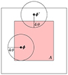 |
Fig. 1. Aperture centre placement in a data field (from L+23). Given a data field of area A′ (not necessarily a square field), apertures are only placed within a smaller field A, which lies well within A′. The boundary of A is chosen such that 99.9% of the effective support of Qθ lies within A (which corresponds to ∼4 θ) if the aperture centre lies on this boundary. To illustrate this, two aperture centres are depicted: ϕ is within A and ϕ″ is outside of A. It can be seen that the circle around ϕ″, illustrating the effective support of Qθ, extends beyond A′, thus introducing bias into the calculated aperture mass at this point. To exclude this effect, we only average the aperture centre over the red region A. |
The cross-covariance of the real-space estimators is then defined as
 (16)
(16)
Here and in the following, when a comma ‘,’ is used, the function is invariant under permutations of its arguments, whereas when a semi-colon ‘;’ is used, they are not invariant. The first term in Eq. (16) is given as
![Mathematical equation: $$ \begin{aligned} \Big \langle \hat{\mathcal{M} }_{\mathrm{ap}}^{3}\hat{\mathcal{M} }_{\mathrm{ap}}^{2}\Big \rangle (\theta _1,\theta _2,\theta _3;\theta _4) =&\; \frac{1}{A^2} \int _A \mathrm{d}^2\phi _1 \int _A \mathrm{d}^2\phi _2 \; \left[ \prod _{i = 1}^3 \int \mathrm{d}^2\vartheta _i \; U_{\theta _i}\left(|\phi _1-\vartheta _i|\right) \right] \left[ \prod _{j = 4}^5 \int \mathrm{d}^2\vartheta _j \; U_{\theta _4}\left(|\phi _2-\vartheta _j|\right)\right] \nonumber \\&\times \Big \langle \kappa (\vartheta _1)\kappa (\vartheta _2) \kappa (\vartheta _3) \kappa (\vartheta _4) \kappa (\vartheta _5)\Big \rangle \;. \end{aligned} $$](/articles/aa/full_html/2025/10/aa54474-25/aa54474-25-eq24.gif) (17)
(17)
Here, the fifth-order correlation function can be separated into cumulants,
![Mathematical equation: $$ \begin{aligned} \Big \langle \hat{\mathcal{M} }_{\mathrm{ap}}^{3}\hat{\mathcal{M} }_{\mathrm{ap}}^{2}\Big \rangle (\theta _1,\theta _2,\theta _3;\theta _4) =&\; \frac{1}{A^2} \int _A \mathrm{d}^2\phi _1 \int _A \mathrm{d}^2\phi _2 \; \left[ \prod _{i = 1}^3 \int \mathrm{d}^2\vartheta _i \; U_{\theta _i}\left(|\phi _1-\vartheta _i|\right)\right] \left[ \prod _{j = 4}^5 \int \mathrm{d}^2\vartheta _j \; U_{\theta _4}\left(|\phi _2-\vartheta _j|\right)\right] \nonumber \\&\times \Bigg \{ \Big \langle \kappa (\vartheta _1) \, \kappa (\vartheta _2) \, \kappa (\vartheta _3)\Big \rangle _{\rm c} \, \Big \langle \kappa (\vartheta _4) \, \kappa (\vartheta _5)\Big \rangle _{\rm c} \nonumber \\&+ \Big \langle \kappa (\vartheta _1) \, \kappa (\vartheta _4) \, \kappa (\vartheta _5)\Big \rangle _{\rm c} \, \Big \langle \kappa (\vartheta _2) \, \kappa (\vartheta _3)\Big \rangle _{\rm c} + \, 2\,\mathrm{Perm.\,of}\,(\theta _1,\theta _2,\theta _3) \\&+ 2\Big [\Big \langle \kappa (\vartheta _1) \, \kappa (\vartheta _2) \, \kappa (\vartheta _4)\Big \rangle _{\rm c} \, \Big \langle \kappa (\vartheta _3) \, \kappa (\vartheta _5)\Big \rangle _{\rm c} + \, 2\,\mathrm{Perm.\,of}\,(\theta _1,\theta _2,\theta _3) \Big ] \nonumber \\&+ \Big \langle \kappa (\vartheta _1) \, \kappa (\vartheta _2) \, \kappa (\vartheta _3) \, \kappa (\vartheta _4) \, \kappa (\vartheta _5)\Big \rangle _{\rm c}\Bigg \} \nonumber \\ =:&\; T_{\rm PB,1}(\theta _1,\theta _2,\theta _3;\theta _4)+T_{\rm PB,2}(\theta _1,\theta _2,\theta _3;\theta _4)+T_{\rm PB,3}(\theta _1,\theta _2,\theta _3;\theta _4) + T_{\rm P5}(\theta _1,\theta _2,\theta _3;\theta _4)\; , \nonumber \end{aligned} $$](/articles/aa/full_html/2025/10/aa54474-25/aa54474-25-eq25.gif) (18)
(18)
where we defined the T-expressions such that TPB, 1 corresponds to the term in the second line, TPB, 2 to the third, TPB, 3 to the fourth, and TP5 to the fifth. The permutations of TPB, 2 and TPB, 3 can be found in Table 1. The third term (TPB, 3) includes a factor of two because swapping  with
with  results in equivalent terms, as both are connected to θ4. Remember ⟨κ⟩ = 0 because the expectation value of the density contrast δ is zero; thus, the second- and third-order cumulants of the convergence are equal to the respective moments: ⟨κ3⟩c = ⟨κ3⟩ and ⟨κ2⟩c = ⟨κ2⟩ (but ⟨κ5⟩c ≠ ⟨κ5⟩). As a result, TPB, 1 cancels the second term on the r.h.s. of Eq. (16), observing it can be written as the expectation value of
  times the expectation value of
  , such that
Aperture scale radii permutations for TPB, 2 and TPB, 3.
 (19)
(19)
The second term TPB, 2 can be rewritten by substituting the definition for the convergence polyspectra (Eq. (3)) into Eq. (18), cancelling ℓ3 and ℓ5 by integrating over the Dirac delta functions and performing the Fourier transformations of the Uθ functions
![Mathematical equation: $$ \begin{aligned} T_{\rm PB,2}(\theta _1,\theta _2,\theta _3;\theta _4) = &\;\frac{1}{A^2} \int _A \mathrm{d}^2\phi _1 \int _A \mathrm{d}^2\phi _2 \; \left[\prod _{i = 1}^3 \int \mathrm{d}^2\vartheta _i \; U_{\theta _i}\left(|\phi _1-\vartheta _i|\right)\right] \left[\prod _{j = 4}^5 \int \mathrm{d}^2\vartheta _j \; U_{\theta _4}\left(|\phi _2-\vartheta _j|\right)\right]\prod _{k = 1}^5\int \frac{\mathrm{d}^2\ell _k}{(2\pi )^{6}} \nonumber \\&\times \delta _{\rm D}(\ell _2+\ell _3)\, \delta _{\rm D}(\ell _1+\ell _4+\ell _5)\, \mathcal{P} _3(\ell _1,\ell _4, \ell _5) \, \mathcal{P} _2(\ell _2,\ell _3)\, \mathrm{e}^{-\mathrm{i}\,(\ell _1\cdot \vartheta _1+\ell _2\cdot \vartheta _2+\ell _3\cdot \vartheta _3+\ell _4\cdot \vartheta _4+\ell _5\cdot \vartheta _5)} \nonumber \\&+ \, 2\,\mathrm{Perm.\,of}\,(\theta _1,\theta _2,\theta _3)\nonumber \\ =&\; \frac{1}{A^2} \int _A \mathrm{d}^2\phi _1 \int _A \mathrm{d}^2\phi _2 \; \left[\prod _{i = 1}^3 \int \mathrm{d}^2\vartheta _i \; U_{\theta _i}\left(|\phi _1-\vartheta _i|\right)\right] \left[ \prod _{j = 4}^5 \int \mathrm{d}^2\vartheta _j \; U_{\theta _4}\left(|\phi _2-\vartheta _j|\right)\right]\,\int \frac{\mathrm{d}^2\ell _1}{(2\pi )^2}\int \frac{\mathrm{d}^2\ell _2}{(2\pi )^2}\\&\times \int \frac{\mathrm{d}^2\ell _4}{(2\pi )^2}\,B(\ell _1,\ell _4)\, P(\ell _2)\, \mathrm{e}^{-\mathrm{i}\,(\ell _1\cdot (\vartheta _1-\vartheta _5)+\ell _2\cdot (\vartheta _2- \vartheta _3)+\ell _4\cdot (\vartheta _4- \vartheta _5))}+ \, 2\,\mathrm{Perm.\,of}\,(\theta _1,\theta _2,\theta _3) \nonumber \\ =&\;\frac{1}{A^2} \int _A \mathrm{d}^2\phi _1 \int _A \mathrm{d}^2\phi _2\; \int \frac{\mathrm{d}^2\ell _1}{(2\pi )^2}\int \frac{\mathrm{d}^2\ell _2}{(2\pi )^2} \int \frac{\mathrm{d}^2\ell _4}{(2\pi )^2} \; B(\ell _1,\ell _4)\, P(\ell _2) \nonumber \\&\times \tilde{u}(\ell _1 \theta _1) \, \tilde{u}(\ell _2 \theta _2) \, \tilde{u}(\ell _2 \theta _3) \, \tilde{u}(\ell _4 \theta _4) \, \tilde{u}(|\ell _1+\ell _4|\, \theta _4)\, \mathrm{e}^{-\mathrm{i}\,\ell _1\cdot (\phi _1-\phi _2)}+ \, 2\,\mathrm{Perm.\,of}\,(\theta _1,\theta _2,\theta _3)\;. \nonumber \end{aligned} $$](/articles/aa/full_html/2025/10/aa54474-25/aa54474-25-eq31.gif) (20)
(20)
Collecting all terms containing information on the survey area and geometry in the geometry factor  defined as (L+23)
 (21)
(21)
we find the final result
 (22)
(22)
By equivalent calculations, one finds
 (23)
(23)
and
 (24)
(24)
Equations ((22)–(24)) can subsequently be substituted into Eq. (19) to obtain the analytical covariance of the real-space estimator. Next, we investigate how these terms scale with the survey field size.
3.1. Large survey area approximation
This subsection illustrates how the cross-covariance terms behave as the field size increases, by taking the limit A → ∞ in the geometry factor (Eq. (21)). In this limit, one finds (L+23)
 (25)
(25)
Substituting and eliminating ℓ1 by integrating over the Dirac delta function, the large-field approximation of TPB, 2 becomes
 (26)
(26)
because  , as can be seen from Eq. (9). Thus, TPB, 2 arises solely from the limited size of the survey field and will therefore be referred to as a finite-field term.
For TPB, 3 and TP5, as given in Eqs. (23) and (24) respectively, the foregoing limiting procedure leads to
 (27)
(27)
and
 (28)
(28)
such that the cross-covariance in the large-field approximation simplifies to
 (29)
(29)
While TPB, 3 and TP5 scale approximately as 1/A, TPB, 2 exhibits a steeper decline with increasing field size.
Since the geometry term (Eq. (21)) is a rapidly oscillating function, its integration presents numerical challenges. Because our computational resources are largely sufficient for this task (albeit with some limitations; see Sect. 6.1), we retain the full expressions. However, in scenarios with limited computing power, or when computational efficiency is prioritised, large-field approximations may serve as useful alternatives.
A concluding remark on the derived cross-covariance and its large-field approximation is that to compute their values, we estimate P5 in TP5 using a halo decomposition (Appendix A). TP5 is then approximated by keeping the two dominant terms, the one-halo term and one of the two-halo terms:
 (30)
(30)
In the large-field approximation TP5, 2h∞ = 0, which means this is a finite field term, and thus we find TP5∞ ≈ TP5, 1h∞.
3.2. Aperture mass correlation functions
This section demonstrates that the covariance terms (Eqs. (22)–(24)) can alternatively be constructed with aperture mass correlation functions. These correlation functions can be numerically estimated from N-body simulations and therefore enable us to verify the individual components of our analytical cross-covariance.
The aperture mass correlation functions are defined as
![Mathematical equation: $$ \begin{aligned}&\mathcal{M} _{\rm ap}^{n,m}(\theta _1,\dots ,\theta _{m};\theta _{m+1},\dots ,\theta _n;\eta ):=\Big \langle \mathcal{M} _{\mathrm{ap}}(\phi ,\theta _1) \dots \mathcal{M} _{\mathrm{ap}}(\phi ,\theta _m)\,\mathcal{M} _{\mathrm{ap}}(\phi +\eta ,\theta _{m+1})\dots \mathcal{M} _{\mathrm{ap}}(\phi +\eta ,\theta _n)\Big \rangle \nonumber \\&=\left[ \prod _{i = 1}^m\int \mathrm{d}^2\vartheta _i \;U_{\theta _1}(\vartheta _1)\dots U_{\theta _m}(\vartheta _m)\right] \left[ \prod _{j=m+1}^n \int \mathrm{d}^2\vartheta _j \; U_{\theta _{m+1}}\left(\mid {\vartheta _{m+1}+\eta }\mid \right)\dots U_{\theta _{n}}\left(\mid {\vartheta _{n}+\eta }\mid \right)\right]\,\Big \langle \kappa (\vartheta _1)\dots \kappa (\vartheta _n)\Big \rangle \;, \end{aligned} $$](/articles/aa/full_html/2025/10/aa54474-25/aa54474-25-eq44.gif) (31)
(31)
where, without loss of generality, we set ϕ = 0 after the equality sign by shifting the origin. Substituting the correlation functions into Eq. (18), TPB, 2 is rewritten as
 (32)
(32)
By replacing the ϕ2 integral by an η = ϕ1−ϕ2 integral and integrating over d[2]ϕ1, we obtain  , where
  represents the probability that for a point ϕ1 within A, the point ϕ1 + η also lies within A. For a square survey area,
  is given in Appendix A.2 of Heydenreich et al. (2020). By expanding these algebraic steps, we find
 (33)
(33)
After generating the aperture mass correlation function maps from simulations, we azimuthally average them over the polar angle of η due to the statistical isotropy of the Universe. Defining the aperture mass correlations as a function of distance η by  (Eq. (31) cannot be used in this context, as it requires a vector-valued input η) and integrating
  over the polar angle of η, one finds
 (34)
(34)
where for a survey of square area, EA(η) is given in Appendix A.2 of Heydenreich et al. (2020)2 as
![Mathematical equation: $$ \begin{aligned} E_A(\eta ) = {\left\{ \begin{array}{ll} \frac{1}{A\pi }\left[A\pi -\left(4\sqrt{A}-\eta \right)\,\eta \right]\quad&\text{ for}\quad \eta \le \sqrt{A}\;,\\ \frac{2}{\pi }\left[2\sqrt{\frac{\eta ^2}{A}-1}-1-\frac{\eta ^2}{2A}-\arccos \left(\frac{\sqrt{A}}{\eta }\right)+\arcsin \left(\frac{\sqrt{A}}{\eta }\right)\right]\quad&\text{ for}\quad \sqrt{A}\le \eta \le \sqrt{2A}\;,\\ 0 \quad&\text{ for}\quad \sqrt{2A}\le \eta \;. \end{array}\right.} \end{aligned} $$](/articles/aa/full_html/2025/10/aa54474-25/aa54474-25-eq53.gif) (35)
(35)
Following the same procedure for TPB, 1 and TPB, 3 leads to
 (36)
(36)
 (37)
(37)
We note that because Eq. (18) is written in cumulants, TP5 cannot be simply connected to the fifth-order correlation function. Therefore, to calculate TP5 in terms of correlation functions, we subtract TPB, 1, TPB, 2, and TPB, 3 as defined above, such that
 (38)
(38)
4. Analytical model validation
With a model for the analytical cross-covariance of the second- and third-order aperture mass statistics in hand, it is important to test its consistency with N-body simulations.
4.1. Covariance estimation methods from simulations
A numerical cross-covariance can be obtained from simulations in two ways. The first and most straightforward method involves taking the unbiased sample covariance from multiple simulation realisations. For this approach, a significantly larger number of realisations (lines of sight) is required than the number of components in the data vector, and these realisations must be independent of one another. As discussed in Sect. 3, we need to exclude the boundaries of the fields by cutting off four times the largest aperture radius, θmax. After spatially averaging the second- and third-order aperture mass over its centre coordinate ϕ ( and
and  , respectively) for each realisation i, the sample covariance is computed using
![Mathematical equation: $$ \begin{aligned} C^{\mathrm{sim}}_{\hat{\mathcal{M} }_{\rm ap}^{3,2}} (\theta _1,\theta _2,\theta _3;\theta _4) = \frac{1}{N-1}\sum ^N_{i = 1} \left[ \hat{\mathcal{M} }_{\rm ap}^3(\theta _1,\theta _2,\theta _3) \right]_i \,\left[ \hat{\mathcal{M} }_{\rm ap}^2(\theta _4) \right]_i - \frac{1}{N(N-1)}\sum ^N_{i = 1} \left[ \hat{\mathcal{M} }_{\rm ap}^3(\theta _1,\theta _2,\theta _3) \right]_i \, \sum ^N_{j = 1} \left[ \hat{\mathcal{M} }_{\rm ap}^2(\theta _4) \right]_j\;, \end{aligned} $$](/articles/aa/full_html/2025/10/aa54474-25/aa54474-25-eq59.gif) (39)
(39)
where the sums are taken over the realisations, and N represents the number of realisations.
The second method involves using aperture mass correlation function maps, as outlined in Sect. 3.2. It is important to note that the same boundary exclusion must be applied for this method. The advantage of this approach is that it allows us to obtain the T-terms separately.
The sum of TPB, 2, TPB, 3, and TP5, computed from the aperture mass correlation function maps (Eqs. (34), (37), and (38)), reproduces the full sample covariance. We use the individually measured T-terms solely for comparison with their analytical counterparts. In analyses that rely on the full numerical covariance, such as the cosmological parameter estimations in Sect. 5, we adopt the sample covariance as our reference, as this allows us to estimate errors via bootstrapping.
4.2. Validation simulation – SLICS
We use the Scinet-LIghtCone Simulations (SLICS hereafter; Harnois-Déraps & van Waerbeke 2015; Harnois-Déraps et al. 2018) to validate the analytical model. These are dark matter only N-body simulations from which we use both shear catalogues and convergence maps. The SLICS are a suite of ray-tracing simulations which use 15363 particles placed in a 505 h−1 Mpc box. A flat ΛCDM cosmology is assumed, with normalised Hubble constant h = 0.69, the normalisation of the power spectrum σ8 = 0.83, the equation of state of dark matter w = −1, matter density parameter Ωm = 0.29, baryon density parameter Ωb = 0.047, and primordial power spectrum spectral index ns = 0.969. For the set of convergence maps, we use 715 independent lines of sight, all having an area of 10 × 10 deg2, placed on a 7745 × 7745 pixel grid. All maps have a redshift of z = 0.897, assume the flat-sky approximation, and do not contain shape noise. The aperture mass maps are calculated using the first equation in Eq. (6). The shear catalogue set contains 927 independent lines of sight, and has a galaxy number density
 (40)
(40)
where z0 = 0.637, β = 1.5, and the galaxy density is normalised to 30 arcmin−2, mimicking a density that is expected in the Euclid survey (Laureijs et al. 2011; Euclid Collaboration: Mellier et al. 2025). The galaxies have a maximum redshift of zmax = 3. Each realisation has again an area of 10 × 10 deg2. Every galaxy contains a shear, upon which an intrinsic ellipticity is added as shape noise. This is done by adding a random ellipticity to the shear from a Gaussian with a two-component ellipticity dispersion of σϵ2 = (0.37)2. The aperture mass is estimated by a weighted summation over the ellipticities of the galaxies
 (41)
(41)
where N is the total number of galaxies in the catalogue and ϵt, i is the sum of the tangential shear plus the tangential intrinsic ellipticity for the galaxy i. This is a discrete approximation of the second definition of the aperture mass in Eq. (6). We test all filter combinations of θ ∈ {4′,8′,16′}. The aperture centres of the convergence maps and shear catalogues are placed in a region of 7.87 × 7.87 deg2 after boundary removal.
4.3. Results
To compute the analytical cross-covariance using Eqs. (22)–(24), we require the convergence polyspectra. These are obtained by substituting the underlying matter polyspectra: the matter power spectrum is taken from the revised Halofit (Takahashi et al. 2012), and the bispectrum from BiHalofit (Takahashi et al. 2020). The tetraspectrum is approximated using the halo model, following the formalism of Cooray & Sheth (2002), and detailed in Appendix A. Each polyspectrum is then projected into convergence space via Limber integration (Eq. (5)) to obtain the polyspectra for the convergence.
4.3.1. Validity of the large-field approximation
First, we compare the analytical terms TPB, 3 and TP5, 1h with their large-field approximation as shown in the top panels of Fig. 2. TPB, 3 agrees with its large-field approximation within 5% for ∼70% of the filter combinations, both for the convergence maps without shape noise and the shear catalogues with shape noise. The larger deviations (∼20%) are present mostly for small aperture radii combinations (combinations with 4′). It seems larger aperture radii converge to the large-field approximation more rapidly than smaller ones. The large-field approximation generally overpredicts TPB, 3. For TP5, 1h, we see similar results; the one-halo term and the large-field approximation agree within less than 5% for ∼80% of the filter combinations in both datasets. For the shear catalogues, the filter combination (4′,8′,16′;4′) differs by about 17%. This larger discrepancy is probably due to the inaccuracy of the integration in TP5, 1h. To calculate it, we have to perform a nine-dimensional integration (one dimension coming from the mass integral in Eq. (A.4) of the halo model and the other eight as seen in Eq. 24), two of which have to integrate over the oscillating function GA. This is computationally intensive, so we were restricted in calculating it more precisely. Also, for TP5, 1h, we see that small filter radii have the largest deviation from the large-field approximation. It should be noted that above, we compared the one-halo term with the large-field approximation, as the two-halo term TP5, 2h is zero in this approximation (see Appendix A). In the bottom left panel of Fig. 2, we show the relative contribution of TP5, 2h to the total TP5 = TP5, 1h + TP5, 2h. For both datasets, TP5, 2h makes up around 60% of TP5 for small filter radii combinations, and for larger radii combinations, we see a minimal contribution of 30%. Although TP5, 2h rapidly decreases with field size, at the field size of the SLICS simulations, the contribution is still significant. So, whereas approximating TP5, 1h by TP5∞ does not introduce a significant error, the large-field approximation is not valid for TP5 on SLICS-sized fields, and TP5, 2h still has to be added to find a meaningful result. The bottom right panel of Fig. 2 shows the fractional difference between the large-field approximation of the cross-covariance  plus the two-halo term TP5, 2h and the cross-covariance
  . Almost all filter combinations show an agreement within 5%. The filter combination (16′,16′,16′;4′) is the only one showing a larger discrepancy (∼12%).
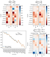 |
Fig. 2. Top left: fractional difference between TPB, 3 and TPB, 3∞ for the convergence maps and the shear catalogues with shape noise. Top right: fractional difference between TP5, 1h and TP5∞ for the convergence maps and the shear catalogues. TP5∞ does not include the two-halo term TP5, 2h as it is a finite-field term and therefore zero in the large-field approximation (Appendix A). Bottom left: relative contribution of the two-halo term TP5, 2h to the total TP5. The blue line for the shear catalogues and the orange line for the convergence maps of the SLICS. Bottom right: fractional difference between the analytical cross-covariance and its large-field approximation plus the two-halo term TP5, 2h for both datasets. |
4.3.2. Validation with N-body simulations
In Figs. 3 and 4, we compare the individual terms of the cross-covariance, both analytical and numerical, for the convergence maps and the shear catalogues, respectively. For all aperture radii combinations, TP5, 1h + TP5, 2h (which depends on the tetraspectrum) dominates. Furthermore, we observe that for almost all combinations, TPB, 2 is sub-dominant.
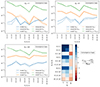 |
Fig. 3. Individual terms of the model cross-covariance, plotted together with the numerically measured ones of the SLICS without shape noise (convergence maps). The top left plot displays the terms when fixing θ4 = 4′, the top right when fixing θ4 = 8′, and the bottom left fixing θ4 = 16′. The bottom right heat map shows the difference between the modelled cross-covariance and the sample covariance normalised by the bootstrapping error. |
TP5 in general slightly over-predicts its numerical counterpart. The analytical TPB, 3 is marginally smaller than the numerical one for the convergence maps. Conversely, for the shear catalogues, we see that the analytical TPB, 3 is generally larger than the numerical one. The cause of the minor discrepancies between the numerical and analytical terms can be various. First, we expect the power-, bi-, and tetraspectrum to differ slightly in our model code and the SLICS simulation (see Appendix A in Heydenreich et al. 2023 for an example of the discrepancy between the measured and modelled bispectrum of the BiHalofit). This can be due to the binning, finite resolution, smoothing of the simulation fields, and uncertainties in Halofit and BiHalofit. Also, we describe TP5 with the halo model, which is an approximate model. Moreover, we only include the most significant contribution of the two-halo term. Taking these discrepancies into account, it can be stated that the numerical and analytical terms agree reasonably well. Only for the SLICS with shape noise, we see that the modelled TPB, 2 does not match the one measured from the simulation. This is probably due to the difficulties in measuring a finite-field term when noise is included. Taking the large-field approximation in Eq. (34) would mean neglecting  , after which the integral is, by definition, zero. That means the only reason it is non-zero for a finite field is the inclusion of
  . This function is a slowly varying function that leads to an amplification of the shape noise in the measured correlation functions. We, therefore, do not expect an exact match between the analytical and measured TPB, 2. Fortunately, as the finite-field term is sub-dominant, this has a negligible effect on the total cross-covariance. For the shear catalogues, we show the total analytical cross-covariance and the sample covariance, including error bars, in Fig. 4. The model cross-covariance is just the sum of the separate terms. It is seen that the tetraspectrum term almost exclusively determines it.
Also shown in the heat maps in Figs. 3 and 4 is the difference between the analytical cross-covariance and the sample covariance, normalised by the bootstrapping error. We observe that all filter combinations agree within 3.5σboot, with more than 50% lying within the 1σboot range. The model slightly over-predicts the sample covariance for most filter combinations, with the largest differences occurring for the smaller filter combinations. This is likely due to the differences mentioned earlier.
 |
Fig. 4. Individual terms of the analytical cross-covariance, plotted together with the numerically measured ones of the SLICS with shape noise (shear catalogues). The total analytical cross-covariance and the measured sample covariance are also plotted. The top left plot displays the terms when fixing θ4 = 4′, the top right when fixing θ4 = 8′, and the bottom left plot when fixing θ4 = 16′. The bottom right heat map shows the difference between the modelled cross-covariance and the sample covariance normalised by the bootstrapping error. |
5. Cosmological parameter estimation
With an analytical cross-covariance of the second- and third-order aperture mass statistics now available, we can combine it with the analytical covariances of  and
and  to form a joint covariance matrix. The left panel of Fig. 5 illustrates the fractional difference between the analytical and numerical joint covariance matrices for the SLICS with shape noise (shear catalogues). In this section, we compare the posterior distribution of S8 and Ωm obtained from the analytical joint covariance with those derived from the SLICS simulation with shape noise. We use a Markov Chain Monte Carlo (MCMC) sampling method for this comparison. It should be noted that the purpose of this paper is not to provide realistic estimates for either the clustering or the matter density parameter. Rather, this section aims to demonstrate that similar posterior distributions can be obtained from the analytical model when compared to the numerical posteriors. The posterior distribution of the analytical model is proportional to
 |
Fig. 5. Left: fractional difference between the analytical and numerical joint covariance matrix of the second- and third-order aperture mass statistics. The red lines divide the parts of the joint covariance matrix. The 3 × 3 matrix at the top left is the covariance matrix of |


![Mathematical equation: $$ \begin{aligned} P\left[m(\Theta )\,|\,d,\tilde{C}\right] \propto |\tilde{C}|^{-\frac{1}{2}} \,\mathrm{e}^{-\chi ^2/2}\; , \end{aligned} $$](/articles/aa/full_html/2025/10/aa54474-25/aa54474-25-eq68.gif) (42)
(42)
where m is the model vector containing the predicted values of ⟨ℳap⟩2(θi) and ⟨ℳap⟩3(θj, θk, θl) given the cosmological parameters Θ; d is the data vector, containing the measured second- and third-order aperture mass statistics; and  is the corresponding covariance matrix. For the numerical parameter estimation, we need to consider that we estimated the covariance from a finite sample. A correction for this is described in Percival et al. (2022). The numerical posterior distribution is proportional to
![Mathematical equation: $$ \begin{aligned} P\left[m(\Theta )\,|\,d,\tilde{C}\right] \propto |\tilde{C}|^{-\frac{1}{2}} \left( 1 + \frac{\chi ^2}{n_{\rm r}-1}\right)^{-m/2}\; , \end{aligned} $$](/articles/aa/full_html/2025/10/aa54474-25/aa54474-25-eq70.gif) (43)
(43)
where nr is the number of realisations. m is a power-law index
 (44)
(44)
nθ being the number of parameters Θ and nd the dimension of d. The χ2-distribution in Eqs. (42) and (43) is calculated as
![Mathematical equation: $$ \begin{aligned} \chi ^2 = \left[m(\Theta )-\boldsymbol{d}\right]^\mathrm{T} \tilde{C}^{-1} \left[m(\Theta )-d\right] \; . \end{aligned} $$](/articles/aa/full_html/2025/10/aa54474-25/aa54474-25-eq72.gif) (45)
(45)
We make our comparison by substituting  by Cjoint and
  , which are the analytical and numerical joint covariances, respectively, into Eqs. (42), (43), and (45). The numerical covariance
  is a positive definite matrix as it is calculated from the sample covariance. Our analytic covariance, as calculated to match the SLICS with shape noise, is not positive definite due to approximations and numerical errors, which poses a problem. Some of the subdominant eigenvalues of Cjoint are found to be negative. This leads to a χ2-distribution with a non-zero probability of finding negative χ2 values, leading to incorrect posterior distributions.
To mitigate this problem, we approximate our joint analytic covariance with a principal component analysis (PCA). This method corresponds to performing an eigendecomposition of the covariance matrix and cutting away the subdominant (negative) eigenvalues and the corresponding eigenvectors. Because our covariance matrix is ill-conditioned, meaning the eigenvalues are close to zero, numerical instability can arise in the eigendecomposition, causing issues in the accuracy of the eigenvalues and eigenvectors. These instabilities arise due to finite precision in computer calculations, causing small perturbations or rounding errors. A numerically more stable method is the singular value decomposition (SVD). It is a generalisation to the eigendecomposition and is theoretically equivalent for symmetric matrices. Performing an SVD factorises our covariance matrix
 (46)
(46)
where Σ is a matrix with the singular values on the diagonal in descending order (which correspond to the absolute values of the eigenvalues for a symmetric matrix), and U and VT are real matrices with orthonormal columns and rows, respectively. The diagonal matrix scales coordinates, and the matrices U and VT represent rotations and reflections of the space. Up to different signs per column, U and V are equivalent to the matrix of eigenvectors of Cjoint (but U and V are not the same; only the absolute values of the components are). We then cut away the diagonal terms corresponding to the negative eigenvalues and the corresponding columns and rows of U and VT, respectively. In our case, the original matrices are square 13 × 13 matrices. After the principal component analysis,  is a 13 × 10,
  a 10 × 10, and
  a 10 × 13 matrix (as we had three negative eigenvalues), where the tildes represent the matrices after the PCA, such that
 (47)
(47)
The new matrix  is a positive semi-definite matrix. As
  is a rank 10 matrix with dimensions 13 × 13, it is singular. Hence, it is non-invertible. Taking the inverse of the separate terms on the right-hand side of Eq. (47) is thus not possible as
  and
and  are not square matrices. Therefore, we take their pseudoinverse (denoted as a cross). As
  has orthonormal columns and
  orthonormal rows, their pseudoinverse matrices are equal to their transpose matrices (
 has an inverse, and thus the pseudoinverse is equal to the inverse)
 (48)
(48)
Substituting this approximation into Eq. (45), we find
![Mathematical equation: $$ \begin{aligned} \chi ^2 \approx \left[m(\Theta )-\boldsymbol{d}\right]^\mathrm{T} \tilde{V}\,\tilde{\Sigma }^{-1}\,\tilde{U}^\mathrm{T} \left[m(\Theta )-d\right] \; , \end{aligned} $$](/articles/aa/full_html/2025/10/aa54474-25/aa54474-25-eq89.gif) (49)
(49)
which has a strictly positive χ2-distribution. With this set-up, we perform a Metropolis-Hastings MCMC, trained on 6500 model points sampled in a Latin hypercube spanning the cosmological parameter space Ωm and S8. We use an emulator adopting the CosmoPower framework from Spurio Mancini et al. (2022) to efficiently compute the model predictions  and
and  (θj, θk, θl) for any given parameter vector Θ. The data vector d is constructed from the emulator evaluated at the fiducial cosmological parameters corresponding to the SLICS simulations. All other cosmological parameters not varied in the analysis are fixed to their SLICS values.
The right panel of Fig. 5 shows the analytical posterior contours for  ,
,  , and their joint posterior contour
  . The degeneracy directions of the second- and third-order aperture mass statistics differ noticeably, resulting in significantly tighter constraints when the two are combined. A comparison between the analytical and numerical S8 − Ωm contours is shown in the left panel of Fig. 6. We calculate the figure of merit (FoM) with a parameter covariance
  obtained from the MCMC process as
 |
Fig. 6. Posterior contours of S8 with Ωm obtained via MCMC. The blue contour is obtained via the sample covariance of the SLICS shear catalogues. The red contour is calculated via the analytical covariance. Left: using all the filter radii combinations in θ ∈ {4′,8′,16′}. Right: using only the combinations of θ ∈ {8′,16′}. |
 (50)
(50)
The fraction of the numerical over the analytical FoM is 0.72. The analytical posteriors are noticeably smaller than the numerical ones. In the left panel of Fig. 5, the largest discrepancies between the analytical and numerical cross-covariance occur at smaller filter radii scales (combinations with 4′). Therefore, we also perform an MCMC with combinations of 8′ and 16′ only, as shown in the right panel of Fig. 6. Excluding 4′, Cjoint does not contain any negative eigenvalues, so we did not perform a PCA. Here, the fraction of the numerical over the analytical FoM is 0.80, which is an improvement compared to when all filter radii combinations are included.
6. Discussion
We derived an analytical model for the non-tomographic cross-covariance between the real-space estimators  and
and  , and validated it against simulated data from SLICS, including both shape-noise-free convergence maps and shear catalogues with noise. The cross-covariance from the simulations was numerically determined through either the sample covariance or aperture mass correlation functions. For our selected set of aperture radii combinations, we found that the maximum deviation between the analytical and numerical results was 3.5 standard deviations on the bootstrapping uncertainty, with over 70% of the cases falling well within the two-sigma range. This was true for both datasets. The most likely cause of the discrepancies is a difference between the polyspectra used in the model and those from the simulation.
6.1. The large-field approximation
We find that the large-field approximation has a negligible effect on the terms TP5, 1h and TPB, 3. These can therefore be safely replaced by their large-field counterparts, TP5∞ and TPB, 3∞, for a SLICS sized or larger field, if a reduction in computational cost is desired or if the integration over the survey window function GA leads to numerical instability. The finite-field term TPB, 2 is consistently subdominant across the range of filter combinations tested. Its omission has little impact on the overall cross-covariance and it can be neglected without significantly affecting the result. In contrast, the finite-field term TP5, 2h is essential for achieving an accurate prediction. For combinations involving small aperture radii, it can contribute up to 60% of the total TP5, which is the dominant component of the cross-covariance. Neglecting this term would therefore lead to a substantial underestimation of the covariance at small scales. Since the amplitude of finite-field corrections decreases more rapidly than linearly with increasing survey area, their relevance is expected to diminish in Stage IV surveys. In particular, for significantly larger survey fields than those of SLICS, the contribution from TPB, 2 is negligible. Nonetheless, we recommend retaining TP5, 2h in any analysis that includes small-scale filters, even for larger-area surveys.
6.2. Analytical vs. numerical cross-covariance and origins of inaccuracy
The analytical cross-covariance model presented in this work agrees well with the numerical results from simulations across a broad range of filter combinations. For the configurations tested, 50% of the analytical predictions fall within the 1σ range of the bootstrap uncertainties, with the largest individual deviation reaching 3.5σ. The agreement is notably better for combinations involving larger aperture radii (16′), while the largest discrepancies arise at small filter scales. Testing the model at even larger aperture radii, such as 32′, in larger-volume simulations, for example, the full-sky GL simulations of Takahashi et al. (2017), would provide valuable insight into the behaviour of the analytic cross-covariance at lower ℓ and help isolate contributions from different model components.
There are several possible reasons for the observed discrepancies at smaller filter radii. The most significant source of inaccuracy is most likely the halo model used to compute the tetraspectrum term TP5, which dominates the cross-covariance at all aperture scales. Among its components, the two-halo contribution TP5, 2h is particularly impactful at small radii. As no more accurate tetraspectrum model is currently available, this approximation remains necessary, though the inclusion of additional two-halo contributions may improve the model’s fidelity, especially for the small filter scales, where TP5, 2h is dominant. While the power spectrum and bispectrum models used to compute TPB, 2 and TPB, 3 also differ from those implicit in the simulations, these terms are subdominant, typically by one to two orders of magnitude, and thus contribute less to the overall discrepancy.
A secondary limitation arises from numerical integration accuracy. The calculation of TP5 involves high-dimensional integrals that are computationally expensive and sensitive to binning. Due to performance constraints, we employed relatively coarse binning in parts of the integration, which limits the achievable precision. Some of the residual discrepancies are likely due to this numerical limitation.
Several other approximations were used in the model but are unlikely to contribute significantly to the observed discrepancies. First, the flat sky approximation was used. This is a valid approximation, as the scales probed in this are below ∼2°, where the induced error is negligible (Kilbinger et al. 2017). Moreover, this approximation was also applied in the simulations, meaning it cannot account for any discrepancies. However, it is important to consider this approximation when extending to larger fields, where larger filter radii can be probed, as it is expected to introduce greater errors at those scales. Additionally, the Limber approximation was used. This approximation becomes unreliable on scales larger than 6° (Deshpande & Kitching 2020). However, non-linear structure growth is minimal at these scales, meaning third-order statistics provide little additional information, making this limitation largely inconsequential.
In conclusion, the primary source of inaccuracy in the analytical cross-covariance model lies in the treatment of the tetraspectrum. Numerical integration precision contributes to a lesser extent, whereas other standard approximations, such as the flat-sky and Limber approximations, have a negligible impact on the angular scales considered.
6.3. Analytic vs. numerical cosmological inference
By combining the analytical cross-covariance derived here with the analytical  covariance of L+23 and the
  covariance of Linke et al. (2024), we constructed a joint analytical covariance matrix for use in cosmological parameter inference. We then compared its performance to the numerically derived covariance from SLICS in constraining the parameters Ωm and S8. The resulting constraints are broadly consistent between the two approaches. The analytical model yields slightly tighter confidence contours (Fig. 6), indicating slightly optimistic constraining power. However, interpreting this difference requires care, as the overall agreement of the covariance components is not uniform. The fractional difference matrix in the left panel of Fig. 5 shows that the analytical
  auto-covariance underpredicts its numerical counterpart, while both the cross-covariance and the
  auto-covariance tend to overpredict. This asymmetry suggests that the origin of the discrepancy in the contours is not easily attributable to a single term, such as the cross-covariance. In addition to the discrepancies for the cross-covariance mentioned before, a plausible explanation for the underpredicting
  auto-covariance lies in the modelling of the trispectrum. The analytical
  covariance includes a trispectrum term computed using only the one-halo contribution. If the trispectrum extracted from simulations (e.g. SLICS) is larger due to two-halo or higher-order contributions, this would lead to an underestimation of the variance in the analytical
  covariance, thereby shifting the contours accordingly. In contrast, the cross-covariance and
  covariance may slightly overpredict their counterparts due to different approximations or modelling assumptions.
In practice, the joint analytical covariance matrix is prone to numerical instability. Small-scale inaccuracies and inconsistencies among components can cause the matrix to become ill-conditioned, complicating operations such as matrix inversion. To mitigate this, PCA and SVD were applied to regularise the matrix. While PCA improves numerical stability, it also removes information from the data vector, leading to a slight degradation of the constraining power. These numerical issues highlight the sensitivity of cosmological inference to the stability and internal consistency of the covariance matrix, particularly when combining multiple orders of statistics. Future improvements to analytical models should aim not only for greater physical accuracy but also for improved numerical robustness.
6.4. Further comments
In realistic surveys, data often contain gaps due to masking, which prevents the direct computation of aperture mass statistics from convergence or shear maps using Eq. (6). Aperture centres located near masked regions lead to weighted integrals over incomplete areas, introducing biases in the aperture mass. To address this, the estimators ⟨ℳap2⟩ and ⟨ℳap3⟩ should instead be derived from their relations to the two- and three-point shear correlation functions (2PCF and 3PCF), as proposed by Schneider et al. (2005). However, even if masking is not explicitly accounted for, L+23 demonstrated that the analytical  covariance can still provide meaningful constraints by establishing upper and lower bounds. The upper bound is computed assuming a field size equal to the total unmasked survey area, while the lower bound excludes a boundary region equal to four times the largest aperture radius. For a SLICS-sized field, these bounds were found to be tight: the upper bound exceeded the lower bound by only ∼15%. In Stage IV surveys, the relative size of the excluded boundary will be smaller, implying even tighter bounds. Although we have not explicitly tested this for the analytical cross-covariance derived here, the underlying scaling arguments suggest that similar bounds should apply. This makes the analytical cross-covariance a practical tool even in the presence of realistic masking.
The analytical cross-covariance between  and
and  is closely related to the Fourier-space cross-covariance between the 3D power spectrum and bispectrum, as calculated by Sugiyama et al. (2020). While their formalism is three-dimensional, their approach closely parallels ours and can be translated to the 2D case via the Limber approximation. A direct comparison reveals that their expressions correspond to our large-field terms. Specifically, their Eq. (23) maps to our TPB, 3∞ and their Eq. (26) corresponds to our TP5∞. This correspondence is evident from the structural similarity of their k-space with our ℓ-space configurations. Sugiyama et al. (2020) note that their expressions do not include super-sample covariance (SSC) terms, which explains the absence of certain contributions. In Fourier space, SSC arises from modes larger than the survey area and must be added explicitly. In contrast, real-space calculations naturally incorporate these large-scale modes within the measured survey window, eliminating the need for separate SSC corrections. A detailed discussion of this distinction, and the implicit inclusion of SSC in real-space statistics, is provided in Linke et al. (2024).
6.5. Future work
One clear avenue for extending this work is the incorporation of tomography. A tomographic approach provides significantly more information on the evolution of large-scale structure and is particularly effective at reducing degeneracies between cosmological parameters such as Ωm and S8. It also enables meaningful constraints on a time-varying dark energy equation of state, w(z). However, extending the current model to a tomographic framework is non-trivial. It leads to a substantial increase in the size of both the data vector and the covariance matrix, which increases computational cost and the risk of numerical instability. Analytical derivation of the tomographic covariance is, however, still more feasible than relying on simulations, given the substantial resources required to generate tomographic mock catalogues, but it introduces new challenges for validation. In particular, as simulation-based benchmarks are often unavailable at high dimensionality, ensuring the numerical stability and internal consistency of tomographic analytical models remains a key difficulty.
While this work focused on the cross-covariance between aperture mass variance and skewness, the combination  is not the optimal choice for joint second- and third-order statistics in real data analyses. A primary limitation is that aperture mass statistics require knowledge of the two- and three-point correlation functions down to arbitrarily small angular separations and, formally, up to infinite separation. In practice, this is problematic as close galaxy pairs may be blended or lost to detection limits in real data and finite resolution and pixelisation prevent accurate small-scale correlation measurements in simulations. These limitations can lead to E-/B-mode leakage and loss of accuracy. A more robust alternative is to use COSEBIs (Complete Orthogonal Sets of E-/B-mode Integrals) for the second-order component (Schneider et al. 2010). COSEBIs are designed to operate over a finite angular range [θmin, θmax], with filter functions that are both complete and orthogonal. This ensures the mathematically exact separation of the E- and B-modes. While some residual leakage may occur due to numerical effects or masking, COSEBIs are considerably less sensitive to the limitations described above. Furthermore, COSEBIs offer a natural data compression: typically, the first 6 modes capture the majority of the cosmological information, even in tomographic analyses (Wright et al. 2025). A promising next step is therefore the development of an analytical cross-covariance between COSEBIs and
  , which would combine robustness, compactness, and sensitivity to non-Gaussian features. Additionally, second-order cosmic shear studies have also used the shear correlation functions ξ±, so a joint ξ± × ℳap3 covariance would also be a valuable extension.
6.6. Summary
In this work, we presented the first analytical real-space calculation of the cross-covariance between second- and third-order aperture mass statistics, completing the joint covariance matrix required for cosmological parameter estimation. For upcoming Stage IV surveys, analytical covariance matrices offer several advantages over simulation-based ones, including flexibility, scalability, and reduced noise. These benefits are most effectively realised when combined with COSEBIs for second-order statistics, and when extended to tomographic configurations. Nonetheless, limitations including the approximations inherent in the halo model, numerical instabilities in matrix operations, and difficulties in validation continue to hinder the broader adoption of analytical covariance matrices. Further developments are required to improve model accuracy, reduce numerical sensitivity, and enabling a tomographic set-up.
For the case  Eq. (A.11) in Heydenreich et al. (2020) has a factor 2 typo.
Acknowledgments
We would like to thank Joachim Harnois-Déraps for making public the SLICS mock data, which can be found at http://slics.roe.ac.uk/. We thank the anonymous referee for the useful comments. Funded by the TRA Matter (University of Bonn) as part of the Excellence Strategy of the federal and state governments. This work has been supported by the Deutsche Forschungsgemeinschaft through the project SCHN 342/15-1 and DFG SCHN 342/13. LL is supported by the Austrian Science Fund (FWF) [ESP 357-N]. PAB and SH acknowledge support from the German Academic Scholarship Foundation. LP acknowledges support from the DLR grant 50QE2002. SH is supported by the US Department of Energy, Office of High Energy Physics under Award Number DE-SC0019301.
References
- Asgari, M., Lin, C.-A., Joachimi, B., et al. 2021, A&A, 645, A104 [NASA ADS] [CrossRef] [EDP Sciences] [Google Scholar]
- Bartelmann, M. 2010, Class. Quant. Grav., 27, 233001 [CrossRef] [Google Scholar]
- Bartelmann, M., & Schneider, P. 2001, Phys. Rep., 340, 291 [Google Scholar]
- Burger, P., Friedrich, O., Harnois-Déraps, J., & Schneider, P. 2022, A&A, 661, A137 [NASA ADS] [CrossRef] [EDP Sciences] [Google Scholar]
- Burger, P. A., Porth, L., Heydenreich, S., et al. 2024, A&A, 683, A103 [NASA ADS] [CrossRef] [EDP Sciences] [Google Scholar]
- Cooray, A., & Sheth, R. 2002, Phys. Rep., 372, 1 [Google Scholar]
- Crittenden, R. G., Natarajan, P., Pen, U.-L., & Theuns, T. 2002, ApJ, 568, 20 [NASA ADS] [CrossRef] [Google Scholar]
- Dalal, R., Li, X., Nicola, A., et al. 2023, Phys. Rev. D, 108, 123519 [CrossRef] [Google Scholar]
- DES Collaboration 2022, Phys. Rev. D, 105, 023520 [CrossRef] [Google Scholar]
- Deshpande, A. C., & Kitching, T. D. 2020, Phys. Rev. D, 101, 103531 [NASA ADS] [CrossRef] [Google Scholar]
- Di Valentino, E., Anchordoqui, L. A., Özgür, A., et al. 2021, Astropart. Phys., 131, 102604 [NASA ADS] [CrossRef] [Google Scholar]
- Euclid Collaboration (Ajani, V., et al.) 2023, A&A, 675, A120 [NASA ADS] [CrossRef] [EDP Sciences] [Google Scholar]
- Euclid Collaboration (Mellier, Y., et al.) 2025, A&A, 697, A1 [Google Scholar]
- Falco, E. E., Gorenstein, M. V., & Shapiro, I. I. 1985, ApJ, 289, L1 [Google Scholar]
- Gruen, D., Friedrich, O., Krause, E., et al. 2018, Phys. Rev. D, 98, 023507P [Google Scholar]
- Harnois-Déraps, J., & van Waerbeke, L. 2015, MNRAS, 450, 2857 [Google Scholar]
- Harnois-Déraps, J., Amon, A., Choi, A., et al. 2018, MNRAS, 481, 1337 [Google Scholar]
- Harnois-Déraps, J., Martinet, N., Castro, T., et al. 2021, MNRAS, 506, 1623 [CrossRef] [Google Scholar]
- Heydenreich, S., Schneider, P., Hildebrandt, H., et al. 2020, A&A, 634, A104 [NASA ADS] [CrossRef] [EDP Sciences] [Google Scholar]
- Heydenreich, S., Brück, B., & Harnois-Déraps, J. 2021, A&A, 648, A74 [NASA ADS] [CrossRef] [EDP Sciences] [Google Scholar]
- Heydenreich, S., Linke, L., Burger, P., & Schneider, P. 2023, A&A, 672, A44 [NASA ADS] [CrossRef] [EDP Sciences] [Google Scholar]
- Heymans, C., Tröster, T., Asgari, M., et al. 2021, A&A, 646, A140 [NASA ADS] [CrossRef] [EDP Sciences] [Google Scholar]
- Hildebrandt, H., Viola, M., Heymans, C., et al. 2017, MNRAS, 465, 1454 [Google Scholar]
- Hoekstra, H., & Jain, B. 2008, Ann. Rev. Nucl. Part. Sci., 58, 99 [NASA ADS] [CrossRef] [Google Scholar]
- Joudaki, S., Hildebrandt, H., Traykova, D., et al. 2020, A&A, 638, L1 [NASA ADS] [CrossRef] [EDP Sciences] [Google Scholar]
- Kaiser, N., & Jaffe, A. 1997, ApJ, 484, 545 [NASA ADS] [CrossRef] [Google Scholar]
- Kayo, I., Takada, M., & Jain, B. 2013, MNRAS, 429, 344 [Google Scholar]
- Kilbinger, M., & Schneider, P. 2005, A&A, 442, 69 [NASA ADS] [CrossRef] [EDP Sciences] [Google Scholar]
- Kilbinger, M., Heymans, C., Asgari, M., et al. 2017, MNRAS, 472, 2126 [Google Scholar]
- Laureijs, R., Amiaux, J., Arduini, S., et al. 2011, ArXiv e-prints [arXiv:1110.3193] [Google Scholar]
- Limber, D. N. 1954, ApJ, 119, 655 [NASA ADS] [CrossRef] [Google Scholar]
- Linke, L., Heydenreich, S., Burger, P. A., & Schneider, P. 2023, A&A, 672, A185 [NASA ADS] [CrossRef] [EDP Sciences] [Google Scholar]
- Linke, L., Burger, P. A., Heydenreich, S., Porth, L., & Schneider, P. 2024, A&A, 681, A33 [NASA ADS] [CrossRef] [EDP Sciences] [Google Scholar]
- Martinet, N., Schneider, P., Hildebrandt, H., et al. 2018, MNRAS, 474, 712 [Google Scholar]
- Percival, W. J., Friedrich, O., Sellentin, E., & Heavens, A. 2022, MNRAS, 510, 3207 [NASA ADS] [CrossRef] [Google Scholar]
- Planck Collaboration VI. 2020, A&A, 641, A6 [NASA ADS] [CrossRef] [EDP Sciences] [Google Scholar]
- Porth, L., Heydenreich, S., Burger, P., Linke, L., & Schneider, P. 2024, A&A, 689, A227 [NASA ADS] [CrossRef] [EDP Sciences] [Google Scholar]
- Pyne, S., & Joachimi, B. 2021, MNRAS, 503, 2300 [NASA ADS] [CrossRef] [Google Scholar]
- Schneider, P. 1996, MNRAS, 283, 837 [Google Scholar]
- Schneider, P., & Lombardi, M. 2003, A&A, 397, 809 [NASA ADS] [CrossRef] [EDP Sciences] [Google Scholar]
- Schneider, P., & Seitz, C. 1995, A&A, 294, 411 [NASA ADS] [Google Scholar]
- Schneider, P., Kilbinger, M., & Lombardi, M. 2005, A&A, 431, 9 [NASA ADS] [CrossRef] [EDP Sciences] [Google Scholar]
- Schneider, P., Eifler, T., & Krause, E. 2010, A&A, 520, A116 [NASA ADS] [CrossRef] [EDP Sciences] [Google Scholar]
- Sheth, R. K., & Tormen, G. 1999, MNRAS, 308, 119 [Google Scholar]
- Spurio Mancini, A., Piras, D., Alsing, J., Joachimi, B., & Hobson, M. P. 2022, MNRAS, 511, 1771 [NASA ADS] [CrossRef] [Google Scholar]
- Sugiyama, N. S., Saito, S., Beutler, F., & Seo, H.-J. 2020, MNRAS, 497, 1684 [Google Scholar]
- Takada, M., & Jain, B. 2004, MNRAS, 348, 897 [Google Scholar]
- Takahashi, R., Sato, M., Nishimichi, T., Taruya, A., & Oguri, M. 2012, ApJ, 761, 152 [Google Scholar]
- Takahashi, R., Hamana, T., Shirasaki, M., et al. 2017, ApJ, 850, 24 [Google Scholar]
- Takahashi, R., Nishimichi, T., Namikawa, T., et al. 2020, ApJ, 895, 113 [NASA ADS] [CrossRef] [Google Scholar]
- Wright, A. H., Stölzner, B., Asgari, M., et al. 2025, A&A, in press, https://doi.org/10.1051/0004-6361/202554908 [Google Scholar]
Appendix A: The tetraspectrum halo model
In this appendix, we approximate the tetraspectrum using a halo model as in Cooray & Sheth (2002). The purpose of this estimation is to model TP5 (Eq. 24), which can be slightly modified and expressed as
 (A.1)
(A.1)
where s = ℓ1+ ℓ2+ ℓ3 was used, such that the geometry factor only depends on a single input value. The tetraspectrum of the convergence is given by the Limber integration (Eq. 5),
 (A.2)
(A.2)
where the tetraspectrum of the density contrast can be decomposed into terms that include up to five halos. Specifically, the one-halo term corresponds to all five points in the correlation function lying within a single halo, while the two-halo term involves the points being distributed between two halos. As a result, the tetraspectrum of the density contrast can be expressed as
 (A.3)
(A.3)
where  is the linear density contrast power spectrum, and the Inl terms are defined as
![Mathematical equation: $$ \begin{aligned} I^l_n(k_1, ..., k_n; \chi ) = \int \mathrm{d} m\; n\left[m,z(\chi )\right]\, \left(\frac{m}{\bar{\rho }}\right)^n\, b^l\left[m,z(\chi )\right]\, \prod _{i = 1}^n\, \tilde{u}_{\rm NFW}(k_i,m)\; , \end{aligned} $$](/articles/aa/full_html/2025/10/aa54474-25/aa54474-25-eq119.gif) (A.4)
(A.4)
where m is the halo mass, n(m, z) is the halo mass function from Sheth & Tormen (1999),  is the comoving mean density, b(m, z) the halo bias (Sheth & Tormen 1999), and
  is the Fourier transformed and normalised Navarro–Frenk–White-halo profile, which is defined as uNFW(r, m) = ρ(r, m)/m, where ρ is the halo density profile. We note that when Inl terms are multiplied (meaning multiple halos), the masses, and thus also the integrations, are distinct per halo.
As the distance between halos is much greater than within one halo, the one-halo term will dominate on small scales (large ℓ/χ). However, in the one-halo term, we only have correlations up to the scale of the largest halo. Therefore, we expect the one-halo term to be subdominant on scales larger than halos. It is shown in Pyne & Joachimi (2021), that on large scales, in the assumption that s ≪ ℓ1, ℓ2, ℓ4, the two-halo term depending on  dominates. Therefore, we can approximate Eq. (A.3) as
 (A.5)
(A.5)
where in the second approximation, we neglected s except for in the linear power spectrum, as  . Now, filling in this approximation into Eq. (A.1), and using isotropy, yields
![Mathematical equation: $$ \begin{aligned} T_{\rm P5}(\theta _1,\theta _2,\theta _3;\theta _4)\approx&\; \left(\frac{3H_0^2\Omega _{\rm m}}{2c^2}\right)^5\,\int \frac{\mathrm{d}^2\ell _1}{(2\pi )^2}\int \frac{\mathrm{d}^2\ell _2}{(2\pi )^2} \int \frac{\mathrm{d}^2s}{(2\pi )^2} \int \frac{\mathrm{d}^2\ell _4}{(2\pi )^2} \,\int _0^\infty \mathrm{d}{\chi }\; \frac{q^5(\chi )}{\chi ^{3}\, a(\chi )^5} \nonumber \\&\times \tilde{u}(\ell _1 \theta _1) \, \tilde{u}(\ell _2 \theta _2) \, \tilde{u}(|\ell _1 + \ell _2|\ \theta _3) \, \tilde{u}(\ell _4 \theta _4) \, \tilde{u}(\ell _4 \, \theta _4) \, G_A(s) \nonumber \\&\times \left[I^\mathrm{0}_{\rm 5}(\ell _1/\chi , \ell _2/\chi ,|\ell _1+\ell _2|/\chi ,\ell _4/\chi , \ell _4/\chi ; \chi ) + P_{\rm L}^\mathrm{(3d)}(s/\chi )\, I^\mathrm{1}_{\rm 3}(\ell _1/\chi , \ell _2/\chi , |\ell _1+\ell _2|/\chi ;\chi )\, I^\mathrm{1}_{\rm 2}(\ell _4/\chi ,\ell _4/\chi ; \chi )\right] \\ =&\; T_{\rm P5,1h}(\theta _1,\theta _2,\theta _3;\theta _4)+T_{\rm P5,2h}(\theta _1,\theta _2,\theta _3;\theta _4)\; , \nonumber \end{aligned} $$](/articles/aa/full_html/2025/10/aa54474-25/aa54474-25-eq125.gif) (A.6)
(A.6)
where
![Mathematical equation: $$ \begin{aligned} T_{\rm P5,2h}(\theta _1,\theta _2,\theta _3;\theta _4)&=\left(\frac{3H_0^2\Omega _{\rm m}}{2c^2}\right)^5\,\int _0^\infty \mathrm{d}{\chi }\; \frac{q^5(\chi )}{\chi ^{3}\, a(\chi )^5} \left[\int \frac{\mathrm{d}^2s}{(2\pi )^2}\,G_A(s) \, P_{\rm L}^\mathrm{(3d)}(s/\chi )\right]\,\int \frac{\mathrm{d}^2\ell _1}{(2\pi )^2}\int \frac{\mathrm{d}^2\ell _2}{(2\pi )^2} \int \frac{\mathrm{d}^2\ell _4}{(2\pi )^2} \; \nonumber \\&\quad \times \tilde{u}(\ell _1 \theta _1) \, \tilde{u}(\ell _2 \theta _2) \, \tilde{u}(|\ell _1 + \ell _2|\ \theta _3) \, \tilde{u}(\ell _4 \theta _4) \, \tilde{u}(\ell _4 \, \theta _4) \, I^\mathrm{1}_{\rm 3}(\ell _1/\chi , \ell _2/\chi , |\ell _1+\ell _2|/\chi ;\chi )\, I^\mathrm{1}_{\rm 2}(\ell _4/\chi ,\ell _4/\chi ; \chi ) \end{aligned} $$](/articles/aa/full_html/2025/10/aa54474-25/aa54474-25-eq126.gif) (A.7)
(A.7)
will be zero in the large-field limit, where the integration over the Dirac delta function in Eq. (25) gives us a factor  . Thus, we find a finite-field term similar to TPB, 2.
All Tables
All Figures
|
Fig. 1. Aperture centre placement in a data field (from L+23). Given a data field of area A′ (not necessarily a square field), apertures are only placed within a smaller field A, which lies well within A′. The boundary of A is chosen such that 99.9% of the effective support of Qθ lies within A (which corresponds to ∼4 θ) if the aperture centre lies on this boundary. To illustrate this, two aperture centres are depicted: ϕ is within A and ϕ″ is outside of A. It can be seen that the circle around ϕ″, illustrating the effective support of Qθ, extends beyond A′, thus introducing bias into the calculated aperture mass at this point. To exclude this effect, we only average the aperture centre over the red region A. |
| In the text | |
|
Fig. 2. Top left: fractional difference between TPB, 3 and TPB, 3∞ for the convergence maps and the shear catalogues with shape noise. Top right: fractional difference between TP5, 1h and TP5∞ for the convergence maps and the shear catalogues. TP5∞ does not include the two-halo term TP5, 2h as it is a finite-field term and therefore zero in the large-field approximation (Appendix A). Bottom left: relative contribution of the two-halo term TP5, 2h to the total TP5. The blue line for the shear catalogues and the orange line for the convergence maps of the SLICS. Bottom right: fractional difference between the analytical cross-covariance and its large-field approximation plus the two-halo term TP5, 2h for both datasets. |
| In the text | |
|
Fig. 3. Individual terms of the model cross-covariance, plotted together with the numerically measured ones of the SLICS without shape noise (convergence maps). The top left plot displays the terms when fixing θ4 = 4′, the top right when fixing θ4 = 8′, and the bottom left fixing θ4 = 16′. The bottom right heat map shows the difference between the modelled cross-covariance and the sample covariance normalised by the bootstrapping error. |
| In the text | |
|
Fig. 4. Individual terms of the analytical cross-covariance, plotted together with the numerically measured ones of the SLICS with shape noise (shear catalogues). The total analytical cross-covariance and the measured sample covariance are also plotted. The top left plot displays the terms when fixing θ4 = 4′, the top right when fixing θ4 = 8′, and the bottom left plot when fixing θ4 = 16′. The bottom right heat map shows the difference between the modelled cross-covariance and the sample covariance normalised by the bootstrapping error. |
| In the text | |
|
Fig. 5. Left: fractional difference between the analytical and numerical joint covariance matrix of the second- and third-order aperture mass statistics. The red lines divide the parts of the joint covariance matrix. The 3 × 3 matrix at the top left is the covariance matrix of |
| In the text | |
|
Fig. 6. Posterior contours of S8 with Ωm obtained via MCMC. The blue contour is obtained via the sample covariance of the SLICS shear catalogues. The red contour is calculated via the analytical covariance. Left: using all the filter radii combinations in θ ∈ {4′,8′,16′}. Right: using only the combinations of θ ∈ {8′,16′}. |
| In the text | |
Current usage metrics show cumulative count of Article Views (full-text article views including HTML views, PDF and ePub downloads, according to the available data) and Abstracts Views on Vision4Press platform.
Data correspond to usage on the plateform after 2015. The current usage metrics is available 48-96 hours after online publication and is updated daily on week days.
Initial download of the metrics may take a while.