| Issue |
A&A
Volume 702, October 2025
|
|
|---|---|---|
| Article Number | A120 | |
| Number of page(s) | 12 | |
| Section | Cosmology (including clusters of galaxies) | |
| DOI | https://doi.org/10.1051/0004-6361/202554621 | |
| Published online | 14 October 2025 | |
Emulating the non-linear matter power spectrum in mixed axion dark matter models
Institute of Theoretical Astrophysics, University of Oslo, PO Box 1029 Blindern, 0315 Oslo, Norway
⋆ Corresponding author: This email address is being protected from spambots. You need JavaScript enabled to view it.
Received:
18
March
2025
Accepted:
12
August
2025
Abstract
In order to constrain ultra light dark matter models with current and near future weak lensing surveys, we need the predictions for the non-linear dark matter power spectrum. This is commonly extracted from numerical simulations or from semi-analytical methods. For ultra light dark matter models, such numerical simulations are often very expensive due to the need of having a very high force resolution, often limiting the simulations to very small simulation boxes that do not contain very large scales. In this work, we take a different approach by relying on fast approximate N-body simulations. In these simulations, axion physics is only included in the initial conditions, allowing us to run a large number of simulations with varying axion and cosmological parameters. From our simulation suite, we used machine learning tools to create an emulator for the ratio of the dark matter power spectrum in mixed axion models – models where dark matter is a combination of CDM and axion – to that of ΛCDM. The resulting emulator only needs to be combined with existing emulators for ΛCDM to be able to be used in parameter constraints. We compared the emulator to semi-analytical methods, but a more thorough test to full simulations to verify the true accuracy of this approach is not possible at the present time and is left for future work.
Key words: dark matter / large-scale structure of Universe
© The Authors 2025
 Open Access article, published by EDP Sciences, under the terms of the Creative Commons Attribution License (https://creativecommons.org/licenses/by/4.0), which permits unrestricted use, distribution, and reproduction in any medium, provided the original work is properly cited.
This article is published in open access under the Subscribe to Open model. This email address is being protected from spambots. You need JavaScript enabled to view it. to support open access publication.
1. Introduction
Cold dark matter (CDM), which is thought to be a weakly interacting massive particle (WIMP), is the current leading candidate for dark matter. It successfully describes a number of observations, such as the internal dynamics of galaxy clusters (Zwicky 1937; Clowe et al. 2006), the rotation curve of spiral galaxies (Rubin et al. 1980; Persic et al. 1996), and the weak gravitational lensing effects produced by large-scale matter structures (Mateo 1998; Heymans et al. 2013; Planck Collaboration XV 2016). However, the search for CDM through indirect astronomical measurements (Albert et al. 2017), direct laboratory experiments (Danninger 2017), and high-energy collider experiments (Buonaura 2017) has not yielded any conclusive evidence for dark matter in the GeV range.
Additionally, some discrepancies between observations and simulations of CDM around k ∼ 10 kpc−1 scales may suggest that the CDM model is insufficient when it comes to describing sub-halo structures. One such discrepancy, which has become known as the cusp-core problem (Oh et al. 2011; de Blok 2009), is the observation of relatively flat density profiles toward the center of dark matter halos (Walker & Peñarrubia 2011), whereas N-body simulations suggest an increasing profile (Navarro et al. 1996). Another discrepancy is the missing satellite problem (Klypin et al. 1999; Moore et al. 1999), where N-body simulations predict a much higher abundance of satellite galaxies than what is found in observations. Although these issues could be explained by an imperfect implementation of baryonic physics in numerical simulations (Macciò et al. 2012), some studies claim that these issues persist even when accounting for small scale baryonic physics (Pawlowski et al. 2015; Sawala et al. 2014). These discrepancies sparked the search for alternative dark matter models that behave differently from CDM on galactic scales, while still being successful on cosmological scales.
One such model is the axion, an extremely light boson originally proposed by string theory (Arvanitaki et al. 2010). This form of dark matter belongs to a suite of wave-like dark matter also known as fuzzy dark matter (or ψDM). Axions form a non-relativistic Bose-Einstein condensate, which means that the uncertainty principle leads to a self-interacting pressure. This pressure counteracts gravity on scales smaller than the Jeans scale (Schive et al. 2014). As a result, on these smaller scales, perturbations oscillate rather than grow. However, on larger scales, axions behave in the same way as CDM (Schive et al. 2016). This makes them an attractive dark matter model, as they might alleviate discrepancies on galactic scales without altering large-scale structure formation.
The evolution of the axions follows the Schrödinger-Poisson equations, which can be solved using high-resolution adaptive mesh refinement (AMR) algorithms (Schive et al. 2018). While this approach leads to impressive results in terms of resolution (Schive et al. 2014; Woo & Chiueh 2009), it is highly resource-intensive, making it impractical for including a full hydrodynamic description of gas and star formation in cosmologically representative simulation domains. One way to reduce the computational demand is by incorporating the dynamical effect of quantum pressure via smoothed particle hydrodynamics (SPH), allowing for less intensive simulations without sacrificing cosmological results (Nori & Baldi 2018). Another approach is to use standard N-body codes and include the effects of axions only in the initial conditions, thereby neglecting axion physics in the simulations (Iršič et al. 2017; Schive et al. 2016; Armengaud et al. 2017).
The standard approach to inferring cosmological parameters, including those related to axions, is through Bayesian techniques. However, approaches that rely on generating numerous accurate theoretical predictions, such as a Markov chain Monte Carlo (MCMC) approach, quickly become computationally expensive due to the need for many N-body simulations. A promising approach that may alleviate the numerical load is the use of emulators, which can model the relation between cosmological parameters and observables such as the power spectrum. Some examples of cosmological emulators include EUCLIDEMULATOR1, EUCLIDEMULATOR2 (Knabenhans et al. 2019, 2021), FRANKENEMU (Heitmann et al. 2013), DARK QUEST (Nishimichi et al. 2019), and the BACCO emulator (Angulo et al. 2021).
In this paper, we use a fast approximate N-body simulation known as the Comoving Lagrangian Acceleration (COLA) method to simulate the axions as standard CDM particles, where the axion physics only come into play in the initial conditions. These initial conditions are generated using AXIONCAMB (Hlozek et al. 2015), where the axion mass and the axion abundance, that is the fraction of the total dark matter energy budget that consists of axions, are free parameters. Using this approach, we generated a data set that we used to train an emulator that quickly estimates the non-linear matter power spectrum with axions.
Our aim is to provide an emulator that can be used to constrain the combined cosmological and axion parameters. This may be achieved through weak-lensing surveys, such as the Deep Lensing Survey (DLS; Wittman et al. 2002), the Canada–France–Hawaii Telescope Lensing Survey (CFHTLS; Heymans et al. 2013), the Kilo-Degree Survey (KiDS; de Jong et al. 2013), the Dark Energy Survey (DES; Dark Energy Survey Collaboration 2016), and the Legacy Survey of Space and Time (LSST; The LSST Dark Energy Science Collaboration 2021), which directly probe the combined abundance of baryons and dark matter. Combined with a ΛCDM emulator, our emulator can make predictions for the matter power spectrum with mixed axion dark matter, which can be used to predict the angular power spectrum of convergence and shear extracted from weak-lensing surveys. This makes it possible to make constraints through bayesian statistical methods, such as MCMC.
The setup of this paper is as follows: In Sect. 2 we review the axion model and discuss different methods for performing simulations. We also discuss semi-analytical methods for predicting the non-linear matter power spectrum and review existing constraints on the axion mass and axion fraction. In Sect. 3 we describe our simulation setup, and in Sect. 4 we describe how we created our emulator. In Sect. 5 we compare the results of our simulations to linear theory and semi-analytical methods before concluding in Sect. 6.
2. Theory
In this section we review the basics of mixed axion models from its formulation, background evolution, perturbations, and simulations. We also discuss semi-analytical methods for predicting the power spectrum.
2.1. Background cosmology
The action for an axion scalar field is
![Mathematical equation: $$ \begin{aligned} S = \int d^4x\sqrt{-g}\left[\frac{1}{2}g^{\mu \nu }\partial _\mu \phi \partial _\nu \phi - \frac{1}{2}m_{\rm ax}^2\phi ^2\right], \end{aligned} $$](/articles/aa/full_html/2025/10/aa54621-25/aa54621-25-eq1.gif) (1)
(1)
and it gives rise to the equation of motion (the Klein-Gordon equation)
 (2)
(2)
where
 (3)
(3)
is the d’Alembert operator. At the zeroth order, Eq. (2) describes the cosmological background of the axion field and takes the form of a damped harmonic oscillator (Marsh 2016). The equation is given by
 (4)
(4)
When 3H ≫ max, the field is over-damped and essentially “frozen”. This causes the axions to fulfill the slow-roll condition, making them behave similar to dark energy. Once max ∼ 3H, the field begins to oscillate, and the axions begin to behave as dark matter. To see this more clearly, in a matter or radiation dominated Universe, a ∝ an, and the solution is given by
![Mathematical equation: $$ \begin{aligned} \phi = a^{-3/2} (t/t_{\rm ini})^{1/2}[A J_\ell (mt) + B Y_\ell (mt)], \end{aligned} $$](/articles/aa/full_html/2025/10/aa54621-25/aa54621-25-eq5.gif) (5)
(5)
where Jm, Ym are Bessel-functions; tini is the initial time; ℓ = (3n − 1)/2; and A, B are set by the initial conditions. The energy density and pressure of the axion field are given by
 (6)
(6)
 (7)
(7)
Averaged over time, the solution above, for max ≫ 3H, leads to ρ ∝ a−3 and P ≈ 0, and the axion behaves as dark matter. In the late Universe and for the axion masses of interest for us (10−22 eV–10−28 eV), the background evolution will be practically the same as that for ΛCDM.
2.2. Numerical simulations of axions
In the non-relativistic limit, we can expand Eq. (2) in terms of a complex field ψ using the Wentzel-Kramers-Brillouin (WKB) ansatz,
 (8)
(8)
This factors out some of the oscillations (e±imaxt) experienced by the axions. The complex field ψ then follows the Schrödinger equation
 (9)
(9)
with ΦN as the Newtonian potential, given by the Poisson equation
![Mathematical equation: $$ \begin{aligned} \nabla ^2\Phi _{\rm N} = 4 \pi G a^2 \left[m_{\rm ax}(|\psi |^2 - \langle |\psi |\rangle ^2) + \delta \rho _f \right]. \end{aligned} $$](/articles/aa/full_html/2025/10/aa54621-25/aa54621-25-eq10.gif) (10)
(10)
In Eq. (10), |ψ|2 − ⟨|ψ|⟩2 serves as the overdensity δρax for the Axion scalar field, while δρf describes the overdensity of CDM and baryons.
An alternative description of the axion fluid is provided by the so-called Madelung formulation of the Schrödinger equation. Defining  and v = ∇θ/m, Eq. (9) can then be written as the fluid equations
 (11)
(11)
 (12)
(12)
where  . This is the well-known continuity and Euler equation (for an irrotational fluid ∇ × v = 0) where Q acts as a pressure term, commonly called the quantum pressure. Even though the equations describe an irrotational fluid, in the region where ρ → 0, the phase can develop discontinuities that again can generate vorticity in the field.
These different formulations mentioned above give rise to different approaches of simulating the axion. One such approach is the operator splitting technique with finite differencing, where the wave function is advanced in time by applying a unitary transformation:
 (13)
(13)
The last (kinetic) operator is computed by Taylor expanding it and evaluating the resulting terms ∇2nψ using finite difference. The main advantage of this method is that it generalizes to a non-uniform mesh. This was the original approach of Schive et al. (2014) and was later implemented in the SCALAR code (Mina et al. 2020).
A closely related approach is the pseudo-spectral method, which also relies on operator splitting but evaluates the kinetic operator in Fourier space, i.e.:
![Mathematical equation: $$ \begin{aligned} e^{\frac{i}{2m}\Delta t \nabla ^2}\psi (x,t) = \mathcal{F} ^{-1}[e^{-\frac{i}{2m}\Delta t k^2}\mathcal{F} [\psi (x,t)]], \end{aligned} $$](/articles/aa/full_html/2025/10/aa54621-25/aa54621-25-eq16.gif) (14)
(14)
where ℱ denotes the Fourier transform. The advantage of this method is that it is very accurate, but it requires us to have a full grid. To get high resolution, the box size either needs to be small or the number of grid cells needs to be very large. This is the approach taken by, for example, May & Springel (2021, 2023).
Another distinct approach is to use the Madelung formulation and simulate the axions using smoothed particle hydrodynamics (SPH). Here, the axions are modeled as tracer particles, from which one can estimate the density and quantum pressure to evolve the equations. This approach is taken by AX-GADGET (Nori & Baldi 2018).
Finally, with hybrid methods, one can combine the use of the pseudo-spectral method on the root grid with finite differencing on adaptively refined grids. This is the approach taken by AxioNyx (Schwabe et al. 2020).
The main issue with most of these methods is that since the Schrödinger equation is first order in time and second order in space, the stability is only guaranteed when Δt ≲ (Δx)2. In addition to this the spatial resolution Δx should satisfy Δx ≲ λdB, the de-Brouigle wavelength of the axion, which typically is very small 𝒪(kpc). This means that we need very fine grids and very small time steps, making the simulations very costly. This issue is avoided for the SPH approach, as there is no underlying mesh, but it still requires fine time steps. However, for this method, there is also the question if it really can produce all the wave-like behavior we get when solving the Schrödinger equation.
For this reason, most of the simulations done so far have restricted themselves to very small simulation boxes B = 𝒪(1 − 15 Mpc). Many of these simulations have also not been simulated all the way to redshift z = 0, but rather ending at a higher redshift.
The approach we take in this paper is the most naive one: We simply include the effect of the axion, as predicted by linear perturbation theory, only in the initial conditions. This ignores the effect of the quantum pressure, but do allow us to simulate large cosmological boxes.
It is hard to properly assess the accuracy of our approach, as there are few big-box simulations available in the literature. For simulations using the Madelung formulation there have been simulations (with a box size of 10 − 15 Mpc/h) performed with and without including the quantum pressure and a very good agreement was found when it comes to the matter power spectrum (see, e.g., Fig. 9 in Nori & Baldi 2018). In Veltmaat & Niemeyer (2016) it was shown that cosmological simulations (with a box size of 2 Mpc/h) including the quantum pressure gives rise to a maximum relative difference of 10% in the power spectrum near the quantum Jeans length, below which gravitational growth of perturbations is suppressed. All these simulations were for an axion abundance, fax ≡ Ωax/(Ωax + ΩCDM), of fax = 1 and we would expect differences to diminish with decreasing axion abundance.
2.3. The halo model and the AXIONHMCODE prediction
The halo model (Seljak 2000) assumes that all the matter in the Universe is located inside halos. With this assumption, the 2-point correlation function can then be written analytically as the sum of two terms: first, we have the 2-halo term, P2h, which takes into account the correlations between mass-elements in two different halos; and second, the 1-halo term, P1h, which takes into account correlations between mass-elements within the same halo. For the power spectrum, this gives us
 (15)
(15)
![Mathematical equation: $$ \begin{aligned} P_{\rm 2h}(k)&= P_{\rm lin}(k)\left[\frac{1}{\overline{\rho }_m}\int \frac{\mathrm{d}n}{\mathrm{d}\log M} b(M)y(k,M) \mathrm{d}M\right]^2,\end{aligned} $$](/articles/aa/full_html/2025/10/aa54621-25/aa54621-25-eq18.gif) (16)
(16)
 (17)
(17)
where Plin(k) is the linear dark matter power spectrum, b(M) is the halo-bias, dn/dlog M is the halo mass-function, and y(k, M) is the Fourier transform of the halo density profile ρ(r, M). The 2-halo term dominates the prediction on large scales (small k), while the 1-halo term dominates on small-scales.
The ingredients needed to evaluate the halo model are the density profile ρ(M), the mass-function dn/dlog M and the bias b(M). The latter two are for ΛCDM often taken to be the analytical fit made by Sheth-Tormen (Sheth et al. 2001) and for the former it is most often taken to be a NFW profile with a mass-concentration relation, c(M), derived from simulations.
For axions all these ingredients are expected to change. First of all, the density profile will in general be cored and the mass-function will have a cutoff for small masses. Another complication that arises when we consider mixed dark matter models, where only part of the DM budget is in the form of axions and the rest in the form of CDM. This leads to a prediction:
 (18)
(18)
where each of the terms above can be computed in the halo-model, and the full equations can be found in Vogt et al. (2023). This is implemented in the AXIONHMCODE package1 (Vogt et al. 2023) and includes improvements to the model by calibrating it to axion simulations as performed in Dome et al. (2024).
AXIONHMCODE takes into account the cutoff in the halo mass-function and uses a solitonic core for the axion density profile (derived from the simulations of Schive et al. 2014):
 (19)
(19)
where rc is the core radius defined as where the density drops to one half of the central density and has been found to be well approximated by (Schive et al. 2014),
 (20)
(20)
where Δv(z) is the halo virial overdensity. The AXIONHMCODE approach includes all the physics we expect to be present in mixed axion DM models, except for the presence of interference patterns. However, these are small-scale effects and are only expected to lead to modifications on very small scales beyond what we are interested in modeling with the power spectrum. In the absence of simulations with large boxes to compare, we use this package as the main comparison throughout this paper.
2.4. Existing cosmological constraints
Axions alter the expansion history and growth of perturbations in ways that are observable in the cosmic microwave background (CMB). Specifically, the introduction of axions have two distinguishing features that pertains to cosmological observables (Hlozek et al. 2015). Firstly, when the axion field rolls slowly, it leads to a background evolution that is equivalent with a portion of the matter component behaving as an early form of dark energy. One result of this is that the early-time integrated Sachs-Wolfe (ISW) effect is modified and the positions and amplitudes of acoustic peaks are shifted. Secondly, if axions begin oscillating before matter-radiation equality (max ≳ 10−28 eV) the matter power spectrum is strongly suppressed for wavelengths smaller than the Jeans scale (evaluated at matter-radiation equality), compared to pure CDM models. Through this signature, Rogers et al. (2023) jointly inferred, using Planck CMB (Planck Collaboration XIII 2016) and full-shape galaxy power spectrum and bispectrum data from the Baryon Oscillation Spectroscopic Survey (BOSS; Philcox & Ivanov 2022; Dawson et al. 2012), that the axion abundance today is < 10% for max ≤ 10−26 eV and < 1% for 10−30 eV ≤ max ≤ 10−28 eV. Using the combined CMB data (Planck Collaboration I 2014; Planck Collaboration XV 2014; Bennett et al. 2013; Keisler et al. 2011; Das et al. 2014) and galaxy power spectrum measured in the WiggleZ survey (Blake et al. 2011), Hlozek et al. (2015) constrained the axion relic density to Ωah2 ≤ 0.006 and the axion abundance to Ωax/ΩDM ≤ 0.05 for masses in the range 10−32 eV ≤ ma ≤ 10−25.5 eV at 95%-confidence. A CMB-Stage IV (CMB-S4) survey is expected to improve the CMB lower bound on the axion mass from ∼10−25 eV down to 10−23 eV, driven by the effects of weak gravitational lensing of the CMB. In addition, such surveys are expected to break the degeneracy between axions and neutrinos. While axions suppress structure due to their wave-like nature, neutrinos give rise to a suppression of structure due to their large thermal velocities. This makes the effects of axions and neutrinos very similar on the CMB observables. Since these alter the expansion history and growth of structure differently, this degeneracy may be broken through local measurements of H0 (Hložek et al. 2017).
The self-interacting pressure exhibited by axions below the Jeans scale causes suppressed formation of low-mass halos, which can alter galaxy bias. This suppression also makes the growth rate scale-dependent and modifies the peculiar velocity field, and thus modifies redshift-space distortions. These effects leave a characteristic imprint on the matter power spectrum, which can be probed using galaxy clustering data. However, the degeneracy with other cosmological parameters, such as σ8 and ns, limits the sensitivity of large scale structure (LSS) data alone. Using BOSS data, Laguë et al. (2022) obtained upper bounds for the axion relic density Ωaxh2 < 0.004 for axion masses 10−31 eV ≤ max ≤ 10−26 eV at 95% confidence. Combination of future stage-4 surveys of CMB/LSS with the Dark Energy Spectroscopic Instrument (DESI; DESI Collaboration 2016), sensitivity levels are expected to probe axion fractions of Ωax/Ω}DM ∼ 10−2 for max ≃ 10−27 eV, with sensitivity levels up to max ≃ 10−25 eV (Farren et al. 2022).
Changes in the matter power spectrum can also be probed using the Lyman-α forest. While axions alter the dark matter distributions, this also affects the baryon distribution, which leaves an imprint on the absorption of the inhomogeneous distribution of intergalactic neutral hydrogen. By assuming that the quantum pressure of axions are negligible on non-linear scales for masses down to max ∼ 10−22 eV, Kobayashi et al. (2017) set the constraint that scalar dark matter models must have a mass m ≳ 10−21 eV to be able to contribute more than 30% of the dark matter budget. This was achieved through quasar spectra from the XQ-100 survey (López et al. 2016). Upcoming Lyman-alpha forest observations (e.g., DESI) are expected to benefit axion bounds by better determining the thermal and ionization state of the inter-galactic medium. Higher resolution spectroscopic observations of the Lyman-alpha forest could also further strengthen the bounds on the axion (Rogers & Peiris 2021).
Depending on the probe and approach used to place constraints on the axion parameters, several limitations may arise. Constraints that rely on linear perturbation theory (LPT), such as the constraints made through CMB (Rogers et al. 2023) and LSS (Laguë et al. 2022), fail to account for non-linear effects that become significant on small scales or at late times. This limits their sensitivity to certain axion masses, especially in regimes where non-linear gravitational clustering plays a crucial role. All of the probes discussed above also suffer from different degeneracies. The signatures from axions may, for instance, mimic those of massive neutrinos, running spectral index, or baryonic feedback.
2.5. Axion constraints with lensing data
Since axions only experience a self-interacting pressure on scales smaller than the de Broglie wavelength, they are degenerate with CDM on scales larger than this. At the same time, on highly non-linear scales, axions become degenerate with baryonic physics. Depending on the study and simulation, the scale where such effects become significant varies between 0.2 h/Mpc and 2 h/Mpc (Chisari et al. 2018; Huang et al. 2019). Thus, in order to effectively constrain the axion mass and abundance, we require probes in the intermittent scale between non-linear scales (∼0.1 h/Mpc) and scales where baryonic effects becomeprominent.
One possibility for further improving these bounds on axion-like particles is by exploiting the sensitivity of weak gravitational lensing surveys. Unlike tracers such as galaxies, which are biased and subjected to complex baryonic processes, weak lensing probes the projected total matter distribution, regardless of whether that matter is luminous or dark. This makes lensing an especially powerful tool for detecting subtle changes in the underlying matter power spectrum induced by axions.
Axions-induced suppression of power below the de Broglie wavelength scale manifests as a scale-dependent feature in the matter power spectrum, which can leave imprints on lensing observables such as the shear power spectrum and cosmic shear correlation functions.
Through the use of our emulator, one can make a prediction to the matter power spectrum with mixed dark matter, which can be related to the observed angular power spectra for weak lensing through
 (21)
(21)
where WiX is the window function (characterizing the sources) in each tomographic redshift bin, i, r(z) the comoving distance, and Pδδ the full non-linear matter power spectrum (for a complete breakdown, see, e.g., Euclid Collaboration: Koyama et al. 2025).
Since our emulator is trained on N-body simulations, a lack of baryon physics limits our model fidelity at very small scales. At the same time, the emulator performs reliably on intermediate scales that are highly sensitive to axion physics and least affected by baryonic effects. This makes it a good tool for forecasting or placing constraints on axions using current and upcoming lensing data from surveys such as DES, KiDS, LSST, Euclid (Euclid Collaboration: Blanchard et al. 2020) and Roman (Spergel et al. 2015). In addition, it is possible to combine the predictions from the network with those from baryon emulators such as BaccoEmu (Aricò et al. 2021) to obtain an estimate of the matter power spectrum that includes both baryonic and axion physics (for an example of how this can be done for the case of a modified gravity model, see, e.g., Euclid Collaboration: Koyama et al. 2025). One caveat is that the suppression induced by axions is largely degenerate with the suppression caused by baryonic effects, making it difficult to disentangle their individual contributions without additional priors or modeling. This is also the case for modified gravity models and in those cases it has been found that the two effects can be treated separately to a good approximation (see, e.g., Arnold & Li 2019). It is reasonable to expect that this also holds for axions, but this remains to be demonstrated.
3. Simulation setup
We used AXIONCAMB2 (Hlozek et al. 2015; Grin et al. 2022), a modified version of the Einstein-Boltzmann solver CAMB3 which includes Axion physics (Lewis et al. 2000), to generate the linear matter power spectrum P(k, z = 0) for any combination of cosmological parameters, axion mass and axion abundance. Combined with the common back-scaling technique (see, e.g., Fidler et al. 2017), we are able to use the generated power spectrum from AXIONCAMB to formulate initial conditions in a universe with mixed dark matter. The redshift of the initial conditions used in this work is set to zini = 30, where essentially all scales of interest are linear and well described by the linear matter power spectrum. These initial conditions can then be evolved by a fast approximate N-body simulation to generate a snapshot of the universe at any given redshift. We let the axions be described by usual CDM particles and evolve it forward in time using a particle-mesh N-body code. Thus, with our approach, the effect of axions is solely included in the initial conditions.
To speed up the simulations, we used the COLA method (Tassev et al. 2013), which involves transforming the N-body equations of motion into the frame following the evolution predicted by Lagrangian Perturbation Theory (LPT). In this frame, the equations of motion takes on the following form,
 (22)
(22)
 (23)
(23)
where we solve for xres = x − xLPT: the correction added to the LPT solution xLPT. Thus, the position of the particles are given by the sum of the position of the particles as found with LPT and the simulated corrections to the particle positions. The advantage of this is that it allows us to take larger time steps than usual while still maintaining accuracy on the largest scales (for more details about the COLA method, see, e.g., Winther et al. 2017). The drawback of using this simulation method is that COLA, and particle-mesh simulations in general, suffer from lack of resolution on small scales. However, some of this can be factored out by looking at the ratio between the matter power spectrum with mixed axion dark matter and ΛCDM,
 (24)
(24)
both simulated with the COLA method. This will also factor out much of the dependency on the cosmological parameters, and has a smooth shape, which makes it easier to emulate. We present an example of this ratio in Fig. 1.
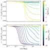 |
Fig. 1. Example of the non-linear power spectrum ratio r for varying axion abundance (top panel) and axion mass (bottom panel). We use axion mass max = 10−26 eV in the top panel, and axion abundance fax = 0.5 in the bottom panel. The data in this figure was generated using the trained axion emulator described in this paper. |
3.1. Testing the COLA setup
Hundreds of simulations are required to generate a training data-set that probes the effect of the axion mass and abundance, and the cosmological parameters. For this reason, we look to establish an optimal simulation setup that is both cost-efficient and accurate. To do this, we run a pair of ΛCDM and mixed dark matter simulations for a fiducial set of cosmological and simulation parameters to find the power spectrum ratio. By generating a new pair of simulations with one of the simulation parameters altered, and looking at the relative difference between this and the fiducial simulation run, we can study the effect of each individual parameter on the power spectrum ratio.
We tested the number of time steps, the number of grids (which is set to be equal to the number of particles) and the box size, and plot the result in Fig. 2. This test was carried out using our fiducial cosmology, but we have also performed tests to check that we have the same qualitative behavior for other cosmologies (i.e. for a few different axion masses and fractions). Our fiducial simulation setup uses 30 time steps, 640 mesh grid points and has a box size of 350 Mpc/h. We find that as long as the number of time steps is greater than ∼20, we already have sub-percent convergence. Perturbing the other parameters yields a ∼0.5% difference in the power spectrum ratio. For this reason, we run all our simulations using the fiducial setup. Initial conditions are created using 2LPT at a starting redshift of z = 30.
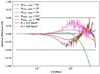 |
Fig. 2. Tests of how the power spectrum ratio, r, changes with varying simulation parameters: box size, number of time steps and grid size (force resolution). A control simulation with parameters Ntime steps = 30, Nmesh − size = 640, and B = 350 Mpc/h was used. |
We also test the COLA method itself by comparing its results with what is found when evolving the initial power spectrum with RAMSES. By comparing our approach with RAMSES, we are able to investigate the underlying error of the COLA method. The power spectrum and power spectrum ratio from both COLA and RAMSES, along with the relative difference between them, are plotted in Fig. 3. Computing the power spectrum with COLA, we find that we induce a relative difference of up to ∼60% when compared to RAMSES. At the same time, computing the power spectrum ratio, we find that we induce a relative difference of only ∼1% on small scales.
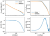 |
Fig. 3. Comparison of the power spectrum ratio, r, as calculated with COLA to what is found with RAMSES. The top left panel shows the raw power spectrum found using COLA and RAMSES, while the bottom left panel shows the relative difference between the two. The top right panel shows the ratio between the power spectrum from ΛCDM and axions, and the bottom right panel shows the relative difference of these. |
Importantly, both the differences with respect to RAMSES and with respect to simulation settings are in the regime k ≳ 1 h/Mpc where baryonic effects on the matter power spectrum are expected to be sizable (typically much larger than the differences we see here). Since we must marginalize over baryonic parameters when doing a likelihood analysis, we do not expect these ≲1% errors to play a big role if the emulator is used to extract parameter constraints (unless very strong priors on baryonic physics are assumed). In any case, these errors can easily be incorporated in a likelihood analysis as a theoretical error (see, e.g., Euclid Collaboration: Koyama et al. 2025). A more important, but currently unknown, source of error is the error of our emulator with respect to the “truth”, i.e. high resolution simulations with full axion physics. We would naively expect this to be the dominant source of error, but this remains to be checked in the future once more large-volume simulations of axions become available.
3.2. Constructing the Latin hypercube
As previously mentioned, by emulating the power spectrum ratio, we factored out some of the cosmological parameters. It is therefore important to distinguish between which parameters still have an effect on the power spectrum ratio, in order to determine what parameters need to be included in the emulation. To accomplish this, we follow a similar procedure to the previous section, where we define a fiducial set of cosmological parameters, and perturb a single parameter to explore its effect.
Fig. 4 displays the effect of Ωb, ΩDM, As, ns, h, and ΩMν on the power spectrum ratio, where we have used the fiducial parameters
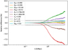 |
Fig. 4. Variation of the power spectrum ratio, r, as function of cosmological parameters. The dashed line indicates a relative difference of 1%. Only As and Ωm have significant (≳1%) deviations. An axion abundance of fax = 0.2 and axion mass of max = 10−24 eV was used. |
We find that most of the parameters are almost completely factored out, and only contribute ≲1% on small scales; however, As and Ωm still exhibit a significant contribution to the power spectrum ratio. Thus, we include this in the emulation. Furthermore, by ignoring massive neutrinos, which speed up simulations by a factor ∼2, we only induce an error of only ∼1% on small scales, which is too small to be resolved by COLA due to its intrinsic small scale error. However, the effect of all the ignored parameters is still induced implicitly since Pax = rPΛCDM and the latter factor carries parameter dependencies.
The range of the included cosmological parameters were determined by expanding the parameter range used in EUCLIDEMULATOR2 (Euclid Collaboration: Knabenhans et al. 2021). We choose to exclude some of the highest redshift results from our COLA setup, leaving us with 28 data points linearly spaced in 1/(1 + z) between z = 6.75 and z = 0. The axion abundance is probed between 1 and 0.001, as we only want to look at mixed dark matter models. For the axion mass, we go from 10−28 eV, where the axion particles behave more similarly to dark energy (Hlozek et al. 2015), to 10−22 eV, where we stop seeing the effect of the axions given our simulation setup. Thus, the final parameter space we end up with is given by:
![Mathematical equation: $$ \begin{aligned} \log _{10}{m_{\rm ax}/\mathrm{eV}}&\in [-28, -22], \\ f_{\rm ax}&\in [0.001, 1], \\ \log _{10}A_s&\in [-9, -8.52], \\ \Omega _{\rm DM}&\in [0.2, 0.4], \\ z&\in [0, 6.75], \end{aligned} $$](/articles/aa/full_html/2025/10/aa54621-25/aa54621-25-eq28.gif)
where ΩCDM = ΩDM(1 − fax) (i.e. for ΛCDM ΩDM ≡ ΩCDM).
We employed a simple wrapping scheme when creating the Latin hypercube sampling to ensure that our emulator has a sufficient amount of samples at the edges of the max and fax parameter space. In short, we sample values slightly beyond the limits of our desired sampling, and wrap the values beyond these limits back to the edges, as given above. We use the following expanded sample limits
![Mathematical equation: $$ \begin{aligned} \log _{10} m_{\rm ax}/\mathrm{eV}&\in [-28.5, -21.5], \\ f_{\rm ax}&\in [-0.1, 1.1]. \end{aligned} $$](/articles/aa/full_html/2025/10/aa54621-25/aa54621-25-eq29.gif)
Using 200 data points, we end up with the Latin hypercube sampling shown in Fig. 5. Both max and As have been sampled logarithmically.
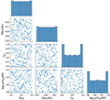 |
Fig. 5. Distribution of samples in our Latin hypercube. We increased the sample density at some of the edges in order to improve the performance of the emulator in these regions. |
3.3. The final setup
In the final COLA simulation setup, we use a box size of 350 Mpc/h, which gives us a force resolution of ∼0.5 Mpc/h and a range from k = 0.03 h/Mpc to k = 5.7 h/Mpc. The simulations run from initial redshift zini = 30 for 30 time steps. We use baryon density Ωb = 0.049, Hubble parameter h = 0.6711 and spectral index ns = 0.966. Neutrinos are ignored.
To increase the range and accuracy of the emulator in the low-k regime, we inject 256 data points from k = 10−3 h/Mpc to k = 0.02 h/Mpc using AXIONCAMB, which is sensible since this regime is linear even at redshift z = 0. Since the power spectrum with axions always tends to a ΛCDM power spectrum at low k, we get a plateau at 1 for  when we inject linear values. This helps stabilize the emulator during training.
4. Emulator
4.1. Network architecture and training
We employ a simple Feed Forward Neural Network architecture with 2 hidden layers, the first with 128 nodes and the second with 64 nodes. The input layer accepts 6 parameters (ΩDM, log10As, fax, log10max, z and k), and outputs a single value: the prediction for the power spectrum ratio for the given input values. We find that using the Gaussian Error Linear Unit (GELU) as activation functions and using the L1LOSS function to calculate the loss is sufficient. We train with learning rate γ = 0.01, weight decay set to β = 5 ⋅ 10−6 and use the Adam optimizer. Training is stopped once there is no significant improvement in the loss for 30 epochs.
The data set used for training is sampled using the LHS shown in Fig. 5, where each point is a combination of parameters that we use to calculate the power spectrum ratio. In the end, this data set contains approximately 1.9 ⋅ 106 data points. Depending on the chosen batch size, the training took between ∼15 CPU minutes and ∼3 CPU hours to train. After training, the look-up for one set of 256 Pax(k)/P(k) values takes about ∼0.05 s, which is a speed-up of a factor ∼4500 from running the N-body simulation setup to produce the same result, which takes∼4 minutes.
4.2. Emulator performance
We test the accuracy of the emulator by comparing the emulator’s prediction with the results from simulations, using the data-set used during training, and an independent data-set that the network has not been trained on. This comparison is shown in Fig. 6, where the top panel compares the training data-set and the bottom panel compares the test data-set over k for 8 different combinations of the cosmological parameters, with the error measured in squared difference:
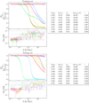 |
Fig. 6. Emulator’s performance on the training data-set (top) and test-set (bottom). The top panel shows the emulators prediction compared to the data from the simulations, and the bottom panel shows the squared error between the two. Solid lines indicate the prediction of the emulator, while dots indicate the data from simulations, with each color specifying a different set of cosmological parameters. |
 (25)
(25)
While the error varies between samples, we find that the overall error lies below 10−2. In some cases, we find a jump in error above 10−2, which may be explained by a slight misalignment between the AXIONCAMB data and the data from COLA. This may give rise to a slightly higher error in the emulator, as these transitions get smoothed over during training. Another possible source could be noise in the power spectrum boost calculated by COLA.
To test the emulator’s performance for different cosmological parameters, we calculate the mean squared error between the COLA simulations and the emulator’s prediction for each data-point in Fig. 5. The result is shown in Fig. 7. Notably, for combinations of small axion abundance and axion mass, there is an increase error, which may be due to fast changes in the power spectrum boost, caused by the strong suppression of low mass axion cosmologies.
 |
Fig. 7. Mean squared error between the emulator and COLA at each point in the Latin hypercube sampling shown in Figure 5. We find a peak error of 10−2 for combinations of small axion abundances and small axion masses. |
Additionally, we test the emulator’s ability to generate extrapolated features beyond the trained parameter-space. In Fig. 8 we demonstrate how the emulator performs on untrained values of max and fax, and compare to the prediction from COLA simulations. We find that the emulator works well in the upper limits of fax, that is fax ∼ 1, and in the chosen lower limits of max, when max ∼ 10−28 eV. In these cases, the emulator successfully predicts increased suppression for higher values of fax and suppression on larger scales for smaller max. In the lower limits of fax, we find that the emulator correctly predicts decreased suppression of power, while in the upper limit of max the emulator encounters some discrepancies, as it predicts an increase in power of ∼1%.
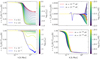 |
Fig. 8. Emulator’s performance close to and outside the parameter-space edges. The dashed lines indicate the power spectrum ratio calculated using COLA. Comparing these results to that of the emulator, it is apparent that the emulator works well close to and just outside the parameter-space edges. |
5. Comparison
We compare the power spectrum ratio predicted by the emulator with the linear prediction from AXIONCAMB, along with the standard non-linear prescription of HMCODE4 and AXIONHMCODE (Vogt et al. 2023). This comparison is shown in Fig. 9, where the top 3 × 3 panels make the comparison for small axion abundances, and the bottom 3 × 3 panels does so for larger abundances. Since HMCODE considers CDM evolution and modified initial conditions, it should, in principle, provide the best match to our simulations, which also evolve pure CDM. However, because HMCODE is calibrated to ΛCDM, it is not immediately clear how closely our simulations will follow its predictions. Meanwhile, AXIONHMCODE improves on HMCODE by including relevant axion physics, such as the impact of a cored density profile, in order to capture wave-like effects. Notably, HMCODE does not explicitly model axion physics beyond using the axion linear power spectrum, so it is only expected a priori to be accurate for very small axion fractions. Due to restrictions in AXIONHMCODE, our comparison is limited to certain combinations of max and fax.
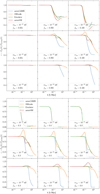 |
Fig. 9. Comparison of the power spectrum ratio from our emulator to that of naive HMCODE within CAMB, AXIONCAMB (the linear prediction) and AXIONHMCODE (a modification of HMCODE including axion physics). We were unable to run AXIONHMCODE for certain parameters choices (typically for large fax). |
In general, we find that the prediction from the emulator agrees with AXIONHMCODE and HMCODE. However, each approach predict a slightly different degree of suppression and enhancement to the power spectrum on scales smaller than the Jeans scale. For example, HMCODE predicts an enhancement to the power spectrum of up to ∼30% for axion masses around 10−23 eV. On the other hand, AXIONHMCODE predicts significant enhancements when max ∼ 10−23 eV and the axion abundance fax ≳ 0.1. Both HMCODE and AXIONHMCODE also predict a spoon shape in the power spectrum ratio on top of the suppression. Since AXIONCAMB only considers linear perturbations, it is not able to replicate this feature. This spoon shape can also be found when computing the ratio of power-spectra of massive neutrinos to ΛCDM, using either simulations (Brandbyge et al. 2008) or halo-models (Hannestad et al. 2020). The emulator does not predict any enhancements or significant spoon-shape. We note that, at present, there is no definite way to determine which model offers the most reliable baseline in the non-linear regime. Ultimately, only high-resolution simulations that consistently include axion physics will be able to clarify which features, such as enhancements and spoon shapes, are physical and which arise from model-specific assumptions.
In the work done by Vogt et al. (2023), the enhancements to the power spectrum are explained by the transition between the one- and two-halo terms overlapping with the soliton core in the halos, which dominates at that scale for axions with mass ∼10−22 eV. Similar enhancements have also been observed in simulations Nori et al. (2019). We find that enhancements can also be found when using HMCODE to calculate the power spectrum, but to a higher degree. This discrepancy likely arises from the fact that HMCODE is fitted to ΛCDM, and thus does not consider soliton cores in the 1-halo term. Fig. 11, which shows the 1- and 2-halo terms, highlights how the enhancements arise in the transition region.
Given the resolution used in this paper, we are not able to resolve the inner parts of the halos, where the halo profiles deviates from ΛCDM and instead take the form of a soliton core (Vogt et al. 2023) and thus are unable to reproduce any enhancements to the power spectrum. At the same time, we do not expect to see a soliton core within the halos as a result of the lack of the quantum pressure in the simulations. This means that, as seen in Fig. 10, our simulations mainly predict NFW profiles even for very large axion fractions.
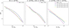 |
Fig. 10. Calculated and fitted theoretical halo profiles at redshift z = 0 for different combinations of max and fax, binned to three mass ranges. |
The halo mass function in a fuzzy DM cosmology is affected by a cutoff for small mass halos (Kulkarni & Ostriker 2022). Most studies have found that at redshift z = 0, axions with mass 10−22 eV will result in a cutoff in the halo mass function approximately between 108 M⊙ − 109 M⊙ (Marsh & Silk 2014; Bozek et al. 2015; Du et al. 2017). Given the resolution used in this study, we do not have the power to resolve halos down to this mass. For smaller axion masses, Du et al. (2017) found that the cutoff happened at increasingly higher masses, going as far as to max = 10−24 eV, where they found a cutoff roughly around ∼1012 M⊙. For even lower masses, one would expect the cutoff to happen at even higher masses, which we are able to resolve given our simulation setup. As seen in Fig. 12, while we are able to predict some suppression of the halo mass function with our approach, we are not able to reproduce the cutoff seen in the mentioned studies. Within the resolved mass range, we find that the halo mass function is reduced to the Sheth-Tormen approximation for large axion masses (∼10−22 eV), and for the most massive halos.
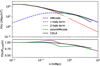 |
Fig. 11. Calculated one- and two-halo terms together with the boost for a cosmology with max = 10−25 eV and fax = 0.1. We see that the differences between HMCODE, AXIONHMCODE and the emulator mainly comes from the transition region between the two regimes. |
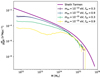 |
Fig. 12. Theoretical and calculated halo mass function for different combinations of max and fax at redshift z = 0. |
6. Conclusion
In this paper, we follow the approach of simulating a mixed axion and CDM cosmology using an approximate N-body simulation, known as the COLA method, where the axion physics come into play only through the initial conditions. Although this approach is much faster than simulating the axions by solving the Schrödinger-Poisson equations, it suffers from a lack of resolution on small scales, due to the approximative nature of the simulations, and lacks the quantum pressure associated with the axions. Some of the inaccuracies that come with a lack of resolution can be factored out by looking at the ratio between the power spectrum with axions to that of ΛCDM. This also factors out some of the dependency on the cosmological parameters.
Using this approach, we create a data-set which is used to train an emulator which predicts the boost to the power spectrum. The emulator takes six input parameters: the mass of the axion max, the axion abundance fax, As, ΩDM, redshift z, and the wave number k. We find that this emulator is in general agreement with AXIONHMCODE, which is a halo-based approach to calculate the matter power spectrum and includes the relevant axion physics. Compared to this approach, the emulator successfully predicts the suppression to the power spectrum, but fail to reproduce enhancements or a spoon-like shape seen in AXIONHMCODE. Compared to HMCODE on the other hand, a code that is fitted to ΛCDM and does not have any axion physics included, the fit is much worse. Some of the discrepancy here is probably produced by the way the transition between the 1- and 2-halo terms is modeled.
To determine the true accuracy of our method, a proper comparison to full axion simulations is required. However, such simulations are very expensive (especially for large box sizes) and were not publicly available at the present time. We hope to do this in the future. Once this is done, it will give us an estimate of the true error of our emulator, and this theoretical error can be easily incorporated into weak-lensing likelihoods (as was done in Euclid Collaboration: Koyama et al. 2025) to prevent biases in parameter constraints.
Since our approach simulates the axion particles purely as standard CDM particles, certain features may be hard toreproduce. The quantum pressure of the axions alter the halo profiles, leading to a soliton core. This is a feature that we do not expect to replicate since we do not have the quantum pressure in our simulations, and rather find that the profiles follow an NFW profile. In a mixed dark matter cosmology, the number of low-mass halos are greatly suppressed, resulting in a cutoff in the halo mass function. We do not have the resolution to fully resolve these halos. Nevertheless, we do see some effect of the axions as lighter axion masses shows signs of increasing suppression in the halo mass function.
The total cost of our emulator, including simulations and training, was around 2000 CPU hours. Given its speed and minimal computational requirements, our emulator shows promise as a powerful tool for inferring the axion mass and abundance from matter power spectrum observations. By combining our emulator with an emulator for ΛCDM one can quickly predict the power spectrum for mixed dark matter, and significantly reduce the computational load associated with running inference approaches such as MCMC samplings.
Data availability
The code and trained emulator are available on GitHub: https://github.com/frdennis/Axion-Emulator
Acknowledgments
We thank David Alonso for useful discussion and Cheng-Zong Ruan for sharing codes used for the emulation. We also thank David Marsh, Kier Rogers and Abdolali Banihashemi for sharing insightful ideas and providing valuable feedback.
References
- Albert, A., Anderson, B., Bechtol, K., et al. 2017, ApJ, 834, 110 [Google Scholar]
- Angulo, R. E., Zennaro, M., Contreras, S., et al. 2021, MNRAS, 507, 5869 [NASA ADS] [CrossRef] [Google Scholar]
- Aricò, G., Angulo, R. E., Contreras, S., et al. 2021, MNRAS, 506, 4070 [CrossRef] [Google Scholar]
- Armengaud, E., Palanque-Delabrouille, N., Yèche, C., Marsh, D. J. E., & Baur, J. 2017, MNRAS, 471, 4606 [NASA ADS] [CrossRef] [Google Scholar]
- Arnold, C., & Li, B. 2019, MNRAS, 490, 2507 [NASA ADS] [CrossRef] [Google Scholar]
- Arvanitaki, A., Dimopoulos, S., Dubovsky, S., Kaloper, N., & March-Russell, J. 2010, Phys. Rev. D, 81, 123530 [NASA ADS] [CrossRef] [Google Scholar]
- Bennett, C. L., Larson, D., Weiland, J. L., et al. 2013, ApJS, 208, 20 [Google Scholar]
- Blake, C., Kazin, E. A., Beutler, F., et al. 2011, MNRAS, 418, 1707 [NASA ADS] [CrossRef] [Google Scholar]
- Bozek, B., Marsh, D. J. E., Silk, J., & Wyse, R. F. G. 2015, MNRAS, 450, 209 [NASA ADS] [CrossRef] [Google Scholar]
- Brandbyge, J., Hannestad, S., Haugbølle, T., & Thomsen, B. 2008, JCAP, 2008, 020 [CrossRef] [Google Scholar]
- Buonaura, A. 2017, Proc. Sci., DIS2017, 079 [Google Scholar]
- Chisari, N. E., Richardson, M. L. A., Devriendt, J., et al. 2018, MNRAS, 480, 3962 [Google Scholar]
- Clowe, D., Bradač, M., Gonzalez, A. H., et al. 2006, ApJ, 648, L109 [NASA ADS] [CrossRef] [Google Scholar]
- Danninger, M. 2017, J. Phys. Conf. Ser., 888, 012039 [Google Scholar]
- Dark Energy Survey Collaboration (Abbott, T., et al.) 2016, MNRAS, 460, 1270 [Google Scholar]
- Das, S., Louis, T., Nolta, M. R., et al. 2014, JCAP, 2014, 014 [Google Scholar]
- Dawson, K. S., Schlegel, D. J., Ahn, C. P., et al. 2012, AJ, 145, 10 [Google Scholar]
- de Blok, W. J. G. 2009, Adv. Astron., 2010, 789293 [Google Scholar]
- de Jong, J. T. A., Verdoes Kleijn, G. A., Kuijken, K. H., & Valentijn, E. A. 2013, Exp. Astron., 35, 25 [Google Scholar]
- DESI Collaboration (Aghamousa, A., et al.) 2016, ArXiv e-prints [arXiv:1611.00036] [Google Scholar]
- Dome, T., May, S., Laguë, A., et al. 2024, ArXiv e-prints [arXiv:2409.11469] [Google Scholar]
- Du, X., Behrens, C., & Niemeyer, J. C. 2017, MNRAS, 465, 941 [NASA ADS] [CrossRef] [Google Scholar]
- Euclid Collaboration (Blanchard, A., et al.) 2020, A&A, 642, A191 [NASA ADS] [CrossRef] [EDP Sciences] [Google Scholar]
- Euclid Collaboration (Knabenhans, M., et al.) 2021, MNRAS, 505, 2840 [NASA ADS] [CrossRef] [Google Scholar]
- Euclid Collaboration (Koyama, K., et al.) 2025, A&A, 698, A233 [Google Scholar]
- Farren, G. S., Grin, D., Jaffe, A. H., Hložek, R., & Marsh, D. J. 2022, Phys. Rev. D, 105, 063513 [Google Scholar]
- Fidler, C., Tram, T., Rampf, C., et al. 2017, JCAP, 06, 043 [Google Scholar]
- Grin, D., Marsh, D. J. E., & Hlozek, R. 2022, Astrophysics Source Code Library [record ascl:2203.026] [Google Scholar]
- Hannestad, S., Upadhye, A., & Wong, Y. Y. Y. 2020, JCAP, 2020, 062 [CrossRef] [Google Scholar]
- Heitmann, K., Lawrence, E., Kwan, J., Habib, S., & Higdon, D. 2013, ApJ, 780, 111 [NASA ADS] [CrossRef] [Google Scholar]
- Heymans, C., Grocutt, E., Heavens, A., et al. 2013, MNRAS, 432, 2433 [Google Scholar]
- Hlozek, R., Grin, D., Marsh, D. J., & Ferreira, P. G. 2015, Phys. Rev. D, 91, 103512 [NASA ADS] [CrossRef] [Google Scholar]
- Hložek, R., Marsh, D. J., Grin, D., et al. 2017, Phys. Rev. D, 95, 123511 [Google Scholar]
- Huang, H.-J., Eifler, T., Mandelbaum, R., & Dodelson, S. 2019, MNRAS, 488, 1652 [NASA ADS] [CrossRef] [Google Scholar]
- Iršič, V., Viel, M., Haehnelt, M. G., Bolton, J. S., & Becker, G. D. 2017, Phys. Rev. Lett., 119, 031302 [CrossRef] [Google Scholar]
- Keisler, R., Reichardt, C. L., Aird, K. A., et al. 2011, ApJ, 743, 28 [Google Scholar]
- Klypin, A., Kravtsov, A. V., Valenzuela, O., & Prada, F. 1999, ApJ, 522, 82 [Google Scholar]
- Knabenhans, M., Stadel, J., Marelli, S., et al. 2019, MNRAS, 484, 5509 [Google Scholar]
- Knabenhans, M., Stadel, J., Potter, D., et al. 2021, MNRAS, 505, 2840 [NASA ADS] [CrossRef] [Google Scholar]
- Kobayashi, T., Murgia, R., De Simone, A., Iršič, V., & Viel, M. 2017, Phys. Rev. D, 96, 123514 [NASA ADS] [CrossRef] [Google Scholar]
- Kulkarni, M., & Ostriker, J. P. 2022, MNRAS, 510, 1425 [Google Scholar]
- Laguë, A., Bond, J., Hložek, R., et al. 2022, JCAP, 2022, 049 [CrossRef] [Google Scholar]
- Lewis, A., Challinor, A., & Lasenby, A. 2000, ApJ, 538, 473 [Google Scholar]
- López, S., D’Odorico, V., Ellison, S. L., et al. 2016, A&A, 594, A91 [NASA ADS] [CrossRef] [EDP Sciences] [Google Scholar]
- Macciò, A. V., Paduroiu, S., Anderhalden, D., Schneider, A., & Moore, B. 2012, MNRAS, 424, 1105 [CrossRef] [Google Scholar]
- Marsh, D. J. E. 2016, Phys. Rep., 643, 1 [NASA ADS] [CrossRef] [Google Scholar]
- Marsh, D. J. E., & Silk, J. 2014, MNRAS, 437, 2652 [NASA ADS] [CrossRef] [Google Scholar]
- Mateo, M. 1998, ARA&A, 36, 435 [NASA ADS] [CrossRef] [Google Scholar]
- May, S., & Springel, V. 2021, MNRAS, 506, 2603 [NASA ADS] [CrossRef] [Google Scholar]
- May, S., & Springel, V. 2023, MNRAS, 524, 4256 [NASA ADS] [CrossRef] [Google Scholar]
- Mina, M., Mota, D. F., & Winther, H. A. 2020, A&A, 641, A107 [EDP Sciences] [Google Scholar]
- Moore, B., Ghigna, S., Governato, F., et al. 1999, ApJ, 524, L19 [Google Scholar]
- Navarro, J. F., Frenk, C. S., & White, S. D. M. 1996, ApJ, 462, 563 [Google Scholar]
- Nishimichi, T., Takada, M., Takahashi, R., et al. 2019, ApJ, 884, 29 [NASA ADS] [CrossRef] [Google Scholar]
- Nori, M., & Baldi, M. 2018, MNRAS, 478, 3935 [Google Scholar]
- Nori, M., Murgia, R., Iršič, V., Baldi, M., & Viel, M. 2019, MNRAS, 482, 3227 [NASA ADS] [CrossRef] [Google Scholar]
- Oh, S.-H., de Blok, W. J. G., Brinks, E., Walter, F., & Kennicutt, R. C. 2011, AJ, 141, 193 [NASA ADS] [CrossRef] [Google Scholar]
- Pawlowski, M. S., Famaey, B., Merritt, D., & Kroupa, P. 2015, ApJ, 815, 19 [NASA ADS] [CrossRef] [Google Scholar]
- Persic, M., Salucci, P., & Stel, F. 1996, MNRAS, 281, 27 [Google Scholar]
- Philcox, O. H., & Ivanov, M. M. 2022, Phys. Rev. D, 105, 043517 [CrossRef] [Google Scholar]
- Planck Collaboration I. 2014, A&A, 571, A1 [NASA ADS] [CrossRef] [EDP Sciences] [Google Scholar]
- Planck Collaboration XV. 2014, A&A, 571, A15 [NASA ADS] [CrossRef] [EDP Sciences] [Google Scholar]
- Planck Collaboration XIII. 2016, A&A, 594, A13 [NASA ADS] [CrossRef] [EDP Sciences] [Google Scholar]
- Planck Collaboration XV. 2016, A&A, 594, A15 [NASA ADS] [CrossRef] [EDP Sciences] [Google Scholar]
- Rogers, K. K., & Peiris, H. V. 2021, Phys. Rev. Lett., 126, 071302 [NASA ADS] [CrossRef] [Google Scholar]
- Rogers, K. K., Hložek, R., Laguë, A., et al. 2023, JCAP, 2023, 023 [CrossRef] [Google Scholar]
- Rubin, V. C., Ford, W. K., & Thonnard, N. 1980, ApJ, 238, 471 [NASA ADS] [CrossRef] [Google Scholar]
- Sawala, T., Frenk, C. S., Fattahi, A., et al. 2014, ArXiv e-prints [arXiv:1412.2748] [Google Scholar]
- Schive, H.-Y., Chiueh, T., & Broadhurst, T. 2014, Nat. Phys., 10, 496 [NASA ADS] [CrossRef] [Google Scholar]
- Schive, H.-Y., Chiueh, T., Broadhurst, T., & Huang, K.-W. 2016, ApJ, 818, 89 [NASA ADS] [CrossRef] [Google Scholar]
- Schive, H.-Y., ZuHone, J. A., Goldbaum, N. J., et al. 2018, MNRAS, 481, 4815 [NASA ADS] [CrossRef] [Google Scholar]
- Schwabe, B., Gosenca, M., Behrens, C., Niemeyer, J. C., & Easther, R. 2020, Phys. Rev. D, 102, 083518 [Google Scholar]
- Seljak, U. 2000, MNRAS, 318, 203 [Google Scholar]
- Sheth, R. K., Mo, H. J., & Tormen, G. 2001, MNRAS, 323, 1 [NASA ADS] [CrossRef] [Google Scholar]
- Spergel, D., Gehrels, N., Baltay, C., et al. 2015, ArXiv e-prints [arXiv:1503.03757] [Google Scholar]
- Tassev, S., Zaldarriaga, M., & Eisenstein, D. J. 2013, JCAP, 2013, 036 [Google Scholar]
- The LSST Dark Energy Science Collaboration (Mandelbaum, R., et al.) 2021, ArXiv e-prints [arXiv:1809.01669] [Google Scholar]
- Veltmaat, J., & Niemeyer, J. C. 2016, Phys. Rev. D, 94, 123523 [Google Scholar]
- Vogt, S. M., Marsh, D. J., & Laguë, A. 2023, Phys. Rev. D, 107, 063526 [NASA ADS] [CrossRef] [Google Scholar]
- Walker, M. G., & Peñarrubia, J. 2011, ApJ, 742, 20 [CrossRef] [Google Scholar]
- Winther, H. A., Koyama, K., Manera, M., Wright, B. S., & Zhao, G.-B. 2017, JCAP, 08, 006 [CrossRef] [Google Scholar]
- Wittman, D. M., Tyson, J. A., Dell’Antonio, I. P., et al. 2002, Proc. SPIE, 4836, 73 [Google Scholar]
- Woo, T.-P., & Chiueh, T. 2009, ApJ, 697, 850 [NASA ADS] [CrossRef] [Google Scholar]
- Zwicky, F. 1937, ApJ, 86, 217 [NASA ADS] [CrossRef] [Google Scholar]
All Figures
|
Fig. 1. Example of the non-linear power spectrum ratio r for varying axion abundance (top panel) and axion mass (bottom panel). We use axion mass max = 10−26 eV in the top panel, and axion abundance fax = 0.5 in the bottom panel. The data in this figure was generated using the trained axion emulator described in this paper. |
| In the text | |
|
Fig. 2. Tests of how the power spectrum ratio, r, changes with varying simulation parameters: box size, number of time steps and grid size (force resolution). A control simulation with parameters Ntime steps = 30, Nmesh − size = 640, and B = 350 Mpc/h was used. |
| In the text | |
|
Fig. 3. Comparison of the power spectrum ratio, r, as calculated with COLA to what is found with RAMSES. The top left panel shows the raw power spectrum found using COLA and RAMSES, while the bottom left panel shows the relative difference between the two. The top right panel shows the ratio between the power spectrum from ΛCDM and axions, and the bottom right panel shows the relative difference of these. |
| In the text | |
|
Fig. 4. Variation of the power spectrum ratio, r, as function of cosmological parameters. The dashed line indicates a relative difference of 1%. Only As and Ωm have significant (≳1%) deviations. An axion abundance of fax = 0.2 and axion mass of max = 10−24 eV was used. |
| In the text | |
|
Fig. 5. Distribution of samples in our Latin hypercube. We increased the sample density at some of the edges in order to improve the performance of the emulator in these regions. |
| In the text | |
|
Fig. 6. Emulator’s performance on the training data-set (top) and test-set (bottom). The top panel shows the emulators prediction compared to the data from the simulations, and the bottom panel shows the squared error between the two. Solid lines indicate the prediction of the emulator, while dots indicate the data from simulations, with each color specifying a different set of cosmological parameters. |
| In the text | |
|
Fig. 7. Mean squared error between the emulator and COLA at each point in the Latin hypercube sampling shown in Figure 5. We find a peak error of 10−2 for combinations of small axion abundances and small axion masses. |
| In the text | |
|
Fig. 8. Emulator’s performance close to and outside the parameter-space edges. The dashed lines indicate the power spectrum ratio calculated using COLA. Comparing these results to that of the emulator, it is apparent that the emulator works well close to and just outside the parameter-space edges. |
| In the text | |
|
Fig. 9. Comparison of the power spectrum ratio from our emulator to that of naive HMCODE within CAMB, AXIONCAMB (the linear prediction) and AXIONHMCODE (a modification of HMCODE including axion physics). We were unable to run AXIONHMCODE for certain parameters choices (typically for large fax). |
| In the text | |
|
Fig. 10. Calculated and fitted theoretical halo profiles at redshift z = 0 for different combinations of max and fax, binned to three mass ranges. |
| In the text | |
|
Fig. 11. Calculated one- and two-halo terms together with the boost for a cosmology with max = 10−25 eV and fax = 0.1. We see that the differences between HMCODE, AXIONHMCODE and the emulator mainly comes from the transition region between the two regimes. |
| In the text | |
|
Fig. 12. Theoretical and calculated halo mass function for different combinations of max and fax at redshift z = 0. |
| In the text | |
Current usage metrics show cumulative count of Article Views (full-text article views including HTML views, PDF and ePub downloads, according to the available data) and Abstracts Views on Vision4Press platform.
Data correspond to usage on the plateform after 2015. The current usage metrics is available 48-96 hours after online publication and is updated daily on week days.
Initial download of the metrics may take a while.