| Issue |
A&A
Volume 702, October 2025
|
|
|---|---|---|
| Article Number | A125 | |
| Number of page(s) | 12 | |
| Section | Stellar structure and evolution | |
| DOI | https://doi.org/10.1051/0004-6361/202554721 | |
| Published online | 20 October 2025 | |
Constraining the TeV gamma-ray emission of SN 2024bch, a possible type IIn-L from a red supergiant progenitor
Multiwavelength observations and analysis of the progenitor
1
Department of Physics, Tokai University, 4-1-1, Kita-Kaname, Hiratsuka, Kanagawa 259-1292, Japan
2
Institute for Cosmic Ray Research, University of Tokyo, 5-1-5, Kashiwa-no-ha, Kashiwa, Chiba 277-8582, Japan
3
INFN and Università degli Studi di Siena, Dipartimento di Scienze Fisiche, della Terra e dell’Ambiente (DSFTA), Sezione di Fisica, Via Roma 56, 53100 Siena, Italy
4
Université Paris-Saclay, Université Paris Cité, CEA, CNRS, AIM, F-91191 Gif-sur-Yvette Cedex, France
5
FSLAC IRL 2009, CNRS/IAC, La Laguna, Tenerife, Spain
6
Departament de Física Quàntica i Astrofísica, Institut de Ciències del Cosmos, Universitat de Barcelona, IEEC-UB, Martí i Franquès, 1, 08028 Barcelona, Spain
7
Instituto de Astrofísica de Andalucía-CSIC, Glorieta de la Astronomía s/n, 18008 Granada, Spain
8
Department of Astronomy, University of Geneva, Chemin d’Ecogia 16, CH-1290 Versoix, Switzerland
9
INFN Sezione di Napoli, Via Cintia, ed. G, 80126 Napoli, Italy
10
INAF – Osservatorio Astronomico di Roma, Via di Frascati 33, 00040 Monteporzio Catone, Italy
11
Max-Planck-Institut für Physik, Boltzmannstraße 8, 85748 Garching bei München, Germany
12
INFN Sezione di Padova and Università degli Studi di Padova, Via Marzolo 8, 35131 Padova, Italy
13
Instituto de Astrofísica de Canarias and Departamento de Astrofísica, Universidad de La Laguna, C. Vía Láctea, s/n, 38205 La Laguna, Santa Cruz de Tenerife, Spain
14
Univ. Savoie Mont Blanc, CNRS, Laboratoire d’Annecy de Physique des Particules – IN2P3, 74000 Annecy, France
15
Universität Hamburg, Institut für Experimentalphysik, Luruper Chaussee 149, 22761 Hamburg, Germany
16
Graduate School of Science, University of Tokyo, 7-3-1 Hongo, Bunkyo-ku, Tokyo 113-0033, Japan
17
IPARCOS-UCM, Instituto de Física de Partículas y del Cosmos, and EMFTEL Department, Universidad Complutense de Madrid, Plaza de Ciencias, 1. Ciudad Universitaria, 28040 Madrid, Spain
18
Faculty of Science and Technology, Universidad del Azuay, Cuenca, Ecuador
19
Centro Brasileiro de Pesquisas Físicas, Rua Xavier Sigaud 150, RJ, 22290-180 Rio de Janeiro, Brazil
20
CIEMAT, Avda. Complutense 40, 28040 Madrid, Spain
21
University of Geneva – Département de physique Nucléaire et corpusculaire, 24 Quai Ernest Ansernet, 1211 Genève 4, Switzerland
22
INFN Sezione di Bari and Politecnico di Bari, Via Orabona 4, 70124 Bari, Italy
23
Institut de Fisica d’Altes Energies (IFAE), The Barcelona Institute of Science and Technology, Campus UAB, 08193 Bellaterra (Barcelona), Spain
24
INAF – Osservatorio Astronomico di Brera, Via Brera 28, 20121 Milano, Italy
25
Faculty of Physics and Applied Informatics, University of Lodz, ul. Pomorska 149-153, 90-236 Lodz, Poland
26
INAF – Osservatorio di Astrofisica e Scienza dello spazio di Bologna, Via Piero Gobetti 93/3, 40129 Bologna, Italy
27
Dipartimento di Fisica e Astronomia (DIFA) Augusto Righi, Università di Bologna, via Gobetti 93/2, I-40129 Bologna, Italy
28
Lamarr Institute for Machine Learning and Artificial Intelligence, 44227 Dortmund, Germany
29
INFN Sezione di Trieste and Università degli studi di Udine, Via delle scienze 206, 33100 Udine, Italy
30
INAF – Istituto di Astrofisica e Planetologia Spaziali (IAPS), Via del Fosso del Cavaliere 100, 00133 Roma, Italy
31
Aix Marseille Univ, CNRS/IN2P3, CPPM, Marseille, France
32
University of Alcalá UAH, Departamento de Physics and Mathematics, Pza. San Diego, 28801 Alcalá de Henares, Madrid, Spain
33
INFN Sezione di Bari and Università di Bari, via Orabona 4, 70126 Bari, Italy
34
INFN Sezione di Torino, Via P. Giuria 1, 10125 Torino, Italy
35
Dipartimento di Fisica – Universitá degli Studi di Torino, Via Pietro Giuria 1, 10125 Torino, Italy
36
Palacky University Olomouc, Faculty of Science, 17. listopadu 1192/12, 771 46 Olomouc, Czech Republic
37
Dipartimento di Fisica e Chimica ‘E. Segrè’ Università degli Studi di Palermo, Via delle Scienze, 90128 Palermo, Italy
38
INFN Sezione di Catania, Via S. Sofia 64, 95123 Catania, Italy
39
IRFU, CEA, Université Paris-Saclay, Bât 141, 91191 Gif-sur-Yvette, France
40
Port d’Informació Científica, Edifici D, Carrer de l’Albareda, 08193 Bellaterrra (Cerdanyola del Vallès), Spain
41
INFN Sezione di Bari, Via Orabona 4, 70125 Bari, Italy
42
Department of Physics, TU Dortmund University, Otto-Hahn-Str. 4, 44227 Dortmund, Germany
43
University of Rijeka, Department of Physics, Radmile Matejcic 2, 51000 Rijeka, Croatia
44
Institute for Theoretical Physics and Astrophysics, Universität Würzburg, Campus Hubland Nord, Emil-Fischer-Str. 31, 97074 Würzburg, Germany
45
Department of Physics and Astronomy, University of Turku, Finland, FI-20014 University of Turku, Finland
46
Department of Physics, TU Dortmund University, Otto-Hahn-Str. 4, 44227 Dortmund, Germany
47
INFN Sezione di Roma La Sapienza, P.le Aldo Moro, 2, 00185 Rome, Italy
48
ILANCE, CNRS – University of Tokyo International Research Laboratory, University of Tokyo, 5-1-5 Kashiwa-no-Ha Kashiwa City, Chiba 277-8582, Japan
49
Physics Program, Graduate School of Advanced Science and Engineering, Hiroshima University, 1-3-1 Kagamiyama, Higashi-Hiroshima City, Hiroshima 739-8526, Japan
50
INFN Sezione di Roma Tor Vergata, Via della Ricerca Scientifica 1, 00133 Rome, Italy
51
University of Split, FESB, R. Boškovića 32, 21000 Split, Croatia
52
Department of Physics, Yamagata University, 1-4-12 Kojirakawa-machi, Yamagata-shi 990-8560, Japan
53
Institut für Theoretische Physik, Lehrstuhl IV: Plasma-Astroteilchenphysik, Ruhr-Universität Bochum, Universitätsstraße 150, 44801 Bochum, Germany
54
Sendai College, National Institute of Technology, 4-16-1 Ayashi-Chuo, Aoba-ku, Sendai city, Miyagi 989-3128, Japan
55
Josip Juraj Strossmayer University of Osijek, Department of Physics, Trg Ljudevita Gaja 6, 31000 Osijek, Croatia
56
Department of Astronomy and Space Science, Chungnam National University, Daejeon 34134, Republic of Korea
57
INFN Dipartimento di Scienze Fisiche e Chimiche – Università degli Studi dell’Aquila and Gran Sasso Science Institute, Via Vetoio 1, Viale Crispi 7, 67100 L’Aquila, Italy
58
Chiba University, 1-33, Yayoicho, Inage-ku, Chiba-shi, Chiba 263-8522, Japan
59
Kitashirakawa Oiwakecho, Sakyo Ward, Kyoto 606-8502, Japan
60
FZU – Institute of Physics of the Czech Academy of Sciences, Na Slovance 1999/2, 182 21 Praha 8, Czech Republic
61
Laboratory for High Energy Physics, École Polytechnique Fédérale, CH-1015 Lausanne, Switzerland
62
Astronomical Institute of the Czech Academy of Sciences, Bocni II 1401, 14100 Prague, Czech Republic
63
Faculty of Science, Ibaraki University, 2 Chome-1-1 Bunkyo, Mito, Ibaraki 310-0056, Japan
64
Sorbonne Université, CNRS/IN2P3, Laboratoire de Physique Nucléaire et de Hautes Energies, LPNHE, 4 place Jussieu, 75005 Paris, France
65
Graduate School of Science and Engineering, Saitama University, 255 Simo-Ohkubo, Sakura-ku, Saitama city, Saitama 338-8570, Japan
66
Institute of Particle and Nuclear Studies, KEK (High Energy Accelerator Research Organization), 1-1 Oho, Tsukuba 305-0801, Japan
67
INFN Sezione di Trieste and Università degli Studi di Trieste, Via Valerio 2 I, 34127 Trieste, Italy
68
Escuela Politécnica Superior de Jaén, Universidad de Jaén, Campus Las Lagunillas s/n, Edif. A3, 23071 Jaén, Spain
69
Saha Institute of Nuclear Physics, Sector 1, AF Block, Bidhan Nagar, Bidhannagar, Kolkata, West Bengal 700064, India
70
Institute for Nuclear Research and Nuclear Energy, Bulgarian Academy of Sciences, 72 boul. Tsarigradsko chaussee, 1784 Sofia, Bulgaria
71
Department of Physics and Astronomy, Clemson University, Kinard Lab of Physics, Clemson, SC 29634, USA
72
Institut de Fisica d’Altes Energies (IFAE), The Barcelona Institute of Science and Technology, Campus UAB, 08193 Bellaterra (Barcelona), Spain
73
Grupo de Electronica, Universidad Complutense de Madrid, Av. Complutense s/n, 28040 Madrid, Spain
74
Institute of Space Sciences (ICE, CSIC), and Institut d’Estudis Espacials de Catalunya (IEEC), and Institució Catalana de Recerca I Estudis Avançats (ICREA), Campus UAB, Carrer de Can Magrans, s/n, 08193 Bellatera, Spain
75
Department of Physics, Konan University, 8-9-1 Okamoto, Higashinada-ku Kobe 658-8501, Japan
76
School of Allied Health Sciences, Kitasato University, Sagamihara, Kanagawa 228-8555, Japan
77
RIKEN, Institute of Physical and Chemical Research, 2-1 Hirosawa, Wako, Saitama 351-0198, Japan
78
Charles University, Institute of Particle and Nuclear Physics, V Holešovičkách 2, 180 00 Prague 8, Czech Republic
79
Division of Physics and Astronomy, Graduate School of Science, Kyoto University, Sakyo-ku, Kyoto 606-8502, Japan
80
Institute for Space-Earth Environmental Research, Nagoya University, Chikusa-ku, Nagoya 464-8601, Japan
81
Kobayashi-Maskawa Institute (KMI) for the Origin of Particles and the Universe, Nagoya University, Chikusa-ku, Nagoya 464-8602, Japan
82
Graduate School of Technology, Industrial and Social Sciences, Tokushima University, 2-1 Minamijosanjima, Tokushima 770-8506, Japan
83
INFN Sezione di Pisa, Edificio C – Polo Fibonacci, Largo Bruno Pontecorvo 3, 56127 Pisa, Italy
84
Gifu University, Faculty of Engineering, 1-1 Yanagido, Gifu 501-1193, Japan
85
Department of Physical Sciences, Aoyama Gakuin University, Fuchinobe, Sagamihara, Kanagawa 252-5258, Japan
86
Macroarea di Scienze MMFFNN, Università di Roma Tor Vergata, Via della Ricerca Scientifica 1, 00133 Rome, Italy
⋆ Corresponding authors: This email address is being protected from spambots. You need JavaScript enabled to view it.
Received:
24
March
2025
Accepted:
30
July
2025
Abstract
We present very high-energy optical photometry and spectroscopic observations of SN 2024bch in the nearby galaxy NGC 3206 (∼20 Mpc). We used gamma-ray observations performed with the first Large-Sized Telescope (LST-1) of the Cherenkov Telescope Array Observatory (CTAO) and optical observations with the Liverpool Telescope (LT) combined with data from public repositories to evaluate the general properties of the event and the progenitor star. No significant emission above the LST-1 energy threshold for this observation (∼100 GeV) was detected in the direction of SN 2024bch, and we computed an integral upper limit on the photon flux of Fγ(> 100 GeV)≤3.61 × 10⁻¹² cm−2 s−1 based on six nonconsecutive nights of observations with the LST-1, between 16 and 38 days after the explosion. Employing a general model for the gamma-ray flux emission, we found an upper limit on the mass-loss-rate to wind-velocity ratio of Ṁ/uw ≤ 10−4 M⊙/ yr s/km, although gamma-gamma absorption could potentially have skewed this estimation, effectively weakening our constraint. From spectro-photometric observations we found progenitor parameters of Mpr = 11 – 20 M⊙ and Rpr = 531 ± 125 R⊙. Finally, using archival images from the Hubble Space Telescope, we constrained the luminosity of the progenitor star to log (Lpr/L⊙) ≤ 4.82 and its effective temperature to Tpr ≤ 4000 K. Our results suggest that SN 2024bch is a type IIn-L supernova that originated from a progenitor star consistent with a red supergiant. We show how the correct estimation of the mass-loss history of a supernova will play a major role in future multiwavelength observations.
Key words: supernovae: general / supernovae: individual: SN 2024bch / gamma rays: general
© The Authors 2025
 Open Access article, published by EDP Sciences, under the terms of the Creative Commons Attribution License (https://creativecommons.org/licenses/by/4.0), which permits unrestricted use, distribution, and reproduction in any medium, provided the original work is properly cited.
This article is published in open access under the Subscribe to Open model. This email address is being protected from spambots. You need JavaScript enabled to view it. to support open access publication.
1. Introduction
Core-collapse supernovae (CCSNe) are the final product of the evolution of massive stars. They are among the most energetic phenomena in our Universe and are ideal sources for multiwavelength and multi-messenger studies, as notably proven by the detection of neutrinos from SN 1987A (Bionta et al. 1987; Hirata et al. 1987). Despite the fact that many supernovae (SNe) have been extensively characterized from the radio to the X-ray band, with possible detections up to soft gamma rays (Yuan et al. 2018; Xi et al. 2020; Chen et al. 2024), the physical processes and mechanisms behind the collapse are not yet fully understood.
Supernovae can be powerful cosmic ray (CR) accelerators and are believed to produce gamma rays up to the very high-energy (VHE) band (E ≥ 100 GeV; Marcowith et al. 2018). The interaction of the fast energetic SN ejecta with a dense and slower circumstellar medium (CSM) surrounding the progenitor triggers the formation of shock waves, which give rise to thermal optical, UV, and X-ray emission. Collisionless shocks are expected to accelerate a fraction of the charged particles up to high relativistic energies via the diffusive shock acceleration mechanism (e.g., Longair 2011; Murase et al. 2011; Bell et al. 2013), leading to nonthermal emission (Chevalier & Fransson 2017). In this scenario, proton–proton interactions between the accelerated protons and the CSM may give rise to VHE gamma rays (Murase 2024). The VHE gamma-ray flux is expected to peak shortly after the explosion, when the SN ejecta encounter the innermost, densest region of the CSM, leading to an increase in proton–proton interactions (Brose et al. 2022).
However, during the first tens to hundreds of days after the explosion, the possible VHE signal is significantly attenuated by the gamma-gamma absorption resulting from the interactions of VHE gamma rays with the soft optical photons emitted by the SN photosphere (e.g., Tatischeff 2009; Bykov et al. 2018; Cristofari et al. 2022; Brose et al. 2022). However, a detailed characterization of this process is made difficult by the high number of degrees of freedom and degeneracy among the relevant parameters. Attenuation is influenced not only by the intrinsic properties of the SN itself, but also by the characteristics of the ejected material, the structure of the CSM (which is shaped by the progenitor star’s mass-loss history), and the evolution of the photosphere, as its temperature and radius determine the population of low-energy target photons.
To date, the dedicated VHE gamma-ray follow-up campaigns for different types of SNe performed by the current generation of Imaging Atmospheric Cherenkov Telescopes (IACTs) have not achieved any significant detections (Ahnen et al. 2017; Abdalla et al. 2019; Acharyya et al. 2023). Nevertheless, the quest for gamma-ray signals from CCSNe remains an important goal for current and next-generation VHE facilities. In particular, future facilities such as the Cherenkov Telescope Array Observatory (CTAO; Cherenkov Telescope Array Consortium 2019), with its foreseen improved sensitivity and wider accessible energy range, will likely be able to detect VHE counterpart of CCSNe up to ∼10 Mpc (e.g., Bošnjak et al. 2021), boosting our understanding of the physical mechanisms at work.
The standard classification scheme of SNe groups different events based on their spectral features (e.g., Filippenko 1997, and references therein). In particular, type II SNe exhibit hydrogen-rich spectra. These are the most common events and are typically associated with massive red supergiant (RSG) progenitors. Depending on the shape of their optical light curves, they were historically divided into type II-L (linear) and typeII-P (plateau) based on the relative decay rate (Barbon et al. 1979). Although several studies have found evidence that the distribution of decay rates is a continuum (e.g., Patat et al. 1994; Anderson et al. 2014; Gall et al. 2015; Sanders et al. 2015), others suggest that a bimodal distribution can be seen when focusing on the decay rates of specific time ranges. Li et al. (2011) and Faran et al. (2014) proposed a new method for discriminating between the two classes: the R-band (V-band) luminosity has to decay by 0.5 magnitudes or more between the peak of luminosity and 50 days after the explosion (t50).
A further subtype of hydrogen-rich SNe is the type IIn. They exhibit spectra dominated by strong Balmer emission lines on a blue continuum, indicating a hydrogen-rich environment possibly caused by strong mass loss before the explosion (Schlegel 1990). These lines often include a narrow component – with a full width at half maximum (FWHM) of about 100 km s−1 – from the un-shocked CSM and broader components (FWHM of several thousand km s−1) arising from the interaction between the rapidly expanding ejecta and the slow, dense CSM (e.g., Chevalier & Fransson 1994). To form a CSM sufficiently dense to allow such narrow lines to persist for a long period after the explosion, the progenitor star must undergo significant mass loss prior to the explosion. Luminous blue variable (LBV) stars are often proposed as possible direct progenitors of type IIn SNe (Kotak & Vink 2006; Trundle et al. 2008; Gal-Yam & Leonard 2009). However, RSG candidates are also a widely considered possibility (e.g., Fransson et al. 2002; Smith et al. 2009; Mackey et al. 2014) despite likely not being major contributors, given the relative rates of type IIn SNe (e.g., Cold & Hjorth 2023) and the limited mass range from which RSGs originate.
Due to the combination of high luminosity and strong CSM interactions, type IIn SNe are among the most likely CCSNe to exhibit a VHE emission component (e.g., Murase 2024). However, significant differences can exist between individual type IIn SNe due to different CSM properties, explosion parameters, and potential progenitor channels. For this reason, new subclasses have recently been suggested based on their photometric and spectroscopic evolution (Taddia et al. 2013; Habergham et al. 2014; Taddia et al. 2015). Among them, IIn-L SNe are classified based on their similarity to SN 1998S (Chugai 2001; Fassia et al. 2001). Their light curves exhibit a rapid type IIL-like decline, while their early-time spectral evolution resembles that of type IIn SNe. At later times, this evolves into a more typical IIL-like behavior, with broader lines. As in the case of SN 1998S, signatures of CSM interaction can persist at late times, indicating different episodes of mass-loss before the explosion (Pozzo et al. 2004). Overall, this behavior indicates a low-mass CSM (e.g., Smith 2017). In recent years, some SNe originally classified as type IIn have been reclassified as IIn-L under this newer definition (e.g., Faran et al. 2014; Kangas et al. 2016). Their explosion sites have been found to be metal-rich, similar to those of normal type II-L and II-P SNe, supporting the scenario of massive RSG progenitors (Taddia et al. 2015).
SN 2024bch was discovered on January 29, 2024, at 06:02:50 UTC in the barred spiral galaxy NGC 3206 (z = 0.003863; μ = 31.49 ± 0.45;  Mpc; Tully et al. 2016; Castignani et al. 2022), at coordinates RA(J2000) = 10h 21m 50.200s, Dec(J2000) = +56° 55′ 36.10″ (Wiggins 2024). It was initially classified as a type IIn due to its spectral similarity with SN 1998S at 3.5 days after the explosion (Balcon 2024). SN 2024bch has been studied extensively in the optical band and has been classified as a type II with CSM interaction (Tartaglia et al. 2024; Andrews et al. 2025). We present VHE follow-up observations of SN 2024bch made with the CTAO Large-Sized Telescope prototype (LST-1) and optical follow-up taken with the Liverpool Telescope (LT). The latter allowed us to recover one spectrum at ∼50 days after the explosion. We combined our VHE gamma-ray and optical observations to determine the general properties and the type of the event and its progenitor star. The spectrophotometric evolution in the optical band is crucial for constraining some of the parameters required to model the gamma-ray flux and reduce systematic uncertainties. This multiwavelength approach may play a significant role in correctly modeling observations with current and future IACTs.
The paper is structured as follows: We present our VHE gamma-ray and optical observations and analysis in Sects. 2 and 3, respectively. In Sect. 4 we focus on constraining the physical parameters of the SN explosion, the SN ejecta, and the progenitor star. In Sect. 5 we discuss how our results can be used to determine the class and progenitor star of SN 2024bch, while in Sect. 6 we discuss how our data may be affected by gamma-gamma absorption. Finally, we outline our conclusions in Sect. 7.
2. VHE observations and data analysis
The LST-1 is the first 23 m diameter telescope that will form the core of the upcoming northern array of the CTAO (CTAO-N; Cherenkov Telescope Array Consortium 2019). The telescope is located at the Observatorio del Roque de los Muchachos in the Canary Island of La Palma, Spain. Thanks to its large reflecting area of ∼400 m2 and a camera constituted by high-quantum efficiency photomultiplier tubes, LST-1 is optimized for observations at the lowest energy edge of the VHE band, above a few tens of GeV (Abe et al. 2023a).
We triggered target of opportunity (ToO) observations on SN 2024bch with the LST-1 starting from February 13, 2024 (MJD 60353), about two weeks after its discovery. The follow-up began with a two-week delay because the gamma-gamma attenuation is expected to be strong during the first days after the explosion (see Sect. 6). The follow-up was extended for a total of six nonconsecutive nights collecting 14.6 hours of observations between February and March 2024 in the zenith range 28°–43°. Observations were performed in the so-called wobble mode (Fomin et al. 1994) and in good atmospheric and in dark-to-low-moonlight conditions. The corresponding energy threshold is about ∼30 GeV.
We followed a source-independent standard analysis scheme for SN 2024bch gamma-ray data, as described in Abe et al. (2023b). After applying data quality cuts, based on pointing stability, level of constant night sky background and intensity of CRs, we selected 12.0 hours of good quality data. Data reduction is performed using the software package cta-lstchain v0.10.7, the standard analysis pipeline for LST-1 data (López-Coto et al. 2021; Lopez-Coto et al. 2024). From the recorded shower images, random forests trained on Monte Carlo simulations, produced at a fixed declination of +61.66° (4.73° away from the SN 2024bch position), are used to determine the parameters of the incoming primary particles, energy, direction and gammaness, a score for gamma-hadron separation. After determining the shower parameters, event selection cuts were applied and the data were processed to the final scientific level, where the response of the telescope was characterized using instrument response functions derived from Monte Carlo simulations assuming a point-like source hypothesis.
For the 1D spectral analysis we used the open-source tool Gammapy (Donath et al. 2023; Acero et al. 2024). We used one OFF region (i.e., a reflected region with respect to the ON region centered at the source position) to model and subtract the background contribution from our data, specifically the irreducible background from isotropic gamma rays and gamma-like hadronic air showers.
No significant gamma-ray excess was detected on any of the observed nights or from the full dataset. We computed upper limits (ULs) for the spectral energy distribution of SN 2024bch between 75 GeV and 10 TeV, assuming a single power law with a spectral index of Γ = −2.5 (see Sect. 4.1). The spectral energy distribution is shown in Fig. 1. Additionally, we calculated night-wise light curve ULs between 100 GeV and 10 TeV. Using the same spectral index, we also computed the integrated UL. We show our results in Fig. 2 and Table 1.
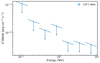 |
Fig. 1. LST-1 differential ULs obtained from SN 2024bch observations between 75 GeV and 10 TeV, estimated with three energy bins per decade and assuming a fixed spectral index of –2.5 considering the full time-range. ULs are computed with a 2σ confidence level. |
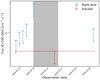 |
Fig. 2. ULs for the gamma-ray light curves of SN 2024bch, computed between 100 GeV and 10 TeV. We compare the night-wise ULs (blue) with the integrated UL, obtained by stacking all results together (red). The gray-shaded area covers the nights with strong moonlight. ULs are computed with a 2σ confidence level. |
Results of the LST-1 observations.
3. Optical observations
3.1. Light curves
We collected photometric data available in the American Association of Variable Star Observers (AAVSO) repository (Kloppenborg 2024) in four bands (B, V, R, and I). All magnitudes were converted into the relative standard photometric system and K-corrected. These light curves range between MJD 60341 and MJD 60455, covering the region around the peak and the plateau phase. The light-curve drop indicating the switch between plateau and nebular phase is only clearly visible in the R band. We inferred a time of explosion of t0 = 60337.4 ± 1.9 MJD, which is adopted as reference time throughout the paper. Furthermore, the V band peaks at tmax = 60347.3 ± 1.7 MJD. We adopted a reddening along the line of sight of EB − V = 0.049, as estimated in Andrews et al. (2025) from Na ID line measurements. The distance of the event was assumed as the average distance of NGC 3206 from redshift-independent estimates from NASA Extragalactic Database (NED)1. We find d = 17.6 ± 1.1 Mpc, corresponding to a distance modulus of μ = 31.23 ± 0.13. All photometric data used in this analysis are shown in Fig. 3, compared with the LST-1 observing nights.
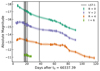 |
Fig. 3. Public photometry of SN 2024bch (filled points). We used observations in the four filters B, V, R, and I. An offset is added to the data points for a better visualization. Solid lines are the result of GP interpolation obtained with CASTOR (see the main text). The uncertainties of the interpolated lines are shown as shaded contours. The vertical solid black lines show the LST-1 observation windows. |
We used the open-access software CASTOR v2.0 (Simongini et al. 2024, 2025) to interpolate our light curves via Gaussian process (GP) regression techniques and compared them to a catalog of 150 CCSNe via chi-square test. We found this SN to be most similar to SN 2009kr (Elias-Rosa et al. 2010), SN 2013fc (Kangas et al. 2016), and SN 2008fq (Faran et al. 2014), as shown in Fig. 4. These CCSNe were all classified as type II, with linear decaying light curves and 1998S-like spectra. The interpolated V-band light curve of SN 2024bch decays by 1.05 ± 0.11 magnitudes between the peak of luminosity and t50, while the R-band light curve decays by 0.74 ± 0.10 magnitudes (see Fig. 4). According to the criteria determined by Li et al. (2011) and Faran et al. (2014), and to the statistical comparison performed with CASTOR, SN 2024bch shows a clear linear decay tens of days after the explosion, similar to a common type II-L.
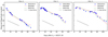 |
Fig. 4. Comparison of the BVR light curves of SN 2024bch (blue dots) with those of SN 2009kr and SN 2013fc (dashed red and green curves, respectively). The data for SN 2009kr and SN 2013fc are scaled to match SN 2024bch and interpolated over the same time interval using GP interpolation (see the main text for details). Additionally, we show a reference curve representing a decay of 1 magnitude between tmax and t50. |
3.2. Spectra
SN 2024bch was observed on a single night by the LT (Steele et al. 2004) via a ToO observation. The LT is a 2-m robotic Cassegrain reflector, located at the same site as the LST-1. Low-resolution (R = 350) spectroscopy was performed on MJD 60385.018, 47.6 days after the explosion with the SPRAT spectrograph (Piascik et al. 2014). We obtained one spectrum in the range 4000–8000 Å as shown in Fig. 5. Data were reduced using the standard LT pipeline. Our LT spectrum is complemented with ancillary low-resolution spectra collected from WISeREP (Yaron & Gal-Yam 2012). All spectra were taken between 4000 and 9000 Å in the host-galaxy reference frame and thus are not redshift-corrected. We cut every spectrum between 4000 and 8300 Å to avoid data with low signal-to-noise ratios (S/Ns), effectively removing the near-IR region of the spectrum. Figure 5 shows the temporal evolution of SN 2024bch spectra between 1 and 55 days after the explosion. The main spectral features are highlighted with vertical lines. At early times (8, 6, 4, and 3 days before the peak of maximum luminosity, MJD 60347.19, t0 + 9 days), the spectra consist of a blue, almost featureless continuum. The only discernible lines, apart from the telluric lines around 7580 Å and 6848 Å, are the Balmer lines at 6563 Å, 4861 Å, and 4341 Å, the C IV line at 5801 Å, and the N III line at 4687 Å. By mid-late times (35 and 45 days after the peak), the blue continuum has cooled. The Hα is considerably broader and stronger and has remained the most distinguishable feature along with the Hβ line, which is weaker and broader. The N III line at 4687 Å is less discernible and possibly blended with Mg I] line at 4571 Å. The C IV line at 5801 Å has been substituted by a Na ID line at 5895 Å.
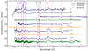 |
Fig. 5. Spectra of SN 2024bch compared with two spectra of SN 2013fc (at 17 and 51 days post-explosion) and two spectra of SN 2008fq (at 6 and 57 days post-explosion). We removed the continuum from every spectrum and normalized to order zero. We added an offset for better visualization. The main spectral features of SN 2024bch are highlighted as purple-shaded vertical bands. Telluric lines are identified as “T1” and “T2” (gray bands). The spectrum taken with LT is the second from the bottom of the SN 2024bch spectra, at 47 days post-explosion. The other spectral data for the three SNe are taken from WISeREP (Yaron & Gal-Yam 2012). |
The characteristic Hα profile appears to undergo a significant change in morphology between early and late phases. We decomposed the line into a Lorentzian and a Gaussian profile at early times (respectively for the narrow and the broad components), and into two Lorentzian at late times. The first available spectrum (at 1 day after the explosion) presents two-peaks around the Balmer line, possibly due to contamination of other nature, as this behavior is not shown in the following days. In this case, we used only a Gaussian distribution to fit the single peak around the line. For each line we estimated the amplitude with respect to the continuum and normalized it by a factor of 1015 erg s−1 cm−2 Å−1, the FWHM, the relative velocity and the luminosity. At early times, the Hα profile becomes weaker and slower as it gets closer to the maximum of luminosity and there are signs of P-Cygni profiles. From 1 to 6 days after the explosion (−8 to −3 days before the peak), the amplitude changes from ∼4 to ∼1, the FWHM changes from ∼70 Å to ∼10 Å, the velocity from ∼3000 km s−1 to ∼ 500 km s−1 and the luminosity from ∼9 ×1039 erg s−1 to ∼4 ×1038 erg s−1. On the contrary, at late times the Hα profile has become significantly stronger and broader, with amplitude on the order of 5, FWHM on the order of 150 Å, velocity on the order of 7000 km s−1 and luminosity on the order of 2 × 1040 erg s−1. Furthermore, no signs of P-Cygni profiles are found in our last two spectra.
We again used CASTOR to interpolate our spectra with 2D GPs. In particular, we built 60 synthetic spectra from 0 to 60 days after the explosion, ranging from 4000–8390 Å. Note that differently from what is described in Simongini et al. (2024), we did not use photometric points from light curves to build synthetic spectra, but we used only the available spectra of SN 2024bch shown in Fig. 5, effectively interpolating observed spectra in time and wavelength. We determined the redshift from the mean relative shift of the absorption lines in the synthetic spectra, obtaining z = 0.00386 ± 0.00016. This value agrees with the latest redshift estimation for NGC 3206 (Castignani et al. 2022) and reported also in Balcon (2024). Similarly, we estimated the expansion velocity at t0 and at tmax from the average half-width of the spectral lines. We obtain Vsh = 3088 ± 50 km s−1 and Vp = 4688 ± 50 km s−1, respectively. In the following analysis, we assume that Vsh and Vp represent the shock velocity and the ejecta velocity, respectively.
4. Physical parameters
4.1. Gamma-ray constraints
Following the work from Abdalla et al. (2019), we used the semi-analytical model for CCSNe described in Dwarkadas (2013) in order to place our photon flux ULs into a physical context. This model assumes a constant stellar mass-loss rate Ṁ and wind velocity uw, which is usually known as the "steady-wind" scenario described by Chevalier (1982). Under this assumption, the CSM density is given by the mass continuity equation:
 (1)
(1)
where r is the outer radius of the CSM. For CCSNe, the model of Dwarkadas (2013) gives the following relation of the expected gamma-ray flux as a function of stellar mass-loss parameters, SN explosion properties, and time passed since the explosion:
 (2)
(2)
where qα is the gamma-ray emissivity normalized to hadronic CR energy density, ξ is the fraction of the shock energy flux converted into CR proton energy, m is the expansion parameter, β is the fraction of total volume already shocked, μ is the mean molecular weight of the nuclear targets in the CSM, d is the distance of the event, κ is the ratio of the forward shock radius to the contact discontinuity, C1 is a constant that can be expressed in terms of the geometry of the explosion, and mp is the proton mass. Following the same procedure as Abdalla et al. (2019), we substituted κC1 with Vsh/(mtm − 1), where Vsh is the shock velocity, which led to the following relation:
 (3)
(3)
Moreover, following their prescriptions, we set ξ = 0.1, μ = 1.4, β = 0.5 and m = 0.85. Assuming a spectral index of Γ = −2.5, the gamma-ray emissivity normalized to the CR energy density above 100 GeV is qα(> 100 GeV) = 9.5 × 10⁻¹⁸ cm3 erg−1 s−1 (Drury et al. 1994). Assuming the shock velocity (assuming free expansion) and all the explosion and CSM parameters are constant, we can invert Eq. (3) to convert our gamma-ray flux ULs to mass-loss-rate to wind-velocity ratio ULs:
 (4)
(4)
where the distance (d) and the shock velocity (Vsh) are constrained from optical data. It is important to note that a change in the assumed spectral index has an impact on the gamma-ray emissivity. By using a spectral index of Γ = −2, we obtain a qα(> 100 GeV) = 1.3 × 10⁻¹⁶ cm3 erg −1 s−1, accounting for about a factor of 10 of difference and implying an effect on the estimated mass-loss rate wind velocity ratio limited to a factor of ∼3. Table 1 shows the night-wise ULs evaluated between 100 GeV and 10 TeV and the corresponding luminosity ULs derived with the adopted value of distance. The mass-loss rate and the wind velocity are pre-explosion parameters and they remain constant after the explosion. Therefore, we computed the reference mass-loss wind velocity ratio UL by using the stacked gamma-flux UL and using the exposure-weighted average time (tref = 19.89 days) as the reference time. Note that the assumed model does not take into account the gamma-gamma absorption, which represents the main source of attenuation of VHE photons. See Sect. 6 for a detailed discussion about this approximation.
4.2. Optical constraints
The optical spectrophotometric evolution of a SN allows one to characterize several properties of the event and constrain the nature of its progenitor star. Moreover, optical constrains reduce the uncertainty in modeling the gamma-ray flux and provide tools for understanding the physical processes at play. We used the open-access software SuperBol (Nicholl 2018) to derive the evolution of the photospheric temperature (Tbb) and radius (Rbb) of SN 2024bch and the bolometric and pseudo-bolometric luminosity based on our interpolated BVR light curves (see Sect. 3.1). Photospheric parameters were estimated by assuming a black-body law of emission of the photosphere. We show our results in Fig. 6 and Table 2. The bolometric luminosity peaks at Lbol = (1.1 ± 0.7)×1043 erg s−1 on day 4.4, while the pseudo-bolometric luminosity (which accounts only for the BVR contribution) peaks at Lp = (1.3 ± 0.1)×1042 erg s−1. Note that the time of peak luminosity is coincident with the first available epoch, suggesting that the real peak could have happened in previous epochs, as shown in Andrews et al. (2025). Similarly, the evolution of the photospheric temperature exhibits a peak at 17 700 K, followed by a steep decline in the next days, possibly related to the disappearing of narrow features. During the bulk of the LST-1 observing nights the temperature has fallen to a value of about ∼7000 K, reaching almost 6000 K on day 40. Finally, the photospheric radius reaches a value of ∼18 × 103 R⊙ at the time of the LST-1 bulk of observations and keeps expanding during the entire plateau phase reaching a maximum of 42.65 × 10³ R⊙ on day 73. Coincidentally with the light curve drop, after the peak the radius has a steep decay.
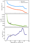 |
Fig. 6. Evolution of the bolometric and pseudo-bolometric luminosity (top panel), photospheric temperature (central), and photospheric radius (bottom) of SN 2024bch derived with SuperBol. We highlight the values of temperature and radius reached at ∼20 days after the explosion. |
All the other parameters shown in Table 2 are obtained with CASTOR v2.0, based on the luminosity curve derived with SuperBol. Parameters are estimated applying analytical models directly on the luminosity curve, assuming the most general physical framework, such as spherical and isotropic explosion, perfect adiabacity at peak luminosity and a modified black-body law of emission. The energy partition is based on the SN 1987A model, with a canonical 99.9% of the total energy transported by neutrinos and 0.1% by photons. For a detailed overview on how every parameter is derived and the inter-degeneracies between parameters, see Simongini et al. (2024).
Parametric map of SN 2024bch: general parameters of the event, properties of the ejecta, properties of the photosphere, and main parameters of the progenitor star.
Among the estimated parameters, this analysis allows us to constrain the mass and the radius of the progenitor star. The progenitor’s mass is derived from the mass of the ejecta, assuming perfect conservation of mass at explosion and assuming two possible values for the remnant, effectively creating an interval of possible values. We obtained Mpr = 11–20 M⊙. This interval overlaps with previous estimations from Tartaglia et al. (2024), who reported a possible progenitor mass in the range 15–18 M⊙, and Andrews et al. (2025) who assumed a value of 15 M⊙ to model the spectral evolution of the SN. Taken together with previous studies, our result supports the conclusion that the progenitor mass was likely around 15 M⊙. On the other hand, the progenitor’s radius is constrained using the scaling relation from Shussman et al. (2016):
 (5)
(5)
where ET is time-weighted integrated bolometric luminosity (e.g., Katz et al. 2013; Nakar et al. 2016; Zimmerman et al. 2024) and Mej is the mass of the ejecta. We obtain Rpr = 531 ± 125 R⊙, similar to the assumed value of Rpr = 501 R⊙ from Andrews et al. (2025).
4.3. Pre-explosion image
We analyzed one image of the host-galaxy of SN 2024bch prior to the explosion, taken with the Hubble Space Telescope2 on May 14, 2001 (Fig. 7). The region around the coordinates of the explosion appears more luminous than the background, significantly above the magnitude limit of the map. Table 3 collects the properties of the candidate progenitor stars identified by different photometric catalogs. The small differences in the coordinates might be attributed to the different techniques used and astrometric errors. Therefore, we assumed that all the catalogs identify the same candidate. However, even if they correspond to different sources, our estimations remain valid. The apparent magnitudes are converted into luminosity using the host-galaxy distance and rescaled with respect to the solar luminosity with a base-10 logarithm. Hence, the different catalogs identify a candidate star with a luminosity at most between Lpr = 103.81 and 104.82 L⊙. Using the Stefan-Boltzmann law, this luminosity interval corresponds to an effective temperature in the range between Tpr = 2000 and 4000 K.
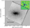 |
Fig. 7. Location of SN 2024bch in its host galaxy, NGC 3206. This pre-explosion image was taken by the Hubble Space Telescope on May 14, 2001, almost 20 years before the explosion. We zoom in on the region around the coordinates of SN 2024bch (white star), where different stars are identified as candidate progenitors (red crosses), and use a different color-map to highlight the S/N. |
Pre-explosion parameters of the candidate progenitor of SN 2024bch.
5. On the supernova type and the progenitor star
After the luminosity peak, SN 2024bch light curves decay linearly within the following ∼ tens of days, in good agreement with the definition of type II-L SNe. We found this behavior to be similar to the ones showed by SN 2009kr, SN 2013fc, and SN 2008fq. Apart from SN 2009kr, which was classified as a II-L (Elias-Rosa et al. 2010), SN 2013fc and SN 2008fq belong to the subgroup of type IIn-L SNe (Taddia et al. 2013; Kangas et al. 2016).
We took the adopted values of reddening and distance into account to determine the absolute magnitudes (see Fig. 3). The absorption relative to every filter is obtained using the prescriptions from McCall (2004). The V band rises to its peak value, −17.64 ± 0.13, within the first 10 days after the explosion. In the same period, the B band reaches a value of −17.84 ± 0.14 and the R band a value of −17.44 ± 0.13. The quick rise is similar to that of other IIn objects (e.g., SN 1998S, SN 2007pk, and SN 2008fq), as is the V-band peak brightness (−18.5 < Vmax < −19.3; Taddia et al. 2013) despite being under-luminous. Nevertheless, the B-band maximum aligns with the average value of type II-L (−17.98 ± 0.34; Richardson et al. 2014). Note that our values are slightly lower than the ones reported in Andrews et al. (2025) due to the different adopted distance. Moreover, as shown in Fig. 3, the plateau lasts for about ∼70 days, consistent with the low end of the II-L distribution reported in Valenti et al. (2015). The early-time spectra exhibit weak signatures of CSM interaction in the form of narrow and weak Hα profiles, which seem to disappear soon after the peak of luminosity in favor of broad and strong lines at later times. Furthermore, SN 2024bch was originally classified as IIn due to the spectral similarity to SN 1998S using the classification software GELATO (Harutyunyan et al. 2008). Hence, the overall spectro-photometric behavior of SN 2024bch resembles that of CSI interacting type IIn-L SNe.
We found for the progenitor star Mpr = (11 − 20) M⊙, Rpr = 531 ± 125 R⊙, Lpr ≤ 104.82 L⊙, and Tpr ≤ 4000 K from optical modeling and pre-explosion images and Ṁ ≤ 10−3 M⊙ yr−1 assuming uw = 10 km s−1 from gamma-ray studies. According to Taddia et al. (2015), who studied the metallicity levels in the explosion sites of different CSI SNe, the progenitor stars of type IIn-L SNe are more likely RSGs, as for II-P and II-L SNe. These are among the most common progenitors for type II SNe. Typical RSGs have masses between 8 and 20 M⊙, radii up to 1500 R⊙ and luminosities between 104 and 105 L⊙ for the brightest objects (Smartt 2015). The different rate of occurrence between II-L and II-P events suggests that the progenitors of II-L are somehow more massive and thus more luminous than those of II-P progenitors (Branch & Wheeler 2017). Moreover, RSGs have relatively low wind velocity (uw ∼ 10 km s−1) and mass loss rates in the range 10−6 – 10−4 M⊙ yr−1. Mackey et al. (2014) proposed the possibility of RSGs being progenitors for CSI SNe in the presence of nearby hot stars. The companion star can photo-ionize up to 35% of the gas lost by the RSG during its lifetime, forming a dense and confined shell around it. When the star explodes, the ejecta will interact with the dense shell, producing the characteristic features of type IIn SNe. Based on the result achieved by our analysis, we might infer that the progenitor star parameters agree with the RSG scenario, as also supported by the spectro-photometric behavior. This scenario was also explored by Andrews et al. (2025) who, assuming a progenitor star of M = 15 M⊙, found a wind velocity of 35 – 40 km s−1 and a mass-loss-rate of Ṁ = 10−3 − 10−2, consistent with our estimate.
However, the LBV scenario cannot be ruled out, as LBVs are most likely to be progenitors for IIn explosion (e.g., Gal-Yam & Leonard 2009; Mauerhan et al. 2013). LBVs are among the most luminous stars known (L ∼ 105–108 L⊙) with high masses in the range M = 20–80 M⊙. They undergo episodic outbursts with significant mass losses of about 10−3–10−2 M⊙ yr−1 (Taddia et al. 2013) for relatively high wind velocities (uw ∼ 102 km s−1). Hence, the progenitor properties derived in this study might also indicate a LBV progenitor at the lower edge of the typical mass and luminosity spectrum, although this appears to be a less likely scenario.
6. On the attenuation problem
At the time of writing, a comprehensive model for accurately defining the impact and timescale on which gamma-gamma interactions might attenuate the VHE flux to the point of being undetectable is missing. Current models adopt different approaches, often considering distinct parameter contributions, leading to various possible scenarios that strongly depend on the system’s geometry and whether its evolution is treated as time-dependent or time-independent (e.g., Cristofari et al. 2020). In a recent work, Cristofari et al. (2022) modeled the gamma-ray emission of a typical II-P SN with results depending on the total explosion energy, the mass-loss rate of the pre-SN wind, the wind terminal velocity, the mass of the ejecta and the radius of the progenitor star. They show how the gamma-gamma attenuation significantly affects the flux above 100 GeV at early times (between 0 and 12 days), by potentially suppressing the expected VHE flux by about 20 orders of magnitude. However, the impact of this attenuation decreases with time, and at 12 days it can lower the effective flux by 1 to 5 orders of magnitude depending on the combination of the various parameters. Similarly, Brose et al. (2022) simulated the emission from II-P and IIn SNe associated with RSG and LBV progenitor stars, respectively, in the H.E.S.S. and Fermi-LAT energy ranges. In both cases the gamma-gamma absorption can effectively suppress the flux at early times, with the effect being more pronounced at energies above 1 TeV. The gamma-ray luminosity can potentially be attenuated by 3 orders of magnitude at most at 15 days depending on the relative mass-loss rate. After the peak of luminosity, the effect can still be relevant up to ∼ 220 days.
A significant factor in modeling gamma-gamma absorption is the evolution of the photosphere. As shown in Fig. 6, the SN photosphere undergoes rapid cooling between the time of explosion and the bulk of the LST-1 observations, with its temperature decreasing by a factor of 2. Meanwhile, the radius expands almost linearly in the first days, with a sudden change of slope around day 15, possibly caused by a decoupling between the shock and the photospheric radius. This feature coincides with the onset of a decline in the pseudo-bolometric luminosity. These changes suggest that the optical target photon field becomes less dense during the bulk of LST-1 observations, supporting the approximation that absorbed and unabsorbed fluxes are approximately coincident in this phase. More broadly, the relatively rapid decline in optical luminosity observed in type II-L SNe may imply systematically weaker gamma-gamma absorption compared to the more extended plateau phase of type II-P SNe. However, a more quantitative description would require a dedicated model based on the observed evolution, which is beyond the scope of this work.
Based on these considerations, it is possible that the gamma-flux observations of SN 2024bch cannot be directly converted to mass-loss ULs due to the role of the gamma-gamma attenuation. The LST-1 observations were performed starting at t0 + 16, with the bulk of observations clustered around 20 days after the explosion, when the impact of gamma-gamma absorption may still have been relevant, attenuating the flux for a factor of three orders of magnitude at most. Considering these three levels of attenuation, our flux UL would translate to a weaker mass-loss-rate to wind-velocity ratio UL. In particular, assuming Fabs = 10−xFunabs, where x = 1, 2, 3, we obtain ![Mathematical equation: $ \dot M/u_\text{w} \le [0.38, 1.2, 3.8] \times 10^{-3} \frac{\text{ M}_\odot}{\text{ yr}}\frac{\text{ s}}{\text{ km}} $](/articles/aa/full_html/2025/10/aa54721-25/aa54721-25-eq9.gif) , respectively.
, respectively.
7. Conclusions
We have presented a multiwavelength analysis of SN 2024bch. We conducted a follow-up campaign at VHE gamma rays with the LST-1 and in the optical with the LT. No detection was achieved in the VHE band, and we computed the corresponding ULs for the six nights of observation with the LST-1. To interpret such ULs in a physical context, we considered the model from Dwarkadas (2013), estimating ULs for the ratio of the mass-loss rate to the wind velocity. Moreover, we performed an optical analysis, employing one spectrum observed with the LT complemented with ancillary data from online public repositories for both photometry and spectroscopy. We used the open-source software SuperBol (Nicholl 2018) to study the photospheric evolution of SN 2024bch and the software CASTOR (Simongini et al. 2024) to estimate the parameters of the event and to compare SN 2024bch light curves with those of other known events. Furthermore, we analyzed a pre-explosion image of SN 2024bch from the Hubble Space Legacy Archive. Our major findings are as follows:
-
The integrated photon flux UL of SN 2024bch above 100 GeV is Fγ(> 100 GeV)≤3.61 × 10⁻¹² cm−2 s−1, as obtained from 12 h of LST-1 observations; this is coincident with a luminosity UL of Lγ ≤ 1.33 × 1041erg s−1. These ULs align with those of other types of SNe found by Abdalla et al. (2019), Ahnen et al. (2017), and Acharyya et al. (2023). However, none of the cited works included IIn-L SNe. Therefore, this is the first ever determined gamma-flux UL for a SN of this class, and the first ever observation of a CCSN by an IACT with such a low energy threshold.
-
SN 2024bch was likely a type IIn-L SN according to several pieces of evidence. The light curves show a fast linear decay typical of type II-L SNe; the spectra evolve from IIn-like to IIL-like, with narrow and weak H−α profiles at early times that disappear after the peak of luminosity in favor of broad and strong lines at later times. According to Tartaglia et al. (2024), the narrow features disappeared between day 16 and day 42 after the explosion. We find the photometric behavior to be similar to that of SN 2009kr, SN 2013fc, and SN 2008fq, while an independent classification made by Balcon (2024), performed around 3.5 days after the explosion, suggests a spectral similarity to SN 1998S.
-
The SN 2024bch progenitor was likely a RSG according to our estimated parameters. From independent analyses we found Mpr = (11–20) M⊙, Rpr = 531 ± 125 R⊙,
 , Tpr ≤ 4000 K, and
  , all of which are in good agreement with the typical values of these stars. The RSG progenitor channel is also supported by the classification, as type IIn-L SN explosion sites are found to be more similar to those of type II-L progenitors than those of type IIn (Taddia et al. 2015).
Based on our interpretation, SN 2024bch belongs to the IIn-L SN class. Moreover, our results, in line with the existing literature, strongly suggest a RSG progenitor, although we cannot exclude the LBV progenitor channel. The uncertainty regarding the preferred progenitor channel for SN 2024bch highlights the crucial role of the mass-loss rate estimate. Future observations of SNe at VHEs will eventually reveal the elusive signal, enabling a more accurate modeling of the incoming flux and more constraining results.
Acknowledgments
We gratefully acknowledge financial support from the following agencies and organisations: Conselho Nacional de Desenvolvimento Científico e Tecnológico (CNPq), Fundação de Amparo à Pesquisa do Estado do Rio de Janeiro (FAPERJ), Fundação de Amparo à Pesquisa do Estado de São Paulo (FAPESP), Fundação de Apoio à Ciência, Tecnologia e Inovação do Paraná – Fundação Araucária, Ministry of Science, Technology, Innovations and Communications (MCTIC), Brasil; Ministry of Education and Science, National RI Roadmap Project DO1-153/28.08.2018, Bulgaria; Croatian Science Foundation (HrZZ) Project IP-2022-10-4595, Rudjer Boskovic Institute, University of Osijek, University of Rijeka, University of Split, Faculty of Electrical Engineering, Mechanical Engineering and Naval Architecture, University of Zagreb, Faculty of Electrical Engineering and Computing, Croatia; Ministry of Education, Youth and Sports, MEYS LM2023047, EU/MEYS CZ.02.1.01/0.0/0.0/16_013/0001403, CZ.02.1.01/0.0/0.0/18_046/0016007, CZ.02.1.01/0.0/0.0/16_019/0000754, CZ.02.01.01/00/22_008/0004632 and CZ.02.01.01/00/23_015/0008197 Czech Republic; CNRS-IN2P3, the French Programme d’investissements d’avenir and the Enigmass Labex, This work has been done thanks to the facilities offered by the Univ. Savoie Mont Blanc – CNRS/IN2P3 MUST computing center, France; Max Planck Society, German Bundesministerium für Bildung und Forschung (Verbundforschung/ErUM), Deutsche Forschungsgemeinschaft (SFBs 876 and 1491), Germany; Istituto Nazionale di Astrofisica (INAF), Istituto Nazionale di Fisica Nucleare (INFN), Italian Ministry for University and Research (MUR), and the financial support from the European Union – Next Generation EU under the project IR0000012 - CTA+ (CUP C53C22000430006), announcement N.3264 on 28/12/2021: “Rafforzamento e creazione di IR nell’ambito del Piano Nazionale di Ripresa e Resilienza (PNRR)”; ICRR, University of Tokyo, JSPS, MEXT, Japan; JST SPRING – JPMJSP2108; Narodowe Centrum Nauki, grant number 2019/34/E/ST9/00224, Poland; The Spanish groups acknowledge the Spanish Ministry of Science and Innovation and the Spanish Research State Agency (AEI) through the government budget lines PGE2022/28.06.000X.711.04, 28.06.000X.411.01 and 28.06.000X.711.04 of PGE 2023, 2024 and 2025, and grants PID2019-104114RB-C31, PID2019-107847RB-C44, PID2019-104114RB-C32, PID2019-105510GB-C31, PID2019-104114RB-C33, PID2019-107847RB-C43, PID2019-107847RB-C42, PID2019-107988GB-C22, PID2021-124581OB-I00, PID2021-125331NB-I00, PID2022-136828NB-C41, PID2022-137810NB-C22, PID2022-138172NB-C41, PID2022-138172NB-C42, PID2022-138172NB-C43, PID2022-139117NB-C41, PID2022-139117NB-C42, PID2022-139117NB-C43, PID2022-139117NB-C44, PID2022-136828NB-C42, PDC2023-145839-I00 funded by the Spanish MCIN/AEI/10.13039/501100011033 and “and by ERDF/EU and NextGenerationEU PRTR; the “Centro de Excelencia Severo Ochoa” program through grants no. CEX2019-000920-S, CEX2020-001007-S, CEX2021-001131-S; the “Unidad de Excelencia María de Maeztu” program through grants no. CEX2019-000918-M, CEX2020-001058-M; the “Ramón y Cajal” program through grants RYC2021-032991-I funded by MICIN/AEI/10.13039/501100011033 and the European Union “NextGenerationE”/PRTR and RYC2020-028639-I; the “Juan de la Cierva-Incorporación” program through grant no. IJC2019-040315-I and “Juan de la Cierva-formación” through grant JDC2022-049705-I. They also acknowledge the “Atracción de Talento” program of Comunidad de Madrid through grant no. 2019-T2/TIC-12900; the project “Tecnologías avanzadas para la exploración del universo y sus componentes” (PR47/21 TAU), funded by Comunidad de Madrid, by the Recovery, Transformation and Resilience Plan from the Spanish State, and by NextGenerationEU from the European Union through the Recovery and Resilience Facility; “MAD4SPACE: Desarrollo de tecnologías habilitadoras para estudios del espacio en la Comunidad de Madrid” (TEC-2024/TEC-182) project funded by Comunidad de Madrid; the La Caixa Banking Foundation, grant no. LCF/BQ/PI21/11830030; Junta de Andalucía under Plan Complementario de I+D+I (Ref. AST22_0001) and Plan Andaluz de Investigación, Desarrollo e Innovación as research group FQM-322; Project ref. AST22_00001_9 with funding from NextGenerationEU funds; the “Ministerio de Ciencia, Innovación y Universidades” and its “Plan de Recuperación, Transformación y Resiliencia”; “Consejería de Universidad, Investigación e Innovación” of the regional government of Andalucía and “Consejo Superior de Investigaciones Científicas”, Grant CNS2023-144504 funded by MICIU/AEI/10.13039/501100011033 and by the European Union NextGenerationEU/PRTR, the European Union’s Recovery and Resilience Facility-Next Generation, in the framework of the General Invitation of the Spanish Government’s public business entity Red.es to participate in talent attraction and retention programmes within Investment 4 of Component 19 of the Recovery, Transformation and Resilience Plan; Junta de Andalucía under Plan Complementario de I+D+I (Ref. AST22_00001), Plan Andaluz de Investigación, Desarrollo e Innovación (Ref. FQM-322). “Programa Operativo de Crecimiento Inteligente” FEDER 2014-2020 (Ref. ESFRI-2017-IAC-12), Ministerio de Ciencia e Innovación, 15% co-financed by Consejería de Economía, Industria, Comercio y Conocimiento del Gobierno de Canarias; the “CERCA” program and the grants 2021SGR00426 and 2021SGR00679, all funded by the Generalitat de Catalunya; and the European Union’s NextGenerationEU (PRTR-C17.I1). This research used the computing and storage resources provided by the Port d’Informació Científica (PIC) data center. State Secretariat for Education, Research and Innovation (SERI) and Swiss National Science Foundation (SNSF), Switzerland; The research leading to these results has received funding from the European Union’s Seventh Framework Programme (FP7/2007-2013) under grant agreements No 262053 and No 317446; This project is receiving funding from the European Union’s Horizon 2020 research and innovation programs under agreement No 676134; ESCAPE – The European Science Cluster of Astronomy & Particle Physics ESFRI Research Infrastructures has received funding from the European Union’s Horizon 2020 research and innovation programme under Grant Agreement no. 824064. We acknowledge with thanks the variable star observations from the AAVSO International Database contributed by observers worldwide and used in this research. Based on observations made with the NASA/ESA Hubble Space Telescope, and obtained from the Hubble Legacy Archive, which is a collaboration between the Space Telescope Science Institute (STScI/NASA), the Space Telescope European Coordinating Facility (ST-ECF/ESA) and the Canadian Astronomy Data Centre (CADC/NRC/CSA). This article is also based on observations made in the Liverpool telescope located at the Observatorio del Roque de los Muchachos under the CL24A06 (PI: A. López-Oramas) program. This research is part of the Project RYC2021-032991-I, funded by MICIN/AEI/10.13039/501100011033, and the European Union “NextGenerationEU”/PRTR. Author contribution: A. Simongini: project coordination, LST-1 data analysis, optical data analysis, model fitting, physical interpretation, paper drafting and edition; A. López-Oramas: PI of the LST-1 proposal, PI of the LT proposal, discussion of the model and of the obtained results, paper edition; A. Carosi: discussion of the model and of the obtained results, paper edition; A. Aguasca-Cabot: LST-1 data analysis, paper edition. The rest of the authors have contributed in one or several of the following ways: design, construction, maintenance and operation of the instrument(s) used to acquire the data; preparation and/or evaluation of the observation proposals; data acquisition, processing, calibration and/or reduction; production of analysis tools and/or related Monte Carlo simulations; discussion and approval of the contents of the draft.
References
- Abdalla, H., Aharonian, F., Benkhali, F. A., et al. 2019, A&A, 626, A57 [NASA ADS] [CrossRef] [EDP Sciences] [Google Scholar]
- Abe, H., Abe, K., Abe, S., et al. 2023a, A&A, 680, A66 [CrossRef] [EDP Sciences] [Google Scholar]
- Abe, H., Abe, K., Abe, S., et al. 2023b, ApJ, 956, 80 [CrossRef] [Google Scholar]
- Acero, F., Bernete, J., Biederbeck, N., et al. 2024, https://doi.org/10.5281/zenodo.10726484 [Google Scholar]
- Acharyya, A., Adams, C. B., Bangale, P., et al. 2023, ApJ, 945, 30 [Google Scholar]
- Ahnen, M. L., Ansoldi, S., Antonelli, L. A., et al. 2017, A&A, 602, A98 [NASA ADS] [CrossRef] [EDP Sciences] [Google Scholar]
- Anderson, J. P., González-Gaitán, S., Hamuy, M., et al. 2014, ApJ, 786, 67 [Google Scholar]
- Andrews, J. E., Shrestha, M., Bostroem, K. A., et al. 2025, ApJ, 980, 37 [Google Scholar]
- Balcon, C. 2024, Transient Name Server Classification Report, 2024-284, 1 [Google Scholar]
- Barbon, R., Ciatti, F., & Rosino, L. 1979, A&A, 72, 287 [Google Scholar]
- Bell, A., Schure, K., Reville, B., & Giacinti, G. 2013, MNRAS, 431, 415 [NASA ADS] [CrossRef] [Google Scholar]
- Bionta, R. M., Blewitt, G., Bratton, C. B., et al. 1987, Phys. Rev. Lett., 58, 1494 [Google Scholar]
- Bošnjak, Ž., Brown, A. M., Carosi, A., et al. 2021, ArXiv e-prints [arXiv:2106.03621] [Google Scholar]
- Branch, D., & Wheeler, J. C. 2017, Supernova explosions (Springer), 4 [Google Scholar]
- Brose, R., Sushch, I., & Mackey, J. 2022, MNRAS, 516, 492 [NASA ADS] [CrossRef] [Google Scholar]
- Bykov, A., Ellison, D., Marcowith, A., & Osipov, S. 2018, Space Sci. Rev., 214, 1 [NASA ADS] [CrossRef] [Google Scholar]
- Castignani, G., Vulcani, B., Finn, R. A., et al. 2022, ApJS, 259, 43 [NASA ADS] [CrossRef] [Google Scholar]
- Chen, P., Gal-Yam, A., Sollerman, J., et al. 2024, Nature, 625, 253 [NASA ADS] [CrossRef] [Google Scholar]
- Cherenkov Telescope Array Consortium (Acharya, B. S., et al.) 2019, Science with the Cherenkov Telescope Array [Google Scholar]
- Chevalier, R. A. 1982, ApJ, 259, 302 [Google Scholar]
- Chevalier, R. A., & Fransson, C. 1994, ApJ, 420, 268 [NASA ADS] [CrossRef] [Google Scholar]
- Chevalier, R. A., & Fransson, C. 2017, Handbook of supernovae (Springer), 1 [Google Scholar]
- Chugai, N. 2001, MNRAS, 326, 1448 [NASA ADS] [CrossRef] [Google Scholar]
- Cold, C., & Hjorth, J. 2023, A&A, 670, A48 [NASA ADS] [CrossRef] [EDP Sciences] [Google Scholar]
- Cristofari, P., Renaud, M., Marcowith, A., Dwarkadas, V. V., & Tatischeff, V. 2020, MNRAS, 494, 2760 [NASA ADS] [CrossRef] [Google Scholar]
- Cristofari, P., Marcowith, A., Renaud, M., et al. 2022, MNRAS, 511, 3321 [Google Scholar]
- Donath, A., Terrier, R., Remy, Q., et al. 2023, A&A, 678, A157 [NASA ADS] [CrossRef] [EDP Sciences] [Google Scholar]
- Drury, L. O., Aharonian, F. A., & Voelk, H. J. 1994, A&A, 287, 959 [NASA ADS] [Google Scholar]
- Dwarkadas, V. V. 2013, MNRAS, 434, 3368 [NASA ADS] [CrossRef] [Google Scholar]
- Elias-Rosa, N., Van Dyk, S. D., Li, W., et al. 2010, ApJ, 714, L254 [Google Scholar]
- Faran, T., Poznanski, D., Filippenko, A., et al. 2014, MNRAS, 445, 554 [NASA ADS] [CrossRef] [Google Scholar]
- Fassia, A., Meikle, W., Chugai, N., et al. 2001, MNRAS, 325, 907 [NASA ADS] [CrossRef] [Google Scholar]
- Filippenko, A. V. 1997, ARA&A, 35, 309 [NASA ADS] [CrossRef] [Google Scholar]
- Fomin, V., Stepanian, A., Lamb, R., et al. 1994, Astropart. Phys., 2, 137 [NASA ADS] [CrossRef] [Google Scholar]
- Fransson, C., Chevalier, R. A., Filippenko, A. V., et al. 2002, AJ, 572, 350 [Google Scholar]
- Gall, E. E. E., Polshaw, J., Kotak, R., et al. 2015, A&A, 582, A3 [NASA ADS] [CrossRef] [EDP Sciences] [Google Scholar]
- Gal-Yam, A., & Leonard, D. C. 2009, Nature, 458, 865 [NASA ADS] [CrossRef] [Google Scholar]
- Habergham, S., Anderson, J., James, P., & Lyman, J. 2014, MNRAS, 441, 2230 [CrossRef] [Google Scholar]
- Harutyunyan, A., Pfahler, P., Pastorello, A., et al. 2008, A&A, 488, 383 [NASA ADS] [CrossRef] [EDP Sciences] [Google Scholar]
- Hirata, K., Kajita, T., Koshiba, M., et al. 1987, Phys. Rev. Lett., 58, 1490 [NASA ADS] [CrossRef] [Google Scholar]
- Kangas, T., Mattila, S., Kankare, E., et al. 2016, MNRAS, 456, 323 [NASA ADS] [CrossRef] [Google Scholar]
- Katz, B., Kushnir, D., & Dong, S. 2013, ArXiv e-prints [arXiv:1301.6766] [Google Scholar]
- Kloppenborg, B. K. 2024, Observations from the AAVSO International Database https://www.aavso.org [Google Scholar]
- Kotak, R., & Vink, J. S. 2006, A&A, 460, L5 [NASA ADS] [CrossRef] [EDP Sciences] [Google Scholar]
- Li, W., Leaman, J., Chornock, R., et al. 2011, MNRAS, 412, 1441 [NASA ADS] [CrossRef] [Google Scholar]
- Longair, M. S. 2011, High energy astrophysics (Cambridge University Press) [Google Scholar]
- López-Coto, R., Moralejo, A., Artero, M., et al. 2021, Proc. 37th Int. Cosmic Ray Conf., 395, 806 [Google Scholar]
- Lopez-Coto, R., Vuillaume, T., Moralejo, A., et al. 2024, https://doi.org/10.5281/zenodo.10604579 [Google Scholar]
- Mackey, J., Mohamed, S., Gvaramadze, V. V., et al. 2014, Nature, 512, 282 [Google Scholar]
- Marcowith, A., Dwarkadas, V. V., Renaud, M., Tatischeff, V., & Giacinti, G. 2018, MNRAS, 479, 4470 [CrossRef] [Google Scholar]
- Mauerhan, J. C., Smith, N., Filippenko, A. V., et al. 2013, MNRAS, 430, 1801 [NASA ADS] [CrossRef] [Google Scholar]
- McCall, M. L. 2004, AJ, 128, 2144 [Google Scholar]
- Murase, K. 2024, Phys. Rev. D, 109, 103020 [CrossRef] [Google Scholar]
- Murase, K., Thompson, T. A., Lacki, B. C., & Beacom, J. F. 2011, Phys. Rev. D Part. Fields Gravit. Cosmol., 84, 043003 [Google Scholar]
- Nakar, E., Poznanski, D., & Katz, B. 2016, ApJ, 823, 127 [CrossRef] [Google Scholar]
- Nicholl, M. 2018, RNAAS, 2, 230 [Google Scholar]
- Patat, F., Barbon, R., Cappellaro, E., & Turatto, M. 1994, A&A, 282, 731 [NASA ADS] [Google Scholar]
- Piascik, A. S., Steele, I. A., Bates, S. D., et al. 2014, SPIE Conf. Ser., 9147, 91478H [NASA ADS] [Google Scholar]
- Pozzo, M., Meikle, W., Fassia, A., et al. 2004, MNRAS, 352, 457 [CrossRef] [Google Scholar]
- Richardson, D., Jenkins, R. L., III, Wright, J., & Maddox, L. 2014, AJ, 147, 118 [NASA ADS] [CrossRef] [Google Scholar]
- Sanders, N. E., Soderberg, A. M., Gezari, S., et al. 2015, ApJ, 799, 208 [NASA ADS] [CrossRef] [Google Scholar]
- Schlegel, E. M. 1990, MNRAS, 244, 269 [NASA ADS] [Google Scholar]
- Shussman, T., Nakar, E., Waldman, R., & Katz, B. 2016, ArXiv e-prints [arXiv:1602.02774] [Google Scholar]
- Simongini, A., Ragosta, F., Piranomonte, S., & Di Palma, I. 2024, MNRAS, 533, 3053 [Google Scholar]
- Simongini, A., Ragosta, F., Piranomonte, S., & Di Palma, I. 2025, CASTOR: v2.0 - 2025–03-05 [Google Scholar]
- Smartt, S. 2015, PASA, 32, e016 [NASA ADS] [CrossRef] [Google Scholar]
- Smith, N. 2017, Handbook of supernovae (Springer), 403 [Google Scholar]
- Smith, N., Hinkle, K. H., & Ryde, N. 2009, AJ, 137, 3558 [NASA ADS] [CrossRef] [Google Scholar]
- Steele, I. A., Smith, R. J., Rees, P. C., et al. 2004, SPIE, 5489, 679 [NASA ADS] [Google Scholar]
- Taddia, F., Stritzinger, M., Sollerman, J., et al. 2013, A&A, 555, A10 [NASA ADS] [CrossRef] [EDP Sciences] [Google Scholar]
- Taddia, F., Sollerman, J., Fremling, C., et al. 2015, A&A, 580, A131 [NASA ADS] [CrossRef] [EDP Sciences] [Google Scholar]
- Tartaglia, L., Valerin, G., Pastorello, A., et al. 2024, A&A, submitted [arXiv:2409.15431] [Google Scholar]
- Tatischeff, V. 2009, A&A, 499, 191 [NASA ADS] [CrossRef] [EDP Sciences] [Google Scholar]
- Trundle, C., Kotak, R., Vink, J. S., & Meikle, W. P. S. 2008, A&A, 483, L47 [NASA ADS] [CrossRef] [EDP Sciences] [Google Scholar]
- Tully, R. B., Courtois, H. M., & Sorce, J. G. 2016, AJ, 152, 50 [Google Scholar]
- Valenti, S., Sand, D., Stritzinger, M., et al. 2015, MNRAS, 448, 2608 [NASA ADS] [CrossRef] [Google Scholar]
- Wiggins, P. 2024, Transient Name Server Discovery Report, 2024–281, 1 [Google Scholar]
- Xi, S.-Q., Liu, R.-Y., Wang, X.-Y., et al. 2020, ApJ, 896, L33 [NASA ADS] [CrossRef] [Google Scholar]
- Yaron, O., & Gal-Yam, A. 2012, PASP, 124, 668 [Google Scholar]
- Yuan, Q., Liao, N.-H., Xin, Y.-L., et al. 2018, ApJ, 854, L18 [NASA ADS] [CrossRef] [Google Scholar]
- Zimmerman, E. A., Irani, I., Chen, P., et al. 2024, Nature, 627, 759 [Google Scholar]
All Tables
Parametric map of SN 2024bch: general parameters of the event, properties of the ejecta, properties of the photosphere, and main parameters of the progenitor star.
All Figures
|
Fig. 1. LST-1 differential ULs obtained from SN 2024bch observations between 75 GeV and 10 TeV, estimated with three energy bins per decade and assuming a fixed spectral index of –2.5 considering the full time-range. ULs are computed with a 2σ confidence level. |
| In the text | |
|
Fig. 2. ULs for the gamma-ray light curves of SN 2024bch, computed between 100 GeV and 10 TeV. We compare the night-wise ULs (blue) with the integrated UL, obtained by stacking all results together (red). The gray-shaded area covers the nights with strong moonlight. ULs are computed with a 2σ confidence level. |
| In the text | |
|
Fig. 3. Public photometry of SN 2024bch (filled points). We used observations in the four filters B, V, R, and I. An offset is added to the data points for a better visualization. Solid lines are the result of GP interpolation obtained with CASTOR (see the main text). The uncertainties of the interpolated lines are shown as shaded contours. The vertical solid black lines show the LST-1 observation windows. |
| In the text | |
|
Fig. 4. Comparison of the BVR light curves of SN 2024bch (blue dots) with those of SN 2009kr and SN 2013fc (dashed red and green curves, respectively). The data for SN 2009kr and SN 2013fc are scaled to match SN 2024bch and interpolated over the same time interval using GP interpolation (see the main text for details). Additionally, we show a reference curve representing a decay of 1 magnitude between tmax and t50. |
| In the text | |
|
Fig. 5. Spectra of SN 2024bch compared with two spectra of SN 2013fc (at 17 and 51 days post-explosion) and two spectra of SN 2008fq (at 6 and 57 days post-explosion). We removed the continuum from every spectrum and normalized to order zero. We added an offset for better visualization. The main spectral features of SN 2024bch are highlighted as purple-shaded vertical bands. Telluric lines are identified as “T1” and “T2” (gray bands). The spectrum taken with LT is the second from the bottom of the SN 2024bch spectra, at 47 days post-explosion. The other spectral data for the three SNe are taken from WISeREP (Yaron & Gal-Yam 2012). |
| In the text | |
|
Fig. 6. Evolution of the bolometric and pseudo-bolometric luminosity (top panel), photospheric temperature (central), and photospheric radius (bottom) of SN 2024bch derived with SuperBol. We highlight the values of temperature and radius reached at ∼20 days after the explosion. |
| In the text | |
|
Fig. 7. Location of SN 2024bch in its host galaxy, NGC 3206. This pre-explosion image was taken by the Hubble Space Telescope on May 14, 2001, almost 20 years before the explosion. We zoom in on the region around the coordinates of SN 2024bch (white star), where different stars are identified as candidate progenitors (red crosses), and use a different color-map to highlight the S/N. |
| In the text | |
Current usage metrics show cumulative count of Article Views (full-text article views including HTML views, PDF and ePub downloads, according to the available data) and Abstracts Views on Vision4Press platform.
Data correspond to usage on the plateform after 2015. The current usage metrics is available 48-96 hours after online publication and is updated daily on week days.
Initial download of the metrics may take a while.