| Issue |
A&A
Volume 702, October 2025
|
|
|---|---|---|
| Article Number | A134 | |
| Number of page(s) | 16 | |
| Section | Extragalactic astronomy | |
| DOI | https://doi.org/10.1051/0004-6361/202555078 | |
| Published online | 15 October 2025 | |
Analyzing Type Ia supernovae near-infrared light curves with principal component analysis
1
Institute of Space Sciences (ICE, CSIC), Campus UAB, Carrer de Can Magrans, s/n, E-08193 Barcelona, Spain
2
Institut d’Estudis Espacials de Catalunya (IEEC), E-08034 Barcelona, Spain
3
School of Physics, Trinity College Dublin, The University of Dublin, Dublin 2, Ireland
4
Instituto de Ciencias Exactas y Naturales (ICEN), Universidad Arturo Prat, Chile
5
Department of Physics and Astronomy, Aarhus University, Ny Munkegade 120, DK-8000 Aarhus C, Denmark
6
Institute for Astronomy, University of Hawai’i, 2680 Woodlawn Drive, Honolulu HI 96822, USA
7
Planetary Science Institute, 1700 E Fort Lowell Rd., Ste 106, Tucson AZ 85719, USA
8
Hamburger Sternwarte, Gojensbergweg 112, 21029 Hamburg, Germany
9
Observatories of the Carnegie Institution for Science, 813 Santa Barbara Street, Pasadena CA 91101, USA
10
Department of Physics, Florida State University, Tallahassee 32306, USA
11
Las Campanas Observatory, Carnegie Observatories, Casilla 601, La Serena, Chile
12
George P. and Cynthia Woods Mitchell Institute for Fundamental Physics and Astronomy, Department of Physics and Astronomy, Texas A&M University, College Station, TX 77843, USA
13
Center for Astronomy, Space Science and Astrophysics, Independent University, Bangladesh Dhaka 1245, Bangladesh
14
American Public University System, Charles Town, WV 25414, USA
⋆ Corresponding author: This email address is being protected from spambots. You need JavaScript enabled to view it.
Received:
8
April
2025
Accepted:
8
August
2025
Abstract
Thermonuclear explosions of C/O white dwarf stars in binary systems known as Type Ia supernovae (SNe Ia) remain poorly understood. The complexity of their progenitor systems, explosion physics, and intrinsic diversity poses challenges in understanding these phenomena as astrophysical objects, as well as their standardization and use as cosmological probes. Near-infrared (NIR) observations offer a promising avenue for studying the physics of SNe Ia and for reducing systematic uncertainties in distance estimations, as they exhibit lower dust extinction and smaller dispersion in peak luminosity than optical bands. In this work, we applied a principal component analysis (PCA) to a sample of SNe Ia with well-sampled NIR (YJH-band) light curves to identify the dominant components of their variability and constrain physical underlying properties. The theoretical models are used for the physical interpretation of the PCA components, where we found that the 56Ni mass best describes the dominant variability. Other factors, such as mixing and metallicity, were found to contribute significantly as well. However, some differences are seen among the components of the NIR bands, which could be attributed to differences in the explosion aspects they each trace. Additionally, we compared the PCA components to various light curve parameters, identifying strong correlations between the first component in J and H bands (second component in Y) and peak brightness in both the NIR and optical bands, particularly in the Y band. When applying a PCA to NIR color curves, we found interesting correlations with the host-galaxy mass, where SNe Ia with redder NIR colors are predominantly found in less massive (potentially more metal-poor) galaxies. We also investigated the potential for improved standardization in the Y band by incorporating PCA coefficients as correction parameters, leading to a reduction in the scatter of the intrinsic luminosity of SNe Ia. As new NIR observations become available, our findings can be further tested, ultimately refining our understanding of SNe Ia physics and enhancing their reliability as cosmological distance indicators.
Key words: supernovae: general / distance scale / infrared: general
© The Authors 2025
 Open Access article, published by EDP Sciences, under the terms of the Creative Commons Attribution License (https://creativecommons.org/licenses/by/4.0), which permits unrestricted use, distribution, and reproduction in any medium, provided the original work is properly cited.
This article is published in open access under the Subscribe to Open model. This email address is being protected from spambots. You need JavaScript enabled to view it. to support open access publication.
1. Introduction
It has long been postulated that Type Ia supernovae (SNe Ia) result from the thermonuclear explosions of carbon and oxygen (C/O) in white dwarfs (WDs) of binary systems (e.g., Whelan & Iben 1973; Iben & Tutukov 1984; Woosley et al. 1986). Although some constraints have been determined based on observations of nearby SNe Ia (Nugent et al. 2011), conclusive evidence on the progenitor systems of these transients remains elusive. The bulk population (i.e., omitting sub-types) of SNe Ia are well-known for being relatively homogeneous in luminosity. In the optical, brighter SNe Ia tend to have wider light curves (Pskovskii 1977; Phillips 1993) and bluer colors (Tripp 1998), while the case is vice-versa for dimmer SNeIa. These correlations provide useful insights into some physical properties of these objects. For instance, brighter SNe Ia also produce more 56Ni mass (MNi), which can be related to higher temperature and, therefore, bluer colors, on longer diffusion timescales and also feature longer-lasting luminosity emission (e.g., Nugent et al. 1995).
Although, the number of SNe Ia observed in the optical has drastically increased in recent years, thanks to such surveys as Zwicky Transient Facility (Bellm et al. 2019; Masci et al. 2019; Graham et al. 2019; Dekany et al. 2020) and in the near future with the Vera C. Rubin Observatory Legacy Survey of Space and Time (Ivezić et al. 2019), these wavelengths only provide a limited amount of information. At near-infrared (NIR) wavelengths, SNe Ia are considered standard candles (NIR; e.g., Elias et al. 1981, 1985; Meikle 2000; Krisciunas et al. 2004a; Avelino et al. 2019). Their high degree of intrinsic homogeneity at these wavelengths even allows us to estimate their peak brightness with a single photometric epoch, with the requirement of well-sampled optical light curves (Stanishev et al. 2018; Müller-Bravo et al. 2022a). However, this low dispersion only applies to their first peak. SNe Ia develop a distinct secondary NIR peak a few weeks after the first one, but the characteristics of it largely vary from object to object. Therefore, the study of SNe Ia at NIR wavelengths gives provides further insights into their progenitors and explosion mechanisms (e.g., Wheeler et al. 1998; Kasen 2006; Hsiao et al. 2013, 2015, 2019; Hoogendam et al. 2025).
Some early theoretical modeling of SNe Ia at NIR wavelengths, such as that of Hoeflich et al. (1995) and Pinto & Eastman (2000), hinted toward a drop in opacity, that is, a decrease in the diffusion time, which would explain the secondary peak. This would also help us avoid using an additional power source to inject energy at later epochs. Pinto & Eastman (2000) also noted an increase in the abundance of Fe II coinciding with the increase in emissivity in the NIR. Kasen (2006, hereafter K06), also used theoretical modeling, coming to the conclusion that the secondary peak is produced by the recombination of iron-group elements inside the ejecta of the SN, going from doubly to singly ionised (e.g., Fe III → Fe II). The prominence and time of the peak was found to depend on several physical parameters, such as MNi, the metallicity of the progenitor, and the amount of mixing of 56Ni. In addition, Hoeflich et al. (2017) argued that the NIR flux reaches a secondary maximum when the radius of the photosphere reaches its maximum, assuming the NIR flux follows Wein’s limit1.
Purely based on observations, Phillips (2012) showed that brighter SNe Ia tend to have brighter and delayed secondary peaks, while fainter ones have fainter and earlier secondary peaks; even turning into a ‘shoulder’ instead of a distinct secondary peak for the SNe in the faint end of the luminosity distribution (see also Ashall et al. 2020 and Pessi et al. 2022, although for the i band). Ashall et al. (2020) also showed that SNe Ia i-band light curves present different behaviors for different SN Ia sub-types, most likely tracing different physical aspects of these transients. Additionally, studying how the environment of SNe Ia affects their light curves across multiple wavelengths also provides useful information about the physics of these transients (e.g., Uddin et al. 2020; Johansson et al. 2021; Ponder et al. 2021; Grayling & Popovic 2025).
In this work, we performed a qualitative study of SNe Ia to understand the characteristics of their NIR light curves. We made use of machine learning methods widely used by the astronomical community to study SNe Ia and link observational properties to their physical parameters.
The outline of this paper is as follows. Sections 2 and 3 describe the sample of SNe Ia used and the initial selection cuts. The light-curve fits and calculation of the NIR rest-frame light curves are described in Sect. 4, followed by the decomposition method in Sect. 5. The analysis of the decomposition and correlation between different light-curve and physical parameters is presented in Sect. 6, with the summary and conclusions given in Sect. 7.
2. Type Ia supernova near-infrared samples
Historically, SN Ia surveys have focused on optical observations, with only a few extending to the NIR, mainly due to a lack of detectors at these wavelengths. However, in recent years, as NIR array technology has significantly improved, and thanks to the effort of several surveys, the number of SNe Ia observed at NIR wavelengths has rapidly increased. The surveys included as part of this work are described below.
CSP: The Carnegie Supernova Project (CSP; Hamuy et al. 2006) provides optical and NIR (uBgVriYJH bands) observations of 349 SNe Ia, split into two samples. CSP-I contains 134 SNe Ia from three public data releases (Contreras et al. 2010; Stritzinger et al. 2011; Krisciunas et al. 2017a). CSP-II contains 215 SNe Ia, described in Phillips et al. (2019) and Hsiao et al. (2019), with an upcoming data release (Suntzeff et al., in prep.).
CfAIR2: The Harvard-Smithsonian Center for Astrophysics IR2 sample (CfAIR2) consists of several data releases with optical photometry (CfA1-5 Riess et al. 1999; Jha et al. 2006; Hicken et al. 2009, 2012) and two with NIR photometry (CfAIR1-2; Wood-Vasey et al. 2008; Friedman et al. 2015). This sample includes 94 SNe Ia with UBVRIr’i’JH photometry.
RATIR: The Reionization and Transients InfraRed sample (RATIR; Johansson et al. 2021) presents optical and NIR observations (UBgVrRiIzZYJH bands) of 42 SNe observed as part of the intermediate Palomar Transient Factory (iPTF) survey.
DEHVILS: The Dark Energy, H0, and peculiar Velocities using Infrared Light from Supernovae (DEHVILS; Peterson et al. 2023) survey observed 96 SNe with NIR (YJH bands) photometry. Optical photometry of these SNe was covered by the c and o bands of the Asteroid Terrestrial-Impact Last Alert System (ATLAS Tonry et al. 2018). This is additionally complemented with ZTF g- and r-bands light curves for 78 of the 96 SNe using the Automatic Learning for the Rapid Classification of Events (ALeRCE; Förster et al. 2021) broker.
Literature: We conducted a literature search for SNe Ia with available rest-frame NIR photometry. The following objects are those that passed the initial selection cuts discussed in Sect. 3: SNe 1998bu (Meikle 2000), 1999ac (Phillips et al. 2006), 1999cl (Krisciunas et al. 2006), 1999ee (Krisciunas et al. 2004b), 2000E (Valentini et al. 2003), 2001ba (Krisciunas et al. 2004b), 2001bt (Krisciunas et al. 2004b), 2001el (Krisciunas et al. 2003), 2002bo (Krisciunas et al. 2004c; Miknaitis et al. 2007), 2002cv (Elias-Rosa et al. 2008), 2002dj (Pignata et al. 2008; Miknaitis et al. 2007), 2002fk (Cartier et al. 2014), 2003cg (Elias-Rosa et al. 2006; Miknaitis et al. 2007), 2003du (Stanishev et al. 2007), 2005df (Krisciunas et al. 2017b), SDSS3241, SDSS3331 (Freedman et al. 2009), 2011fe (Matheson et al. 2012), 2013dy (Pan et al. 2015), 2014J (Foley et al. 2014; Marion et al. 2015; Srivastav et al. 2016), and 2017cbv (Wee et al. 2018; Wang et al. 2020). We note that the photometry of SN 2013dy was published in the AB magnitude system, so we converted it to the Vega magnitude system following Galbany et al. (2023)2.
3. Initial selection of supernovae
Despite the relatively large number of SNe Ia with NIR data described in Sect. 2, many objects have a limited number of photometric epochs. This study requires good data coverage of the light curves, sampling the first and second peaks, as well as the local minimum between them (we also refer to this minimum as the “valley”).
The first cut is meant to select spectroscopically classified SNe, followed by selecting those with NIR observations on any band. In addition, as several SNe Ia have photometry from both CSP and CfAIR2 (considered “duplicates”), we used optical photometry from CSP and combined the NIR photometry of both surveys to obtain better coverage. We note that the NIR photometry of these surveys is in very good agreement, as shown in Friedman et al. (2015). The same approach was used for duplicated SNe between CSP and RATIR, favoring CSP optical photometry. We then required the SNe Ia to have optical coverage to perform light-curve fits (see further below) and, finally, we only considered those classified as normal.
To get a relatively accurate estimation of the NIR light-curve shape, particularly around the secondary peak, a minimum of five epochs are needed: ideally before the first peak, around the first peak, around the valley, around the second peak, and after the second peak. We then fit the SNe Ia light curves with SNooPy (Burns et al. 2011, 2014) using the max_model model (note: these fits are also used in the analysis in Sect. 6). The last criterium used is to select all the SNe Ia that have at least one NIR epoch before optical peak and one epoch 20 days after optical peak on any NIR band, independently.
These minimal selection cuts, presented in Table 1, reduce the initial sample to 158 normal SNe Ia with five NIR epochs on any band and with a partial coverage of the first and second peaks. We note that this number is further reduced in the following sections due to other selection criteria.
4. Rest-frame light curves
To obtain the rest-frame light curves, K-corrections (Oke & Sandage 1968) are commonly used. This normally requires knowing the spectral energy distribution (SED) of the object in question, for which previously trained templates can be used (e.g., Hsiao et al. 2007). In this work, we follow a similar approach as in Pessi et al. (2022) and Galbany et al. (2023). The observed photometry was first fit with SNooPy using the max_model model (as mentioned in Sect. 3), which outputs K-corrected and Milky-Way dust-extinction corrected photometry. We used version 2.7.0 of SNooPy that includes the updated NIR SED templates from Lu et al. (2023). Then, the corrected photometry was fit with PISCOLA (version 3.0.0; Müller-Bravo et al. 2022b), a data-driven light-curve fitter based on Gaussian process regression (GPR; Rasmussen & Williams 2006), to produce continuous, rest-frame light curves. As PISCOLA fits multiple bands at the same time, information across light curves is used to interpolate the gaps in the data. Examples of PISCOLA light-curve fits to the corrected photometry are shown in Fig. 1. Each SN Ia has a different cadence and signal-to-noise ratio (S/N), which is clearly propagated into the fit’s uncertainty. To summarize, SNooPy is used to apply accurate K-corrections at the epochs of observations, while PISCOLA provides a smooth interpolation and extrapolation of these.
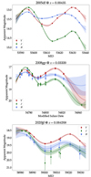 |
Fig. 1. PISCOLA light-curve (YJH-bands) fits of three SNe Ia: 2005df (Literature; top), 2008gp (CSP; middle), and 2020jjf (DEHVILS; bottom). The photometric uncertainties propagates into the fits themselves. |
5. Near-infrared light-curve decomposition
Principal component analysis (PCA; Pearson 1901; Hotelling 1933) is a statistical technique for linear transformation of a set of basis functions into a new coordinate system. The new basis functions are sorted in terms of the degree to which they describe the variance in the original data. Although PCA is commonly used for dimensionality reduction, it has several different applications depending on the goal. In the field of supernovae, PCA has been used in many different studies (e.g., Cormier & Davis 2011; Galbany 2014; Ishida et al. 2014; He et al. 2018; Shahbandeh et al. 2022; Holmbo et al. 2023; Lu et al. 2023; Burrow et al. 2024). In this work, PCA is used to produce a qualitative analysis of SNe Ia NIR light curves.
5.1. Light-curve preprocessing
Before applying PCA, a series of steps need to be performed for producing a sensible analysis. First, as PISCOLA fits do not rely on templates, we visually inspected the rest-frame light curves to make sure they are well-sampled and have physically expected shapes (i.e., two distinct peaks and a relatively smooth shape). This step mainly allows us to avoid including any noise in the decomposition. Primarily, SNe were removed due to relatively poor fit quality (e.g. due to large data uncertainty) or partial coverage of the light curves (2006D, 2008hy, 2008O, 2020kqv, 2020krw, 2020mby, 2020mdd, 2020tfc, and 2021glz). Additionally, SNe 2006le and 2009Y were removed only from the H-band light-curve analysis due to poor fit quality as well. SNe 2006X and 2020mvp were removed due to high host extinction, as suggested by the high E(B−V)host values (1.357 and 0.792 mag, respectively) obtained with SNooPy fits to the SN Ia sample, using the EBV_model2 model3. In particular, SN 2006X was already known to have high reddening (e.g., Wang et al. 2008; Folatelli et al. 2010). Another SN removed is 2020mbf, identified as a peculiar sub-type in this work. This object shows relatively flat NIR light curves, even in the J band, with a very shallow valley, which hints toward a 06bt-like SN (Foley et al. 2010). The light curve and PISCOLA fit of this SN can be found in Fig. A.1. SN 2008hs is also identified as a peculiar sub-type and removed given that this object presents a secondary NIR peak happening at much earlier phase compared to the rest of the sample, hinting toward a possible transitional SN Ia (see Fig. A.1 as well). We note, however, that this SN has not been classified as such and it even passes the color-stretch cut applied below. Additionally, as PCA does not propagate uncertainties, we only selected SNe with relatively small photometric uncertainties (σm). We chose those with σm < 0.2 mag across the entire phase range used (see below). Although applying a lower uncertainty threshold grants more precision, it also reduces the sample size, which is already very limited. We then used the color-stretch parameter, sBV4 (Burns et al. 2014) to remove the SNe falling outside the “normal” expected range (i.e., those with 0.6 ≤ sBV ≤ 1.4). SNe 2007on, LSQ12fvl, and 2020uea did not pass this last cut, given their lower values.
To summarize, from the initial sample of 158 SNe Ia, and after removing those with bad fits, peculiar shapes, relatively large uncertainties, and sBV outside the adopted range, only 47, 36, and 25 SNe remained for the YJH bands, respectively. The cuts applied in this section are presented in Table 2.
After these cuts, the NIR light curves were shifted in time to match at the epoch of B-band maximum luminosity, as obtained with SNooPy using the max_model model. We then selected the light curve range between –8 and +34 days with respect to the B-band peak, for each band independently. This somewhat arbitrary range approximately covers the first NIR peak, which happens at ∼5 days before optical peak and extends to the secondary peak, which occurs after 20 days (see Fig. 2; Dhawan et al. 2015).
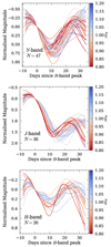 |
Fig. 2. SNe Ia rest-frame light curves after the preprocessing steps of Sect. 5.1. The phase range covers from −8 to +34 days with respect to optical peak. The light curves are color-coded by sBV value, obtained with SNooPy fits using the max_model model, limiting the color range between 0.8 ≤ sBV ≤ 1.2 for visualization purposes, as the bulk of the sample falls within this range. |
The last step of this process is normalizing the light curves by the brightness at the time of B-band peak. This prevents the global scale from dominating the sample variance and allows the PCA decomposition to focus on other light curve features instead. Additionally, this removes the dependence on distance, which is not normally known with high accuracy for these extragalactic transients.
Figure 2 shows the YJH-band light curves of SNe Ia after the aforementioned prepossessing steps. In the case of the J and H bands, around one third of the SNe come from CSP and one third from the literature, while for the Y band, around 50% come from CSP, one third from DEHVILS, and a small handful of objects from the literature. In general, a similar trend is observed for the YJH-band light curves, where the SNe with lower sBV values have earlier secondary peaks compared to those with higher values, following the same behavior described by Phillips (2012) (see also Sect. 6.3.2).
In terms of limitations and caveats, it is worth noting that the samples used are very limited in number. Given the requirements, the samples are mostly biased toward very nearby SNe (z ≲ 0.04, with only a few SNe, mostly from DEHVILS, between 0.04 < z ≲ 0.08) and most likely bright events. However, at low redshifts K-corrections are expected to be small. Although the samples for the different bands have different number of SNe, we note that their sBV distributions are approximately consistent, with most SNe within the 0.8 < sBV < 1.2 range.
5.2. Light-curve decomposition
In Fig. 3, we show the YJH-band light curves (top, middle, and bottom rows, respectively) decomposed into three PCA components. The first component (left column) captures most of the contribution to the light-curve variability (∼45 − 55%), while the second one (middle column) has moderate contribution (∼25 − 35%), and the third component (right column) mainly captures the remaining diversity (10%), although it could also have contribution from noise within the data. In total, two PCA components explain around 80% of the variability for each NIR band, while three components explain 90%, demonstrating their homogeneity.
 |
Fig. 3. PCA decomposition for the Y- (top row), J- (middle row), and H-band (bottom row) light curves. Color-coded are the contributions of each of the coefficients with a 2σ range: p0 (left column), p1 (middle column), and p2 (right column). The sample mean is shown as a solid red line. The values in parentheses are the percentages of the explained variance. Three components explain ∼90% of the variance for each of the bands. |
Following the PCA decomposition, for each band X, the light curve can be described by
 (1)
(1)
where  is the light-curve mean for the sample (solid red line in Fig. 3), and the three (N = 3) components (Ci) are in common for the entire sample used, while the coefficients (pi) depend on each SN. In the following section, we analyze what each of these components represents, how they contribute to the NIR light-curve shape, and we look for correlations with other parameters.
6. Analysis
In the previous section, the NIR light curves were decomposed using PCA. As a reminder to the reader, the PCA components (Ci) are orthogonal, providing different but complementary information. This section provides a detailed discussion of these components.
6.1. PCA components contribution to the NIR light curves
As can be seen from Fig. 3, the first PCA component (C0) encompasses around half of the explained variance for each of the bands, while C0 behaves in a similar way for the J and H bands; that is, it mainly describes how early or late the local minima and secondary peaks occur, with some contribution to the secondary peak brightness. For the Y band, C0 mainly controls the depth of the local minimum, including contribution to the timing of the secondary peak as well, but with a somewhat opposite effect compared to the other two bands. This difference between the bands might be surprising as we would expect the NIR light curve to behave in a similar manner. However, the physical processes that each wavelength range probes can differ (see more details below).
Examining the second PCA component (C1) reveals its primary contribution to the brightness of the secondary peak across all bands, along with some influence on the timing of the secondary peak in the Y and H bands. However, it also controls the depth of the local minima for the J and H bands, and the brightness of the first peak for the H band. It is also worth noting that the variability around first peak captured by the PCA on the Y and J bands is relatively small, but not so much for the H band, which could be due to a wider range in the phase of the first NIR peak found at this latter band (Dhawan et al. 2015). We also find a moderate correlation between C1 from the Y band and C0 from the J and H bands. Additionally, C1 from the H band is especially similar to C0 from the Y band (see Fig. 3). This shows that the different components trace similar behavior for all the NIR bands, but with different relative importance.
As the third PCA component (C2) only contributes to ≲10% of the variance in all bands and as it could be capturing noise in the data, we refrain from any interpretations and do not consider it in the rest of the analysis. To summarize, both C0 and C1 components mainly describe the timing and prominence of the secondary peak, but with somewhat opposite effects. Henceforth, we refer to the PCA components (Ci) and coefficients (pi) interchangeably.
6.2. Physical interpretation of the PCA components
Interpreting PCA components presents a challenge due to the complexity of the underlying physics governing NIR light curves, where multiple physical processes are intertwined. K06 provided one of the few most recent detailed theoretical models of SNe Ia NIR light curves available, serving as the primary reference for this study. In particular, K06 used radiative transfer calculations, assuming local thermodynamic equilibrium (LTE), to calculate the optical and NIR light curves of SNe Ia, produced by Chandrasekhar-mass WDs. They also studied the effect of three main physical properties on the secondary NIR peak: the mixing of 56Ni, the mass of 56Ni (MNi), and the mass of stable iron-group elements (MFe) produced by electron-capture elements and as a consequence of progenitor metallicity. These properties are detailed below.
-
Mixing: the mixing of iron-group elements, in particular 56Ni, into the outer layers of the ejecta hastens the occurrence of the secondary peak by increasing the extent of the iron core. Thus, more mixing translates into an earlier secondary peak as the recombination of iron-group elements (Fe III → Fe II) happens at earlier epochs.
-
MNi: this parameter has two opposing effects. On the one hand, a larger MNi implies a larger iron core, hastening the appearance of the recombination of iron-group elements. On the other hand, a larger MNi implies higher temperatures, which means that the recombination temperature is reached at later epochs as it takes longer to cool down. K06 showed that the latter effect dominates over the former one.
-
MFe: although SN Ia explosions primarily produce radioactive 56Ni, some non-negligible fraction of stable iron-group elements can be produced. The larger the amount of MFe produced by electron-capture elements (e.g., 57Co, 58Ni, 54Fe), the larger the size of the iron core, hastening the occurrence and increasing the prominence of the secondary peak. The progenitor metallicity also plays an important role in the production of stable iron-group elements. When MFe is produced at expense of MNi, lower temperatures are reached, producing an earlier and somewhat fainter secondary peak.
The variability captured by C0 for the J and H bands is dominated by the timing of the secondary peak, with some degree of dependence on its brightness (see Fig. 3). From the physical properties studied by K06, MNi and metallicity produce a similar behavior as observed for this component, where SNe Ia with later secondary peaks are also brighter. Ashall et al. (2019a,b) showed that the blue-edge velocity of the Fe/Co/Ni emission feature in the H-band, measured between a week or two after optical maximum, traces the outer 56Ni layer, which could potentially be used as a way of disentangling the effects of MNi and metallicity. However, to see whether one effect does indeed dominate over the other, a more detailed analysis of physical properties is needed (see Sect. 6.3).
In the J band, C1 primarily captures to the relative brightness (see Fig. 3), with a very small effect on the timing of the secondary peak. The physical properties studied by K06 predominantly affect the timing of the secondary peak, so in order to reproduce the observed behavior, a combination of these with opposing effects on the timing would be required. For instance, a mixture of MNi and MFe produced from electron-capture elements, or 56Ni mixing, would affect the brightness and leave the timing of the secondary peak relatively unaffected. For the H-band C1 component (see Fig. 3), both the 56Ni mixing and MFe produced from electron-capture elements could explain the observed behavior; especially the latter property, which has a greater effect on the secondary peak brightness.
Although K06 did not model the Y-band light curve, the analysis of both the I and J bands can be used as an approximation. The Y-band C0 component resembles the C1 component of the H band, and vice-versa (see Fig. 3), which would suggest that the same physical properties dominate these components. In other words, the same physical properties behind C1 and C0 for the H band could explain the behavior of C0 and C1, for the Y band. Certain physical properties, such as opacity and energy distribution, influence the SEDs of SNe Ia in varying ways across different wavelengths, possibly explaining why some physical properties would be dominant in one band and some in others. In addition, different NIR wavelengths probe different layers within the ejecta (and more deeply than the optical) at the same epoch (Wheeler et al. 1998), which is also a viable explanation.
The analysis of spectral features can also be used to help explain the difference in variability between different wavelength ranges. As spectroscopic observations at NIR wavelengths are relatively limited, theoretical models provide an excellent alternative. Collins et al. (2022) presented 3D radiative transfer simulations of double-detonation sub-Chandrasekhar-mass WDs as a plausible scenario of SN Ia explosions. These simulations show that the NIR spectra of SNe Ia around the time of secondary NIR peak are dominated by iron-group elements5. This is in good agreement with previous theoretical works (e.g., K06) and observations (e.g., Marion et al. 2003, 2009). In particular, the Y band (λ ∼ 1.0 μm) is dominated by Fe II, followed by Co II; H band (λ ∼ 1.6 μm) is dominated by Co II, followed by Fe II; while the J band (λ ∼ 1.2 μm) has a relatively similar contribution from Fe II, Co II, and Ca II. This is in agreement with observations, except for the J band, where not much Co II is observed and where Ca II is just observed around the optical peak (Marion et al. 2003, 2009). Nonetheless, this shows that despite their apparent similarity, the NIR bands have intrinsic differences as well, thus probing different aspects of the explosion. The opposite relative contribution from Fe II and Co II to the Y and H bands could possibly explain the relation between the C0 and C1 components seen for these bands (see Fig. 3). However, one caveat related these simulations is that they are not fully non-LTE (Collins et al. 2022), which tends to produce less realistic results.
To summarize, the JH-band C0 and Y-band C1 components seem to mainly trace the effect of MNi and metallicity on the secondary NIR peak, while the JH-band C1 and Y-band C0 components could capture the effect of 56Ni mixing and MFe. Additionally, some of the differences between the bands may be attributed to the different ejecta layers they trace. In the next section, we explore correlations between light-curve parameters and PCA components to help disentangle the effects of different physical properties.
6.3. Comparison to light-curve parameters
To have a better understanding about the physics behind each of the PCA components, we proceeded to compare them against different light-curve parameters. We calculated the linear relation for each pair of parameters, by using the Pearson correlation coefficient (ρ) and p-value. The values of ρ range from −1, completely anti-correlated, to 1, completely correlated, where 0 is no correlation. The p-value gives the probability of the null hypothesis (slope of the linear relation being equal to zero) being true. Commonly, if the p-value is below 0.05, the null hypothesis is discarded. We used Monte-Carlo sampling (1000 realizations) from the light-curve parameters and their respective uncertainties to propagate the errors into ρ and the p-value. We assume no uncertainty for the PCA coefficients (p0 and p1) as PCA does not propagate the uncertainty.
6.3.1. NIR peak absolute magnitude
In the top and bottom panels of Fig. 4, relations between the NIR peak absolute magnitudes6 and the first two PCA components (p0 and p1) are presented. No correlations are found for the J7 and H bands, although the Y band shows a significant but relatively weak correlation. If SNe Ia were to be standardizable candles in the NIR, correlations could be expected between their peak brightness and other light-curve parameters, which is not what the J and H band show. However, the Y band, which closer to the optical wavelengths than the other two bands, does show some correlation. The standardization of the Y band is studied in Sect. 6.6.
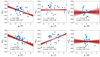 |
Fig. 4. Comparison of the first (p0; top row) and second (p1; bottom row) PCA coefficients vs. the peak absolute magnitude for each NIR band. The Pearson correlation coefficient (ρ) and p-value for each of the comparisons, with their respective 1σ uncertainty estimated by Monte-Carlo sampling, are shown with the respective linear relations (red lines). The null-hypothesis is that there is no correlation (zero slope). The panels have the same x- and y-axis ranges for visualization purposes. |
6.3.2. Color-stretch, sBV
In the top panels of Fig. 5, we show the relation between p0 and sBV for each of the NIR bands. sBV works as a tracer of the time when the iron-group elements recombine (Fe III → Fe II; appendix of Galbany et al. 2023). If this were true, we would expect very strong correlations between these parameters. Indeed, it can be seen that both J and H bands show strong correlations between sBV and p0, but the Y band does not. However, the latter shows a strong correlation between sBV and p1, while the other two bands do not (see bottom panels of Fig. 5). As sBV correlates with MNi, this is evidence in favor of our interpretation in Sect. 6.2. Additionally, Lu et al. (2023) already showed that sBV can successfully capture the NIR light-curve shape of SNe Ia. However, it is worth noting that this parameter is not correlated with all PCA components, so the NIR variability may be more complex than we could expect. One caveat in this comparison is that the SNooPy NIR templates, used for correcting the light curves (Sect. 4), are based on the sBV parameter; thus, a completely independent comparison is not possible as the PCA and sBV are linked from the start.
6.3.3. Optical peak absolute magnitude
It is known that the light curves of SNe Ia are primarily powered by the decay of 56Ni (Colgate & McKee 1969). Hence, their peak bolometric brightness is proportional to the MNi produced in the explosion (known as Arnett’s rule; Arnett 1982). As most of the luminosity (∼85%) of SNe Ia is emitted at optical wavelengths (Maguire 2017), the optical luminosity at its peak can be used as a proxy for MNi (e.g., Stritzinger et al. 2006). We found a correlation between the optical peak absolute magnitudes (BV bands) and p1 for the Y band and p0 for the J band. This is shown in Fig. 6. These correlation aligns with our analysis from Sect. 6.2, where C1 describes the contribution of MNi for the Y band and C0 for the J band, although no correlation was found for the H band. It is possible that MNi could have less influence toward redder wavelengths given the diminishing strength and significance of the correlation from Y to H.
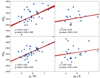 |
Fig. 6. Comparison between B- (top panels) and V-band (bottom panels) peak absolute magnitudes versus p1 for the Y band (left panels) and p0 for the J band (right panels). |
6.4. Comparison to host-galaxy properties
It has been known for over a decade that the environment in which SNe Ia reside affects their peak optical brightness, where SNe in more massive environments are brighter, on average, compared to those in less massive hosts, after standardization (e.g., Kelly et al. 2010; Lampeitl et al. 2010; Sullivan et al. 2010). However, whether this dependence is mainly due to external factors, such as dust (Brout & Scolnic 2021), or other intrinsic effects (e.g., Ginolin et al. 2025), is still a matter of debate.
Overall, NIR observations of SNe Ia can provide clues on this matter as these wavelengths are less affected by dust extinction. In fact, it has already been shown in recent years that the NIR peak brightness of SNe Ia does depend on the environment in which they reside (e.g., Uddin et al. 2020, 2024; Ponder et al. 2021), most likely implying that dust is not the dominant mechanism behind this relation. However, to our knowledge, the effect of the environment on the NIR light curves beyond first peak has not been explored yet and this approach could provide new insights into the physics of these transients.
In this work, we used previous estimates of the host-galaxy masses from the literature. Uddin et al. (2024) provides host-galaxy masses for the entire CSP sample (CSP-I and CSP-II), which represents a large fraction of the samples used (see Sect. 5.1). In addition, Ponder et al. (2021) estimated host-galaxy masses for several SNe from different surveys and others from the literature. Although they also included CSP-I, we prioritized the values from Uddin et al. (2024) for consistency. Finally, Peterson et al. (2024) provided values for the DEHVILS sample8. Although different studies estimate host masses with different methods, they usually agree relatively well.
In Fig. 7, the relation between host-galaxy stellar mass, log10(M/M⊙), and p0 is shown. Although no correlation is found, a possible lack of SNe with faint J-band secondary peak in low-mass hosts is apparent. However, this could be due to a bias given the relatively small number of SNe in the sample. Additionally, no clear trend was found with p1, possibly implying that the environment has no visible effect on the secondary NIR peak of SNe Ia; however, no strong conclusions can be drawn. We do note that the host-galaxy mass, while easier to estimate than other host properties, might not adequately capture the effect of the environment on SNe Ia NIR light curves.
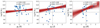 |
Fig. 7. Comparison between host-galaxy stellar mass, log10(M/M⊙) and p0. The vertical dashed line marks p0 = 0.0, dividing the SN Ia sample at the mean, while the horizontal lines mark log10(M/M⊙) = 10, commonly used for splitting SNe Ia samples into high- and low-mass hosts. |
The relation between host-galaxy color excess, E(B−V)host (obtained with SNooPy using the EBV_model2), and the first two PCA components has been here studied as well. As with log10(M/M⊙), we did not find any clear correlation. Assuming that dustier galaxies are expected to be more metal-rich (i.e., with more metal-rich progenitors), some correlation would be expected given our analysis in Sect. 6.2, but a more precise estimation of metallicity would be needed to draw any strong conclusions. Future works will extend to the use of other galaxy properties, such as the star formation rate and metallicity, to further study the impact of the environment on the secondary NIR peak of SNe Ia.
6.5. NIR color-curves decomposition
Following the PCA decomposition of the NIR light curves of SNe Ia, we studied the decomposition of the rest-frame, K- and MW-corrected, NIR color curves: (Y − J), (Y − H), and (J − H). The same criteria applied in Sect. 5.1 were applied here, except for the normalization in the y-axis. The color curves are shown in Fig. 8. We note that the number of SNe Ia used in this case is reduced compared to those in Sect. 5, due to the requirements of having two bands with proper coverage instead of one. An inspection of Fig. 8 reveals that the (Y − J) and (J − H) color curves follow a very similar evolution to those shown by Lu et al. (2023), where there is a clear separation between SNe Ia with high and low sBV. This means that SNe Ia that are optically bluer around optical maximum have on average redder NIR colors around the time of secondary NIR peak. However, the NIR color as a function of sBV does not present a monotonic transition as smooth as that seen in Lu et al. (2023).
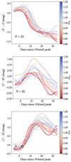 |
Fig. 8. Same as Fig. 2, but for the color-curves: (Y-J) (top panel), (Y-H) (middle panel), and (J-H) (bottom panel). |
The color-curve decomposition is presented in Fig. 9. It can be noted that the first component (C0) captures over 50% of the variance for all color curves, while relatively low variance is captured by the other components. Additionally, it can be seen that NIR color curves present relatively high intrinsic uniformity around optical peak, also shown in Fig. 8.
The C0 components mainly capture how blue or red the NIR color curves are, where SNe with higher NIR colors peak at later epochs (see Fig. 9). Additionally, sBV seems to trace the same behavior as C0 (see Fig. 8). It can also be seen that the NIR color curves of SNe Ia show some similarity in evolution with the (B − V) curve, but reach their reddest point at much earlier phases: around 5 days for (Y − J), 12 days for (Y − H), and 18 days for (J − H). In other words, p0 could be linked to an sBV-like parameter in the NIR and trace similar information. For instance, the peak in the (J − H) curve approximately coincides with the local minimum on the J band (see Figs. 3 and 9), possibly tracing the onset of the recombination of iron-group elements.
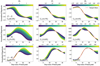 |
Fig. 9. Same as Fig. 3, but for PCA decomposition of the SNe Ia color curves: (Y-J) (top row), (Y-H) (middle row), and (J-H) (bottom row). |
When comparing the PCA components against NIR peak absolute magnitude, we see no clear correlations, except for the (Y − H) C1 components. However, the variance explained by this component is relatively low (∼14%), so it does not carry much information. This lack of correlation is not surprising as similar results were found in general for the decomposition in Sect. 6.3.1.
In Fig. 10, we see a clear correlation between sBV and p0 for all the NIR colors. Again, this is not surprising given the NIR templates from Lu et al. (2023) were built as a function of sBV. However, the scatter shows the complexity of NIR variability, which cannot be entirely captured by a single parameter.
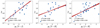 |
Fig. 10. sBV vs. PCA p0 coefficient for the NIR color curves. |
In the case of the peak absolute magnitude at optical wavelengths (both B and V bands), we see correlations with p0 for all the NIR color curves (see Fig. 11). This is in line with the correlations found with sBV and shows that SNe Ia with more MNi have redder NIR colors.
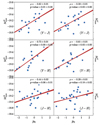 |
Fig. 11. B-band (left panels) and V-band (right panels) peak absolute magnitude vs. PCA p0 coefficient for the NIR color curves. |
The comparison against host properties presents some interesting results as well. In the top panel of Fig. 12, the correlation between log10(M/M⊙) and p0 for the different color curves is shown. Although these correlations can be driven by a bias due to the small sample of SNe Ia, the same trend is observed for all color curves, where the redder objects are preferentially found in less massive galaxies (see Fig. 12). If this were true (and assuming that more massive galaxies are also more metal rich), this results would align with the expected effect of metallicity on the secondary NIR peak (Fig. 13 in K06), where the more metal-poor objects would have redder NIR colors and vice versa. However, a larger sample would be needed to confirm this.
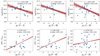 |
Fig. 12. Comparison between log10(M/M⊙) (top panels) and E(B−V)host (bottom panels) vs. p0 for the NIR colors. |
When the same comparison is made against E(B−V)host (bottom panel of Fig. 12), we see correlations for the C0 component of (Y − J) and (Y − H). These are mainly driven by a couple of SNe (top right points in the bottom left and middle plots of Fig. 12): 2007ca and 2008fp, both from the CSP survey. A close inspection to the light-curve fits does not reveal any abnormality. When comparing to another SN with similar p0 but lower E(B−V)host, SN 2017cbv, these SNe show higher (i.e., redder) (B − V)∼, (Ymax − Jmax) and (Bmax − Jmax) values. When comparing to a SN with a similarly high E(B−V)host but lower p0, 2007le, the only difference is that the latter has a bluer Bmax − Jmax value. Whether there is a potential bias in the estimation of E(B−V)host is hard to tell, but the comparison between SNe, coupled with the fact that no correlation is seen between C0 and (J − H), possibly suggests that the correlations found might be driven by the relatively low statistics.
As K06 did not provide models for the color curves and no model for the Y band, it is challenging to obtain more insights into the physical interpretation of these PCA components.
6.6. NIR light-curve standardization
Following the correlation found between Y-band peak absolute magnitude (MY) and the PCA components (see Sect. 6.3.1), we proceeded to test the standardization of the Y-band light curves of SNe Ia by adding correction parameters for the estimation of distances, expressed as
 (2)
(2)
where mY is the Y-band peak apparent magnitude, and α and β are nuisance parameters. We followed a similar procedure as in Galbany et al. (2023), but fixed H0 = 70 km s−1 Mpc−1 and fit for M and σint (SN intrinsic scatter), with the addition of α and β. Since H0 is fixed, distances from the calibrating SNe are not needed to anchor the y-axis in the Hubble diagram to break the degeneracy between H0 and M.
Figure 13 shows the corner plot of the Markov chain Monte Carlo (MCMC) posterior distributions of the fitted parameters used for building the Y-band Hubble diagram with standardization (Fig. 14). The addition of standardization parameters is favored by around 3σ and 2σ significance for p0 and p1, respectively. Additionally, by correcting the light curves, σint is reduced from 0.21 mag to 0.17 mag. Although the quoted values might seem high at first, this is mainly attributed to the lack of uber-calibration of the photometry required for a precise cosmological analysis, which is beyond the scope of this work9. The peculiar velocities of low-z SNe Ia also affect the measured scatter, but removing these objects would further reduce the sample size.
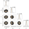 |
Fig. 13. Corner plot of the MCMC posterior distributions used for building a Y-band Hubble diagram. σint is the intrinsic scatter, i.e., leftover scatter unexplained by the standardization. The solid lines show the mean of the distributions while the dashed lines show the 16th and 84th percentiles (1σ). |
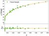 |
Fig. 14. Y-band Hubble diagram with the standardization from Fig. 13. The solid line represents the fitted cosmology, a flat ΛCDM cosmological model with Ωm = 0.3 and H0 = 70 km s−1 Mpc−1. The Hubble residual presents a RMS of 0.27 mag and a normalised median absolute deviation of 0.10 mag. |
While the standardization in the Y band is favored, the J and H bands do not present any improvements with the addition of other parameters, reflecting their uniformity. The standardization using the PCA components from the NIR color curves is covered in Appendix B.
7. Summary and conclusions
In this work, we gathered a sample of 47, 36, and 25 SNe Ia with well-sampled YJH-band light curves, respectively, to analyze their variability with PCA, a common machine-learning technique. SNe Ia were selected from various sources, including the CSP, CfAIR2, RATIR, and DEHVILS surveys, as well as some objects drawn from the literature. Each selected object has at least five NIR photometric epochs in any band, with coverage spanning from the first to the second peak. The light curves were corrected for K-correction and Milky Way extinction using SNooPy, then interpolated with PISCOLA to achieve continuous rest-frame coverage.
Decomposing the NIR light curves, each one independently and using three PCA components (C0, C1, and C2) explains ∼90% of the variability, with the first component explaining around 50% of it. The C0 component of the J and H bands (C1 for the Y band) shows that brighter secondary peaks also occur at later epochs and vice versa. With a somewhat opposing effect, the C1 component of the H band (C0 for the Y band) shows that brighter secondary peaks occur at earlier epochs, while this component mainly just contributes to the brightness for the J band. A possible explanation for the NIR bands exhibiting different dominant behaviors is that the PCA components could be tracing different physical properties, such as the effect of MNi, metallicity, or MFe on the time of recombination of iron-group elements and, subsequently, on the secondary peak. When comparing to observations and theoretical models, a difference in the elements abundance is seen for the different wavelengths ranges each of the bands probes, possibly explaining some of the differences seen with the PCA components.
When comparing the PCA coefficients (p0 and p1) against different light-curve parameters, some interesting trends are found. The NIR peak absolute magnitude correlates with p0 for the Y band, which could imply some correlation between secondary peak brightness and MNi. However, the same correlations are not seen for the J and H bands. Nonetheless, the optical peak brightness, which can be used as a proxy for MNi, correlates with p1 for the Y band and p0 for the J band, suggesting a possible diminishing influence of MNi in the secondary peak toward redder wavelengths.
We also compared the PCA coefficients against host-galaxy properties, in particular, stellar mass and color excess, but we found no clear correlations. However, we cannot say whether the environment does not affect the secondary NIR peak. A larger sample and, in particular, a comparison with other host-galaxy properties, such as the star formation rate and metallicity, would be needed to draw a strong conclusion in this regard.
The PCA decomposition was also applied on the NIR color curves of the SNe Ia, where over 50% of the variance is explained by the first component (C0). Although the physical interpretation of these is more complex, we still compared them against light-curve properties. We found correlations between the C0 component and peak optical brightness (i.e., MNi) for all the NIR colors, showing that SNe with larger amounts of MNi have redder NIR colors. When comparing to the same host properties as before, we found a tentative correlation with log10(M/M⊙), where SNe Ia with redder NIR colors are found on less massive galaxies (potentially more metal-poor) environments. The comparison against E(B−V)host shows some correlations, but mainly driven by two SNe and possibly due to the relatively low statistics.
Given the correlation found between MY and p0, we tested the standardization of the Y-band light curves, finding a reduction in σint of 0.04 mag when correcting the Y-band luminosity. Future research will allow us to investigate whether applying corrections at these wavelengths offers a genuine advantage, given the need for good photometric coverage, compared to using a single NIR epoch (Stanishev et al. 2018; Müller-Bravo et al. 2022a), which benefits from increasing the statistical sample size of SNe Ia. The Vera C. Rubin Observatory Legacy Survey of Space and Time (Ivezić et al. 2019) will provide y-band photometry for SNe, which can be used as a test set.
NIR observations of SNe Ia provide a unique opportunity to study the physics of these transients and for doing cosmology. Although the number of objects observed in the NIR has been steadily increasing in the last decade, there is still a very limited number of these with high-cadence observations covering both NIR peaks. Surveys such as CSP present unique datasets to study these transients in detail given the rich photometric and spectroscopic coverage. Photometry from new low- and high-redshift surveys, such as the Aarhus-Barcelona FLOWS project10, Hawai’i Supernova Flows (Do et al. 2025), and JADES (DeCoursey et al. 2025), will further increase the numbers. This will be essential for making the most of future observations from Euclid and the Roman Space Telescope.
Finally, we would like to encourage the community to produce new and more sophisticated theoretical models of SNe Ia extending to NIR wavelengths. These models can be used to make comparisons against the increasing amount of data, helping constrain their physics and improve their usefulness as cosmological distance indicators.
Data availability
Most data used in this work form part of published articles. Published data can be shared upon request to the authors. Private data from CSP-II will be published in an upcoming article (Suntzeff et al., in prep.).
For an expanding ejecta, the flux is proportional to TRphot, where T is the temperature and Rphot is the radius of the photosphere.
AB to Vega offsets of 0.894 and 1.368 mag in J and H bands are applied, respectively. We did not find any published AB to Vega offset value for the Y band, so we follow the notes in https://ratir.astroscu.unam.mx/instrument.html and apply an offset of 0.634 mag as described in Table 7 of Hewett et al. (2006), which is only an approximation.
This model has tmax, the distance modulus (μ) and E(B−V)host as free parameters.
This parameter measures the stretch in the (B − V) color curve that peaks around 30 days after optical maximum, combining the stretch and color parameters into a single one.
Christine Collins (private communication).
Assuming a cosmology with Ωm = 0.3, Ωλ = 0.7 and H0 = 70 km s−1 Mpc−1.
The correlation for p1 in the J band is driven by a single data point, at the bottom left.
Erik Peterson was kind enough to share with us the host-galaxy masses, including uncertainties, estimated with Prospector (Leja et al. 2017; Johnson et al. 2021), as those in Peterson et al. (2024) do not include these uncertainties.
We note that restricting the sample to a single survey, such as CSP, largely reduces the scatter, but limits the sample size.
Acknowledgments
The authors thank the anonymous referee for a constructive review that has improved the quality and content of this publication. T.E.M.B. would like to thank Kate Maguire for very insightful discussions about the physical interpretation of the PCA components for the analysis. T.E.M.B. and L.G. acknowledge financial support from the Spanish Ministerio de Ciencia e Innovación (MCIN), the Agencia Estatal de Investigación (AEI) 10.13039/501100011033, the European Social Fund (ESF) “Investing in your future, and the European Union Next Generation EU/PRTR funds under PID2020-115253GA-I00 HOSTFLOWS and PID2023-151307NB-I00 SNNEXT projects, the 2021 Juan de la Cierva program FJC2021-047124-I, and from Centro Superior de Investigaciones Científicas (CSIC) under PIE 20215AT016, ILINK23001, COOPB2304 projects, and the program Unidad de Excelencia María de Maeztu CEX2020-001058-M. T.E.M.B. is funded by Horizon Europe ERC grant no. 101125877. M.D.S. and the FLOWS project is funded by the Independent Research Fund Denmark (IRFD, grant number 10.46540/2032-00022B) and by the Aarhus University Research Foundation (Nova grant 44369). The work of the Carnegie Supernova Project has been supported by the NSF under the grants AST0306969, AST0607438, AST1008343, AST1613426, AST1613472 and AST613455. Software: astropy (Astropy Collaboration 2013, 2018), corner (Foreman-Mackey 2016), emcee (Foreman-Mackey et al. 2013), extinction (Barbary 2016), matplotlib (Hunter 2007), numpy (Harris et al. 2020), pandas (McKinney 2010), peakutils (Negri & Vestri 2017), PISCOLA (Müller-Bravo et al. 2022b), scikit-learn (Pedregosa et al. 2011), scipy (Virtanen et al. 2020), sfdmap (https://github.com/kbarbary/sfdmap), SNooPy (Burns et al. 2011), tinygp (Foreman-Mackey et al. 2024)
References
- Arnett, W. D. 1982, ApJ, 253, 785 [Google Scholar]
- Ashall, C., Hoeflich, P., Hsiao, E. Y., et al. 2019a, ApJ, 878, 86 [Google Scholar]
- Ashall, C., Hsiao, E. Y., Hoeflich, P., et al. 2019b, ApJ, 875, L14 [Google Scholar]
- Ashall, C., Lu, J., Burns, C., et al. 2020, ApJ, 895, L3 [NASA ADS] [CrossRef] [Google Scholar]
- Astropy Collaboration (Robitaille, T. P., et al.) 2013, A&A, 558, A33 [NASA ADS] [CrossRef] [EDP Sciences] [Google Scholar]
- Astropy Collaboration (Price-Whelan, A. M., et al.) 2018, AJ, 156, 123 [Google Scholar]
- Avelino, A., Friedman, A. S., Mandel, K. S., et al. 2019, ApJ, 887, 106 [Google Scholar]
- Barbary, K. 2016, https://doi.org/10.5281/zenodo.804967 [Google Scholar]
- Bellm, E. C., Kulkarni, S. R., Graham, M. J., et al. 2019, PASP, 131, 018002 [Google Scholar]
- Brout, D., & Scolnic, D. 2021, ApJ, 909, 26 [NASA ADS] [CrossRef] [Google Scholar]
- Burns, C. R., Stritzinger, M., Phillips, M. M., et al. 2011, AJ, 141, 19 [Google Scholar]
- Burns, C. R., Stritzinger, M., Phillips, M. M., et al. 2014, ApJ, 789, 32 [Google Scholar]
- Burrow, A., Baron, E., Burns, C. R., et al. 2024, ApJ, 967, 55 [Google Scholar]
- Cartier, R., Hamuy, M., Pignata, G., et al. 2014, ApJ, 789, 89 [NASA ADS] [CrossRef] [Google Scholar]
- Colgate, S. A., & McKee, C. 1969, ApJ, 157, 623 [NASA ADS] [CrossRef] [Google Scholar]
- Collins, C. E., Gronow, S., Sim, S. A., & Röpke, F. K. 2022, MNRAS, 517, 5289 [Google Scholar]
- Contreras, C., Hamuy, M., Phillips, M. M., et al. 2010, AJ, 139, 519 [Google Scholar]
- Cormier, D., & Davis, T. M. 2011, MNRAS, 410, 2137 [NASA ADS] [CrossRef] [Google Scholar]
- DeCoursey, C., Egami, E., Pierel, J. D. R., et al. 2025, ApJ, 979, 250 [Google Scholar]
- Dekany, R., Smith, R. M., Riddle, R., et al. 2020, PASP, 132, 038001 [NASA ADS] [CrossRef] [Google Scholar]
- Dhawan, S., Leibundgut, B., Spyromilio, J., & Maguire, K. 2015, MNRAS, 448, 1345 [NASA ADS] [CrossRef] [Google Scholar]
- Do, A., Shappee, B. J., Tonry, J. L., et al. 2025, MNRAS, 536, 624 [Google Scholar]
- Elias, J. H., Frogel, J. A., Hackwell, J. A., & Persson, S. E. 1981, ApJ, 251, L13 [NASA ADS] [CrossRef] [Google Scholar]
- Elias, J. H., Matthews, K., Neugebauer, G., & Persson, S. E. 1985, ApJ, 296, 379 [NASA ADS] [CrossRef] [Google Scholar]
- Elias-Rosa, N., Benetti, S., Cappellaro, E., et al. 2006, MNRAS, 369, 1880 [CrossRef] [Google Scholar]
- Elias-Rosa, N., Benetti, S., Turatto, M., et al. 2008, MNRAS, 384, 107 [Google Scholar]
- Folatelli, G., Phillips, M. M., Burns, C. R., et al. 2010, AJ, 139, 120 [Google Scholar]
- Foley, R. J., Narayan, G., Challis, P. J., et al. 2010, ApJ, 708, 1748 [NASA ADS] [CrossRef] [Google Scholar]
- Foley, R. J., Fox, O. D., McCully, C., et al. 2014, MNRAS, 443, 2887 [NASA ADS] [CrossRef] [Google Scholar]
- Foreman-Mackey, D. 2016, J. Open Source Softw., 1, 24 [Google Scholar]
- Foreman-Mackey, D., Hogg, D. W., Lang, D., & Goodman, J. 2013, PASP, 125, 306 [Google Scholar]
- Foreman-Mackey, D., Yu, W., Yadav, S., et al. 2024, https://doi.org/10.5281/zenodo.10463641 [Google Scholar]
- Förster, F., Cabrera-Vives, G., Castillo-Navarrete, E., et al. 2021, AJ, 161, 242 [CrossRef] [Google Scholar]
- Freedman, W. L., Burns, C. R., Phillips, M. M., et al. 2009, ApJ, 704, 1036 [Google Scholar]
- Friedman, A. S., Wood-Vasey, W. M., Marion, G. H., et al. 2015, ApJS, 220, 9 [NASA ADS] [CrossRef] [Google Scholar]
- Galbany, L. 2014, in Statistical Challenges in 21st Century Cosmology, eds. A. Heavens, J. L. Starck, & A. Krone-Martins, IAU Symposium, 306, 330 [Google Scholar]
- Galbany, L., de Jaeger, T., Riess, A. G., et al. 2023, A&A, 679, A95 [NASA ADS] [CrossRef] [EDP Sciences] [Google Scholar]
- Ginolin, M., Rigault, M., Copin, Y., et al. 2025, A&A, 694, A4 [NASA ADS] [CrossRef] [EDP Sciences] [Google Scholar]
- Graham, M. J., Kulkarni, S. R., Bellm, E. C., et al. 2019, PASP, 131, 078001 [Google Scholar]
- Grayling, M., & Popovic, B. 2025, MNRAS, 542, 2060 [Google Scholar]
- Hamuy, M., Folatelli, G., Morrell, N. I., et al. 2006, PASP, 118, 2 [NASA ADS] [CrossRef] [Google Scholar]
- Harris, C. R., Millman, K. J., van der Walt, S. J., et al. 2020, Nature, 585, 357 [NASA ADS] [CrossRef] [Google Scholar]
- He, S., Wang, L., & Huang, J. Z. 2018, ApJ, 857, 110 [Google Scholar]
- Hewett, P. C., Warren, S. J., Leggett, S. K., & Hodgkin, S. T. 2006, MNRAS, 367, 454 [Google Scholar]
- Hicken, M., Challis, P., Jha, S., et al. 2009, ApJ, 700, 331 [Google Scholar]
- Hicken, M., Challis, P., Kirshner, R. P., et al. 2012, ApJS, 200, 12 [Google Scholar]
- Hoeflich, P., Khokhlov, A. M., & Wheeler, J. C. 1995, ApJ, 444, 831 [CrossRef] [Google Scholar]
- Hoeflich, P., Hsiao, E. Y., Ashall, C., et al. 2017, ApJ, 846, 58 [Google Scholar]
- Holmbo, S., Stritzinger, M. D., Karamehmetoglu, E., et al. 2023, A&A, 675, A83 [NASA ADS] [CrossRef] [EDP Sciences] [Google Scholar]
- Hoogendam, W. B., Jones, D. O., Ashall, C., et al. 2025, Open J. Astrophys., 8, 120 [Google Scholar]
- Hotelling, H. 1933, J. Educ. Psychol., 24, 417 [CrossRef] [Google Scholar]
- Hsiao, E. Y., Conley, A., Howell, D. A., et al. 2007, ApJ, 663, 1187 [Google Scholar]
- Hsiao, E. Y., Marion, G. H., Phillips, M. M., et al. 2013, ApJ, 766, 72 [Google Scholar]
- Hsiao, E. Y., Burns, C. R., Contreras, C., et al. 2015, A&A, 578, A9 [NASA ADS] [CrossRef] [EDP Sciences] [Google Scholar]
- Hsiao, E. Y., Phillips, M. M., Marion, G. H., et al. 2019, PASP, 131, 014002 [NASA ADS] [CrossRef] [Google Scholar]
- Hunter, J. D. 2007, Comput. Sci. Eng., 9, 90 [NASA ADS] [CrossRef] [Google Scholar]
- Iben, I., Jr., & Tutukov, A. V. 1984, ApJS, 54, 335 [NASA ADS] [CrossRef] [Google Scholar]
- Ishida, E. E. O., Abdalla, F. B., & de Souza, R. S. 2014, in Statistical Challenges in 21st Century Cosmology, eds. A. Heavens, J. L. Starck, & A. Krone-Martins, IAU Symposium, 306, 326 [Google Scholar]
- Ivezić, Ž., Kahn, S. M., Tyson, J. A., et al. 2019, ApJ, 873, 111 [Google Scholar]
- Jha, S., Kirshner, R. P., Challis, P., et al. 2006, AJ, 131, 527 [Google Scholar]
- Johansson, J., Cenko, S. B., Fox, O. D., et al. 2021, ApJ, 923, 237 [NASA ADS] [CrossRef] [Google Scholar]
- Johnson, B. D., Leja, J., Conroy, C., & Speagle, J. S. 2021, ApJS, 254, 22 [NASA ADS] [CrossRef] [Google Scholar]
- Kasen, D. 2006, ApJ, 649, 939 [NASA ADS] [CrossRef] [Google Scholar]
- Kelly, P. L., Hicken, M., Burke, D. L., Mandel, K. S., & Kirshner, R. P. 2010, ApJ, 715, 743 [Google Scholar]
- Krisciunas, K., Suntzeff, N. B., Candia, P., et al. 2003, AJ, 125, 166 [NASA ADS] [CrossRef] [Google Scholar]
- Krisciunas, K., Phillips, M. M., & Suntzeff, N. B. 2004a, ApJ, 602, L81 [NASA ADS] [CrossRef] [Google Scholar]
- Krisciunas, K., Phillips, M. M., Suntzeff, N. B., et al. 2004b, AJ, 127, 1664 [NASA ADS] [CrossRef] [Google Scholar]
- Krisciunas, K., Suntzeff, N. B., Phillips, M. M., et al. 2004c, AJ, 128, 3034 [NASA ADS] [CrossRef] [Google Scholar]
- Krisciunas, K., Prieto, J. L., Garnavich, P. M., et al. 2006, AJ, 131, 1639 [Google Scholar]
- Krisciunas, K., Contreras, C., Burns, C. R., et al. 2017a, AJ, 154, 211 [NASA ADS] [CrossRef] [Google Scholar]
- Krisciunas, K., Suntzeff, N. B., Espinoza, J., et al. 2017b, Res. Notes Am. Astron. Soc., 1, 36 [Google Scholar]
- Lampeitl, H., Nichol, R. C., Seo, H. J., et al. 2010, MNRAS, 401, 2331 [NASA ADS] [CrossRef] [Google Scholar]
- Leja, J., Johnson, B. D., Conroy, C., van Dokkum, P. G., & Byler, N. 2017, ApJ, 837, 170 [NASA ADS] [CrossRef] [Google Scholar]
- Lu, J., Hsiao, E. Y., Phillips, M. M., et al. 2023, ApJ, 948, 27 [NASA ADS] [CrossRef] [Google Scholar]
- Maguire, K. 2017, in Handbook of Supernovae, eds. A. W. Alsabti, & P. Murdin, 293 [Google Scholar]
- Marion, G. H., Höflich, P., Vacca, W. D., & Wheeler, J. C. 2003, ApJ, 591, 316 [Google Scholar]
- Marion, G. H., Höflich, P., Gerardy, C. L., et al. 2009, AJ, 138, 727 [NASA ADS] [CrossRef] [Google Scholar]
- Marion, G. H., Sand, D. J., Hsiao, E. Y., et al. 2015, ApJ, 798, 39 [Google Scholar]
- Masci, F. J., Laher, R. R., Rusholme, B., et al. 2019, PASP, 131, 018003 [Google Scholar]
- Matheson, T., Joyce, R. R., Allen, L. E., et al. 2012, ApJ, 754, 19 [NASA ADS] [CrossRef] [Google Scholar]
- McKinney, W. 2010, in Proceedings of the 9th Python in Science Conference, eds. S. van der Walt, & J. Millman, 56 [Google Scholar]
- Meikle, W. P. S. 2000, MNRAS, 314, 782 [NASA ADS] [CrossRef] [Google Scholar]
- Miknaitis, G., Pignata, G., Rest, A., et al. 2007, ApJ, 666, 674 [NASA ADS] [CrossRef] [Google Scholar]
- Müller-Bravo, T. E., Galbany, L., Karamehmetoglu, E., et al. 2022a, A&A, 665, A123 [NASA ADS] [CrossRef] [EDP Sciences] [Google Scholar]
- Müller-Bravo, T. E., Sullivan, M., Smith, M., et al. 2022b, MNRAS, 512, 3266 [CrossRef] [Google Scholar]
- Negri, L. H., & Vestri, C. 2017, https://doi.org/10.5281/zenodo.887917 [Google Scholar]
- Nugent, P., Phillips, M., Baron, E., Branch, D., & Hauschildt, P. 1995, ApJ, 455, L147 [NASA ADS] [CrossRef] [Google Scholar]
- Nugent, P. E., Sullivan, M., Cenko, S. B., et al. 2011, Nature, 480, 344 [NASA ADS] [CrossRef] [Google Scholar]
- Oke, J. B., & Sandage, A. 1968, ApJ, 154, 21 [NASA ADS] [CrossRef] [Google Scholar]
- Pan, Y. C., Foley, R. J., Kromer, M., et al. 2015, MNRAS, 452, 4307 [CrossRef] [Google Scholar]
- Pearson, K. 1901, London Edinburgh Dublin Philos. Mag. J. Sci., 2, 559 [Google Scholar]
- Pedregosa, F., Varoquaux, G., Gramfort, A., et al. 2011, J. Mach. Learn. Res., 12, 2825 [Google Scholar]
- Pessi, P. J., Hsiao, E. Y., Folatelli, G., et al. 2022, MNRAS, 510, 4929 [NASA ADS] [CrossRef] [Google Scholar]
- Peterson, E. R., Jones, D. O., Scolnic, D., et al. 2023, MNRAS, 522, 2478 [NASA ADS] [CrossRef] [Google Scholar]
- Peterson, E. R., Scolnic, D., Jones, D. O., et al. 2024, A&A, 690, A56 [NASA ADS] [CrossRef] [EDP Sciences] [Google Scholar]
- Phillips, M. M. 1993, ApJ, 413, L105 [Google Scholar]
- Phillips, M. M. 2012, PASA, 29, 434 [NASA ADS] [CrossRef] [Google Scholar]
- Phillips, M. M., Krisciunas, K., Suntzeff, N. B., et al. 2006, AJ, 131, 2615 [Google Scholar]
- Phillips, M. M., Contreras, C., Hsiao, E. Y., et al. 2019, PASP, 131, 014001 [Google Scholar]
- Pignata, G., Benetti, S., Mazzali, P. A., et al. 2008, MNRAS, 388, 971 [NASA ADS] [CrossRef] [Google Scholar]
- Pinto, P. A., & Eastman, R. G. 2000, ApJ, 530, 757 [NASA ADS] [CrossRef] [Google Scholar]
- Ponder, K. A., Wood-Vasey, W. M., Weyant, A., et al. 2021, ApJ, 923, 197 [NASA ADS] [CrossRef] [Google Scholar]
- Pskovskii, I. P. 1977, Soviet Ast., 21, 675 [Google Scholar]
- Rasmussen, C. E., & Williams, C. K. I. 2006, Gaussian Processes for Machine Learning (The MIT Press) [Google Scholar]
- Riess, A. G., Kirshner, R. P., Schmidt, B. P., et al. 1999, AJ, 117, 707 [Google Scholar]
- Shahbandeh, M., Hsiao, E. Y., Ashall, C., et al. 2022, ApJ, 925, 175 [NASA ADS] [CrossRef] [Google Scholar]
- Srivastav, S., Ninan, J. P., Kumar, B., et al. 2016, MNRAS, 457, 1000 [Google Scholar]
- Stanishev, V., Goobar, A., Benetti, S., et al. 2007, A&A, 469, 645 [NASA ADS] [CrossRef] [EDP Sciences] [Google Scholar]
- Stanishev, V., Goobar, A., Amanullah, R., et al. 2018, A&A, 615, A45 [NASA ADS] [CrossRef] [EDP Sciences] [Google Scholar]
- Stritzinger, M., Leibundgut, B., Walch, S., & Contardo, G. 2006, A&A, 450, 241 [NASA ADS] [CrossRef] [EDP Sciences] [Google Scholar]
- Stritzinger, M. D., Phillips, M. M., Boldt, L. N., et al. 2011, AJ, 142, 156 [Google Scholar]
- Sullivan, M., Conley, A., Howell, D. A., et al. 2010, MNRAS, 406, 782 [NASA ADS] [Google Scholar]
- Tonry, J. L., Denneau, L., Heinze, A. N., et al. 2018, PASP, 130, 064505 [Google Scholar]
- Tripp, R. 1998, A&A, 331, 815 [NASA ADS] [Google Scholar]
- Uddin, S. A., Burns, C. R., Phillips, M. M., et al. 2020, ApJ, 901, 143 [NASA ADS] [CrossRef] [Google Scholar]
- Uddin, S. A., Burns, C. R., Phillips, M. M., et al. 2024, ApJ, 970, 72 [Google Scholar]
- Valentini, G., Di Carlo, E., Massi, F., et al. 2003, ApJ, 595, 779 [Google Scholar]
- Virtanen, P., Gommers, R., Oliphant, T. E., et al. 2020, Nat. Methods, 17, 261 [Google Scholar]
- Wang, X., Li, W., Filippenko, A. V., et al. 2008, ApJ, 675, 626 [NASA ADS] [CrossRef] [Google Scholar]
- Wang, L., Contreras, C., Hu, M., et al. 2020, ApJ, 904, 14 [NASA ADS] [CrossRef] [Google Scholar]
- Wee, J., Chakraborty, N., Wang, J., & Penprase, B. E. 2018, ApJ, 863, 90 [Google Scholar]
- Wheeler, J. C., Höflich, P., Harkness, R. P., & Spyromilio, J. 1998, ApJ, 496, 908 [Google Scholar]
- Whelan, J., & Iben, Icko 1973, J., ApJ, 186, 1007 [NASA ADS] [Google Scholar]
- Wood-Vasey, W. M., Friedman, A. S., Bloom, J. S., et al. 2008, ApJ, 689, 377 [NASA ADS] [CrossRef] [Google Scholar]
- Woosley, S. E., Taam, R. E., & Weaver, T. A. 1986, ApJ, 301, 601 [NASA ADS] [CrossRef] [Google Scholar]
Appendix A: Peculiar Type Ia supernovae
The PISCOLA light-curve fits of SNe 2008hs (CfAIR2 sample) and 2020mbf (DEHVILS sample) are shown in Fig. A.1. SN 2008hs was originally classified as a normal SN Ia. However, given its relatively low sBV value (0.623) and much earlier secondary NIR peak compared to the sample used in this analysis, this SN could be classified as a ‘transitional’ SN Ia, such as iPTF13ebh (Hsiao et al. 2015). In the case of SN 2020mbf, it is very clear that the local NIR minimum is very shallow in all three bands. It is also of particular interest the J-band light curve, as the difference in brightness between both peaks (∼0.6 mag) is much smaller compared to all other SNe Ia in this analysis (> 1.0 mag: see Fig. 2). This flattening of the light curves is what defines 06bt-like SNe (Foley et al. 2010), although normally seen in the i band. However, SN 2006mbf does not have coverage in this band. A more extended analysis of these objects is beyond the scope of this work and we encourage their analysis by the community.
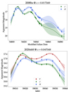 |
Fig. A.1. PISCOLA light-curve fits to SNe 2008hs and 2020mbf. |
Appendix B: NIR light-curve standardization with color components
Figures B.1 and B.2 show the corner plot and Hubble diagram, respectively, using the (Y − H) color-curve PCA coefficients for the standardization (Sect. 6.5). In this case, the standardization is favored by around 3.3σ and 3.7σ significance for p0 and p1, respectively, while σint is significantly reduced from 0.27 mag to 0.16 mag. The reader should have in mind that this sample is smaller than the Y-band only sample given the need of two bands, which explains the difference in σint.
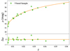 |
Fig. B.2. Y-band Hubble diagram with the standardization from Fig. B.1. The Hubble residual presents a RMS of 0.15 mag and a normalized median absolute deviation of 0.16 mag. |
All Tables
All Figures
|
Fig. 1. PISCOLA light-curve (YJH-bands) fits of three SNe Ia: 2005df (Literature; top), 2008gp (CSP; middle), and 2020jjf (DEHVILS; bottom). The photometric uncertainties propagates into the fits themselves. |
| In the text | |
|
Fig. 2. SNe Ia rest-frame light curves after the preprocessing steps of Sect. 5.1. The phase range covers from −8 to +34 days with respect to optical peak. The light curves are color-coded by sBV value, obtained with SNooPy fits using the max_model model, limiting the color range between 0.8 ≤ sBV ≤ 1.2 for visualization purposes, as the bulk of the sample falls within this range. |
| In the text | |
|
Fig. 3. PCA decomposition for the Y- (top row), J- (middle row), and H-band (bottom row) light curves. Color-coded are the contributions of each of the coefficients with a 2σ range: p0 (left column), p1 (middle column), and p2 (right column). The sample mean is shown as a solid red line. The values in parentheses are the percentages of the explained variance. Three components explain ∼90% of the variance for each of the bands. |
| In the text | |
|
Fig. 4. Comparison of the first (p0; top row) and second (p1; bottom row) PCA coefficients vs. the peak absolute magnitude for each NIR band. The Pearson correlation coefficient (ρ) and p-value for each of the comparisons, with their respective 1σ uncertainty estimated by Monte-Carlo sampling, are shown with the respective linear relations (red lines). The null-hypothesis is that there is no correlation (zero slope). The panels have the same x- and y-axis ranges for visualization purposes. |
| In the text | |
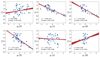 |
Fig. 5. Same as Fig. 4, but for sBV, obtained with SNooPy using the max_model. |
| In the text | |
|
Fig. 6. Comparison between B- (top panels) and V-band (bottom panels) peak absolute magnitudes versus p1 for the Y band (left panels) and p0 for the J band (right panels). |
| In the text | |
|
Fig. 7. Comparison between host-galaxy stellar mass, log10(M/M⊙) and p0. The vertical dashed line marks p0 = 0.0, dividing the SN Ia sample at the mean, while the horizontal lines mark log10(M/M⊙) = 10, commonly used for splitting SNe Ia samples into high- and low-mass hosts. |
| In the text | |
|
Fig. 8. Same as Fig. 2, but for the color-curves: (Y-J) (top panel), (Y-H) (middle panel), and (J-H) (bottom panel). |
| In the text | |
|
Fig. 9. Same as Fig. 3, but for PCA decomposition of the SNe Ia color curves: (Y-J) (top row), (Y-H) (middle row), and (J-H) (bottom row). |
| In the text | |
|
Fig. 10. sBV vs. PCA p0 coefficient for the NIR color curves. |
| In the text | |
|
Fig. 11. B-band (left panels) and V-band (right panels) peak absolute magnitude vs. PCA p0 coefficient for the NIR color curves. |
| In the text | |
|
Fig. 12. Comparison between log10(M/M⊙) (top panels) and E(B−V)host (bottom panels) vs. p0 for the NIR colors. |
| In the text | |
|
Fig. 13. Corner plot of the MCMC posterior distributions used for building a Y-band Hubble diagram. σint is the intrinsic scatter, i.e., leftover scatter unexplained by the standardization. The solid lines show the mean of the distributions while the dashed lines show the 16th and 84th percentiles (1σ). |
| In the text | |
|
Fig. 14. Y-band Hubble diagram with the standardization from Fig. 13. The solid line represents the fitted cosmology, a flat ΛCDM cosmological model with Ωm = 0.3 and H0 = 70 km s−1 Mpc−1. The Hubble residual presents a RMS of 0.27 mag and a normalised median absolute deviation of 0.10 mag. |
| In the text | |
|
Fig. A.1. PISCOLA light-curve fits to SNe 2008hs and 2020mbf. |
| In the text | |
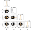 |
Fig. B.1. Same as Fig. 13, but using the PCA decomposition on the (Y − H) color curves. |
| In the text | |
|
Fig. B.2. Y-band Hubble diagram with the standardization from Fig. B.1. The Hubble residual presents a RMS of 0.15 mag and a normalized median absolute deviation of 0.16 mag. |
| In the text | |
Current usage metrics show cumulative count of Article Views (full-text article views including HTML views, PDF and ePub downloads, according to the available data) and Abstracts Views on Vision4Press platform.
Data correspond to usage on the plateform after 2015. The current usage metrics is available 48-96 hours after online publication and is updated daily on week days.
Initial download of the metrics may take a while.