| Issue |
A&A
Volume 702, October 2025
|
|
|---|---|---|
| Article Number | A183 | |
| Number of page(s) | 12 | |
| Section | Extragalactic astronomy | |
| DOI | https://doi.org/10.1051/0004-6361/202555105 | |
| Published online | 20 October 2025 | |
An ALMA Band 7 survey of SDSS/Herschel quasars in Stripe 82
I. The properties of the 870 micron counterparts
1
ESO, Karl-Schwarzschild-Str. 2, 85748
Garching bei München, Germany
2
Instituto de Astrofísica de Canarias, 38205
La Laguna, Tenerife, Spain
3
Departamento de Astrofísica, Universidad de La Laguna, 38206
La Laguna, Tenerife, Spain
4
Joint ALMA Observatory, Alonso de Córdova 3107, Vitacura, 763-0355
Santiago, Chile
5
European Southern Observatory, Alonso de Córdova 3107, Vitacura, Casilla 19001
Santiago, Chile
6
Departamento de Física Teórica e Experimental, Universidade Federal do Rio Grande do Norte, Campus Universitário, Natal RN, 59072-970
Brazil
7
Astronomical Institute, Czech Academy of Sciences, Bocní II 1401, CZ-141 00
Prague, Czech Republic
8
Institute for Astronomy, University of Hawai’i, 2680 Woodlawn Dr., Honolulu, HI, 96822
USA
9
Department of Physics and Astronomy, University of Hawai’i at Mānoa, 2505 Correa Rd., Honolulu, HI, 96822
USA
10
INAF – Osservatorio Astrofisico di Arcetri, Largo E. Fermi 5, I-50125
Firenze, Italy
11
Cosmic Dawn Center (DAWN), Copenhagen, Denmark
12
DTU Space, Technical University of Denmark, Elektrovej 327, 2800
Kgs. Lyngby, Denmark
13
Niels Bohr Institute, University of Copenhagen, Jagtvej 128, 2200
Copenhagen, Denmark
14
Department of Physics and Astronomy, Texas A&M University, College Station, TX, 77843-4242
USA
15
George P. and Cynthia Woods Mitchell Institute for Fundamental Physics and Astronomy, Texas A&M University, College Station, TX, 77843-4242
USA
⋆ Corresponding author: This email address is being protected from spambots. You need JavaScript enabled to view it.
Received:
10
April
2025
Accepted:
30
July
2025
Abstract
Context. Over the past 15 years, studies of quasars in the far-infrared (FIR) have reported host luminosities ranging from 1012 to 1014 L⊙. These luminosities, often derived from Herschel/SPIRE photometry, suggest star formation rates (SFRs) of up to several thousand M⊙ yr−1, positioning them among the most luminous starburst galaxies in the Universe. However, owing to the limited spatial resolution of SPIRE, there is considerable uncertainty regarding whether the FIR emission originates from the quasar itself, nearby sources at the same redshift, or unrelated sources within the SPIRE beam. To resolve this uncertainty, high-resolution observations at wavelengths close to the SPIRE coverage are required to pinpoint the true source of the FIR emission.
Aims. The aim of the present work is to unambiguously identify the submillimetre (submm) counterparts of a statistical sample of FIR bright SDSS quasars and estimate the real multiplicity rates among these systems. We study the evolution of the incidence of multiplicities with redshift, FIR properties, and ‘balnicity’. Based on these multiplicities, we assess the importance of mergers as triggers for concomitant accretion onto supermassive black holes (SMBHs) and extreme star formation.
Methods. We conducted ALMA Band 7 continuum observations of 152 SDSS FIR bright quasars in Stripe 82, covering redshifts between 1 and 4, with a spatial resolution of 0.8″. We identified all sources detected in the Band 7 maps at or above 5σ and performed forced photometry on the phase centre for the few quasars that were not detected otherwise. Additionally, we examined the coarse Band 7 spectra for any serendipitous detections of CO and other transitions.
Results. We find that in approximately 60% of all cases, the submm emission originates from a single counterpart within the SPIRE beam, centred on the optical coordinates of the quasar. The rate of multiplicity increases with redshift, rising by a factor of ∼2.5 between redshifts 1 and 2.5. The incidence of multiplicities is consistent among broad absorption line (BAL) quasars and non-BAL quasars. The multiplicities observed in a fraction of the sample indicate that, while mergers are known to enhance gas inflow efficiency, there must be viable alternatives for driving synchronous SMBH growth and intense star formation in isolated systems. Additionally, we report the serendipitous detection of two CO(6–5) and three CO(7–6) transitions in five quasars at redshifts between 1 and 1.4, out of the eight such transitions expected based on the spectral setup and the redshifts of the objects in the sample. Higher transitions, although expected in a fraction of the sample, are not detected, indicating that the quasars are not sufficiently exciting the gas in their hosts. Finally, we also detect a potential emission of H2O, HCN (10–9), or a combination of both in the spectrum of a quasar at redshift 1.67.
Key words: techniques: interferometric / galaxies: active / quasars: general / galaxies: starburst / radio continuum: galaxies
© The Authors 2025
 Open Access article, published by EDP Sciences, under the terms of the Creative Commons Attribution License (https://creativecommons.org/licenses/by/4.0), which permits unrestricted use, distribution, and reproduction in any medium, provided the original work is properly cited.
This article is published in open access under the Subscribe to Open model. This email address is being protected from spambots. You need JavaScript enabled to view it. to support open access publication.
1. Introduction
Accretion onto supermassive black holes (SMBHs) and starburst activity are known to often occur concomitantly (e.g. Farrah et al. 2003; Lutz et al. 2008; Hernán-Caballero et al. 2009; Hatziminaoglou et al. 2010; Santini et al. 2012; Drouart et al. 2014; Pitchford et al. 2016; Magliocchetti 2022, just to name a few). Both processes draw from common gas reservoirs, possibly fed by major-merger-induced strong inflows (e.g. Di Matteo et al. 2005; Hopkins et al. 2006a,b). While galaxy interactions make gas available for fuelling both SMBH growth and intense star formation, the same gas may become unavailable through the ejection of energy by massive outflows driven by the accretion itself; these two processes seem to be in perpetual competition with one another. Furthermore, the triggering mechanisms of active galactic nuclei (AGN) can change with redshift, with major mergers dominating above a redshift of ∼1.5 and secular mechanisms being more important at lower redshifts (Draper & Ballantyne 2012).
Despite decades of observational and modelling efforts to understand the interplay between intense star formation and accretion onto SMBHs, the precise effects of these processes on each other and on the evolution of massive galaxies remain poorly constrained. This gap in knowledge highlights the importance of studying objects where both phenomena occur simultaneously, as they serve as key laboratories for advancing our understanding of the most fundamental aspects of galaxy evolution.
Such objects are optically and far-infrared (FIR) bright quasars. Indeed, a small fraction (∼5–8%) of optically bright Sloan Digital Sky Survey (SDSS1) quasars, with bolometric luminosities 1045 ≤ Lbol ≤ 1047 erg/s derived by the SDSS pipeline, show extraordinarily high FIR luminosities (in the range 1012 to 1014 L⊙), based on their individual (as opposed to stacked) Herschel fluxes observed with the Spectral and Photometric Imaging Receiver (SPIRE; Griffin et al. 2010) at 250, 350, and 500 μm (Cao Orjales et al. 2012; Pitchford et al. 2016; Kirkpatrick et al. 2020). Such high FIR luminosities suggest star formation rates (SFRs) of up to a few thousand M⊙ yr−1, even after accounting for the contribution of the AGN to the FIR, placing these systems among the most luminous starburst hosts in the Universe. These SFRs are three to ten times higher than the average SFRs of the remaining 95% of SDSS quasars (undetected in the FIR down to the Herschel/SPIRE limits), estimated by stacking Herschel/SPIRE fluxes (Harrison et al. 2012; Mullaney et al. 2015; Harris et al. 2016). SDSS FIR bright quasars, which appear to be undergoing simultaneous episodes of intense star formation and SMBH growth near the Eddington limit, serve as ideal laboratories for studying the physical conditions and environments that trigger and sustain both processes in parallel.
The high SFRs observed in the hosts of bright quasars, which are thought to be quenching or even suppressing star formation (e.g. Page et al. 2012), are surprising. As these SFR estimates are primarily based on FIR flux measurements, often from Herschel/SPIRE, the uncertainty in identifying the correct FIR counterparts also impacts their reliability. Counterpart identification has long been a challenge in FIR surveys (Wang et al. 2014; Hurley et al. 2017), and it remains uncertain whether the SFRs derived for these quasar hosts are even associated with their hosts. Furthermore, given SPIRE’s spatial resolution of 18″ at 250 μm (Griffin et al. 2010), it is likely that in some cases multiple sources contribute to the observed FIR emission. The presence of two or more sources within the SPIRE beam may suggest close pairs, and this proximity could be the trigger for these two extreme phenomena. Accurate identification of the origin of the FIR emission is, therefore, crucial.
Interferometric observations (Hodge et al. 2013; Bussmann et al. 2015; Trakhtenbrot et al. 2017; Stach et al. 2018; Nguyen et al. 2020) have shown that a fraction of single-dish submillimetre (submm) or Herschel sources are blends of multiple galaxies. The fraction of multiple sources varies between 30% and 70% depending on the sensitivity of the submm observations, the nature of the objects, the sample selection, and the definition of multiplicity. Simulations, on the other hand, tend to predict a higher multiplicity fraction than what is observed on average (Hayward et al. 2013; Cowley et al. 2015), possibly due to the assumptions that go into the triggering mechanisms of submillimetre galaxies (SMGs).
In addition to the uncertainties on the source of the FIR emission, the source of heating of the cold dust in the hosts of AGN is also a topic that has not yet been fully resolved. Although star formation is considered to be the driving mechanism (e.g. Hatziminaoglou et al. 2010; Pitchford et al. 2016; Lamperti et al. 2021), some studies indicate that, in at least some cases, the cold gas may be directly heated by the AGN (e.g. Symeonidis 2017; Maddox et al. 2017). More direct evidence may come from the excitation level of the molecular gas in the hosts of the FIR bright AGN. Low-J CO transitions are believed to trace gas within photodissociation regions (PDRs) heated by far-UV radiation, while high-J lines are tracers of X-ray-dominated regions (Wolfire et al. 2022), from the CO(4–3) transition and upwards (Esposito et al. 2024). Nevertheless, Farrah et al. (2022) only found the CO(10–9) transition and above to be increasingly excited by the AGN. Along similar lines, Valentino et al. (2021) suggest that the AGN has only a marginal effect on the CO, at least up to CO(7–6). Earlier studies also indicate that even the higher CO transitions in nearby galaxies can be explained by PDRs (Rigopoulou et al. 2013).
To address the source of FIR emission in SDSS quasars, a pilot study of 28 FIR bright SDSS quasars at redshifts between 2 and 4 was conducted with the Atacama Compact Array (ACA) in Band 7 (Hatziminaoglou et al. 2018). The study, primarily aimed at investigating the issue of multiplicities around quasars, found that about a third of these quasars show clear evidence of secondary counterparts contributing at least 25% to the total 870 μm continuum flux within the SPIRE beam. For a few sources, the FIR emission was not associated with the SDSS quasar at all, but instead originated from a different source. The same study suggested that broad absorption line (BAL) quasars might exhibit higher multiplicity rates (57%) compared to non-BAL quasars (24%), indicating that BAL and non-BAL quasars may reside in different environments. However, these results are limited by low-number statistics (only seven BAL quasars among the 28 objects in the sample). Given the small sample size, the coarse resolution of the ACA (∼4″), and the relatively narrow redshift range, the results, while suggestive, were neither conclusive nor fully representative.
The present paper builds upon the pilot study and presents the results from submm observations of 152 FIR bright SDSS quasars, conducted with the ALMA 12-m Array in Band 7 (870 μm) at a resolution of 0.8″. The primary aim is to verify the findings from the previous study. Specifically, this paper focusses on the multiplicities and serendipitous detections of CO transitions and their implications. A forthcoming paper (Hatziminaoglou et al., in prep.) revisits the spectral energy distribution (SED) fitting and derived SFRs discussed in Pitchford et al. (2016), and further examines the properties of the cold dust in the quasar hosts.
The structure of this paper is as follows. Sections 2 and 3 describe the quasar sample and the ALMA data, respectively. Section 4 discusses the ALMA detections in the quasar fields and the findings related to multiplicities, while Sect. 5 presents serendipitous detections of intermediate CO transitions. The paper concludes with a discussion of the results in the context of recent literature in Sect. 6.
2. ALMA SDSS quasars sample
The quasar sample under study is drawn from the parent sample of FIR bright SDSS quasars in the HerMES (Oliver et al. 2012) fields analysed in Pitchford et al. (2016). It includes a total of 152 FIR bright (S250 ≥ 30 mJy) type 1 SDSS quasars from the SDSS Data Release 7 (Schneider et al. 2007) and Data Release 10 (Pâris et al. 2014) (1045 ≤ Lacc ≤ 1047 erg s−1), in the redshift range 1 ≤z≤ 4, lying in the Herschel Stripe 82 Survey (HerS; Viero et al. 2014). This survey consists of 79 deg2 of contiguous SPIRE imaging of the SDSS Stripe 82 and has excellent quality SPIRE 250, 350, and 500 μm fluxes, extracted following Hurley et al. (2017), as well as a wealth of ancillary multi-wavelength data. These include UV data from the Galaxy Evolution Explorer (GALEX; Morrissey et al. 2007), near-infrared observations from the UKIRT Infrared Deep Sky Survey (UKIDSS; Hewett et al. 2006) and the VISTA Hemisphere Survey (VHS; McMahon et al. 2021), mid-infrared coverage from the Wide-field Infrared Survey Explorer (WISE; Wright et al. 2010), and 1.4 GHz observations from the Faint Images of the Radio Sky at Twenty-cm (FIRST; White et al. 1997). The properties of the sample are shown in Fig. 1.
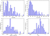 |
Fig. 1. Properties of the sample of 152 quasars. From left to right and top to bottom: spectroscopic redshift; Herschel/SPIRE 250 μm flux (S250); quasar bolometric luminosity (Lbol); and Eddington ratio (λEdd) from the SDSS DR16 catalogue. |
As the parent sample was drawn from more than a decade-old SDSS data releases, the quasars in the sample were checked against the SDSS Data Release 16 (DR16) quasar catalogue, which encompasses all of the quasars from previous releases (for details see Lyke et al. 2020). The quasar nature and the redshifts of all sources remain unchanged in the DR16 catalogue with respect to the previous data releases. The sample is the largest ever observed in the submm with a uniform resolution. To the best of our knowledge, the 152 quasars are not lensed.
Included in this sample are high-ionisation BAL (HiBAL) quasars, which exhibit distinct spectral signatures. These quasars are characterised by strong, broad absorption features in C IV at 1549 Å, indicative of the presence of high-velocity outflows of ionised gas surrounding the quasar. Absorption of Mg II at 2798 Å is associated with low-ionisation BAL quasars (LoBALs) and is typically weaker and narrower than the C IV absorption.
For the SDSS DR16 quasar catalogue, an automatic procedure was implemented to identify HiBAL quasars based on the values of the balnicity and intrinsic absorption indices (BI and AI, respectively), derived mainly from the C IV emission line, as described in (Lyke et al. 2020). Following this procedure, 17 of the quasars in our sample have BAL_PROB = 1.0 (unambiguous BAL identifications) and another 17 have BAL_PROB = 0.9 based on their AI, which are also considered as almost unambiguous BAL quasars. The BI of these quasars is zero where the trough is less than 2000 km s−1 wide and/or the trough extends closer to the line centre than 3000 km s−1. We visually inspected the spectra of these 34 BAL quasars. Of the 17 objects with BAL_PROB = 1.0, 15 show C IV absorption as expected, while two do not present any C IV or Si IV absorption but instead display strong Lyα absorption. Of the 17 objects with BAL_PROB = 0.9, 16 present unambiguous BAL features. The remaining one is excluded from further consideration. Notably, only one object among the 33 shows an absorption in Mg II (SDSS_J014905.28-011404.9), and could therefore be classified as a LoBAL quasar.
3. ALMA data
The ALMA data presented in this work were acquired under Cycle 9 project 2022.1.00029.S (PI Hatziminaoglou) in Band 7. The sample was divided by the ALMA Observing Tool algorithm into three scheduling blocks (SBs), containing 30, 59, and 63 objects, respectively. All targets were observed with the default Band 7 continuum spectral setup, centred at 343.5 GHz sky frequency (rest-frame 0.69–1.7 THz, i.e. 435–176 μm), with the lowest possible spectral resolution (∼28 km/s), in Time Division Mode (TDM).
One SB was observed on October 24, 2022, the other two on October 26, 2022, in configuration C2 with 42–43 usable antennas covering baselines between 14 and 368 m, yielding a 0.8″ spatial resolution. The precipitable water vapour (PWV) ranged from 0.3–0.5 mm, while the phase RMS was 9 − 24 deg measured inter-scan on the phase calibrator. Further water vapour radiometer (WVR; 1 sec scales) solutions were adopted allowing median factor improvements of 1.2–2.6, resulting in overall phase RMS values of 5–11 deg. Thus, the expected signal decorrelation under such conditions is minimal (≲2%), well within the absolute flux uncertainty of 10% in Band 7. As a result, no self-calibration was performed on the sample, particularly because it would only be possible in a small fraction of the sample given their fluxes (see Sect. 4.1). Each science target was observed for 48.2 seconds. Sources J2258-2758 and J0238+1636 were adopted as bandpass calibrators, while J0108+0135 and J0217+0144 were used as phase calibrators. All data were reduced using the ALMA pipeline, version 2022.2.0.64, with Common Astronomy Software Applications (CASA) version 6.4.1.12, with robust 0.5.
4. The properties of the ALMA 870 micron sources
4.1. Identification of submm sources
We automated the source extraction procedure with a custom-made Python script, which includes the identification of secondary counterparts, submm flux measurement, and fitting on the ALMA Band 7 continuum maps. The steps in the script are as follows:
-
Computation of noise levels, including the median absolute deviation (MAD) and the root mean square (RMS) using only pixels within ±5×MAD;
-
Identification of peak fluxes above 5σ;
-
Extraction of the flux density within a box-shaped aperture centred on the peak pixel, with a width twice the beam major axis;
-
For each detected source, determination of the peak flux and S/N, computation of the light-weighted centroid of the intensities above 3σ, and measurement of the distance and position angle from the phase centre;
-
Use of the CASA IMFIT task to fit the emission within a elliptical aperture twice the beam size, maintaining the same major-to-minor axis ratio and position angle, centred on the light-weighted centroid;
-
For quasars with no peak flux above 5σ, photometry extraction at the phase centre was forced as described in point 3, with an attempt to run IMFIT only if the peak flux was above 3σ.
The above procedure resulted in the extraction of 209 Band 7 sources in the 152 quasar fields, described in the next section. For 135 of the 152 quasars (89%), the counterparts were centred on the optical coordinates with peak fluxes above 5σ. For the 17 quasars not detected above 5σ, forced photometry was performed at the location of the quasar, with seven of these yielding detections at or above 3σ. The remaining ten objects with peak fluxes below 3σ are considered as non-detections in the submm and are excluded from further discussion.
Of the 152 quasar fields, 94 (62%) have a single submm counterpart, with two of these located more than 1″ away from the central quasar’s coordinates, and thus not related to the primary source. In 42 fields (28%), two submm counterparts are detected, while nine fields (6%) host three counterparts. One field contains four submm sources. In one of the fields with two counterparts and in one with three, the central quasar was not detected at 870 μm. Secondary counterparts are located between 1″ and ∼10″ from the quasar’s phase centre (Fig. 2, left panel), corresponding to projected physical distances between ∼10 and ∼90 kpc. The right panel of Fig. 2 displays the 870 μm flux distribution for the 209 submm sources (open black histogram). The shaded histogram shows only the primary sources, i.e. the 142 counterparts coinciding within < 0.5″ from the optical coordinates of the quasars. Table 1 presents the first five entries of the submm detections list, with the column descriptions given in the table caption. The full table is available at the CDS. Figure 3 illustrates examples of submm detections in six fields.
First five entries of the ALMA Band 7 photometric catalogue in the fields of the 152 quasars.
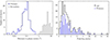 |
Fig. 2. Left: Histogram of the distance to the phase centre for the primary (open histogram) and secondary (grey histogram) counterparts. Right: Distribution of the Band 7 (870 μm) peak fluxes of the 209 ALMA sources in the 152 quasar fields (black histogram). Primary counterparts, that is, those extracted at the phase centre (i.e. at the optical coordinates of the quasars), are shown in a shaded histogram. |
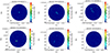 |
Fig. 3. Example ALMA Band 7 images. From top to bottom and left to right: J010524.39-002527.1: single 870 μm counterpart centred on the SDSS coordinates; J021417.64-010524.8: ALMA 870 μm counterpart centred at the location of the quasar, with secondary counterpart; J015017.71+002902.4: ALMA 870 μm counterpart centred at the location of the quasar, with two secondary, brighter counterparts; J005921.54+004350.0: single 870 μm counterpart, not associated with the SDSS quasar; J014555.58-003125.8: three 870 μm counterparts, none of which are associated with the quasar; and J020327.40-001625.9: no detection. The ALMA beam is shown as a black ellipse at the bottom left corner of each image. |
The ten quasars (7% of the sample) with no primary submm counterpart are noteworthy, as they may indicate issues with the FIR data or the association of FIR counterparts to the optical sources. Among these ten cases, one lacks a 500 μm detection and five have 500 μm fluxes below 11.5 mJy (the median of the sample is 22.5 mJy). The remaining four non-detections are in fields with secondary submm sources, suggesting that the FIR emission likely originates from unrelated sources rather than the quasar host.
4.2. Multiplicities as a function of FIR properties, redshift, and balnicity
Scudder et al. (2016) studied the multiplicity of 250 μm Herschel sources in the COSMOS field using Bayesian inference methods. They report that for sources with more than one counterpart and 250 μm fluxes above 45 mJy, the brightest and second brightest components are assigned comparable fluxes, the sum of which does not reach the total 250 μm flux of the SPIRE source. For fainter objects with 250 μm fluxes below 45 mJy, the majority of the 250 μm flux originates from a single bright component. The second brightest component, when present, is typically much fainter.
The above results are not in agreement with our findings. Examining the contribution of the multiple submm counterparts to the total 870 flux on each map, we find that the majority of objects (48 of the 74, or 64.9% ± 9.4%) with S250 < 45 mJy have a single submm counterpart. In the presence of a secondary submm counterpart, the brightest source accounts for approximately 60% of the 870 μm flux within the SPIRE beam, while the secondary source accounts for 42% ± 4% of the total submm flux. The picture is very similar for the bright SPIRE sources with S250 > 45 mJy. We find that 44 of the 78 (56.4% ± 8.5%) have single submm counterparts. Once again, when a secondary counterpart is present, the primary counterpart accounts for approximately 60% of the submm flux, with the secondary contributing 37% ± 10%. Of the 78 sources with S250 > 45 mJy, only eight have a tertiary counterpart; its contribution to the total 870 μm flux does not exceed 20%. In summary, we do not see any significant change in the number of submm counterparts as a function of 250 μm flux. In the presence of multiple counterparts, the primary counterpart typically contributes about 60% to the total submm flux, with the secondary accounting for most of the rest. Some cases require a third counterpart that contributes up to 20% to the total flux. These results are illustrated in Fig. 4, which corresponds to Fig. 4 in Scudder et al. (2016).
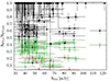 |
Fig. 4. Contribution of the brightest (filled black circles), second brightest (open green circles), and third brightest (open red triangles) counterparts to the total 870 μm flux in each ALMA Band 7 map, shown as a function of the 250 μm originally associated with each SDSS quasar. |
Since multiplicities may indicate over-dense environments around the central quasar, we also examined multiplicities as a function of redshift. Table 2 lists the number of non-detections (discussed above) and quasars with more than one submm counterpart within their respective fields. We note that the incidence of multiplicity increases by a factor of approximately two or more between redshifts 1 to 2.5. Importantly, no dependence of multiplicity is observed with λEdd. The implications of the above findings are discussed in Sect. 6.
Non-detections and multiple components per redshift bin, with Poisson errors.
The sample of 152 quasars includes 33 visually confirmed HiBAL quasars, 17 with BAL_PROB = 1.0 and 16 with BAL_PROB = 0.9 (see Sect. 2). Among the objects with BAL_PROB = 1.0, seven (41% ± 16%) have at least one secondary counterpart, including the two with strong Lyα absorption. Among the 16 objects with BAL_PROB = 0.9, six (38% ± 15%) have at least one secondary counterpart. The only LoBAL quasar in the sample (SDSS_J014905.28-011404.9) does not have a secondary submm counterpart. The incidence of multiplicities among the BAL quasars does not differ from that observed in the full sample, demonstrating that previous claims of dependency with balnicity were driven by low-number statistics.
5. Serendipitous line detections
Given the broad redshift range, the size and nature of the sample, and despite the very coarse spectral resolution, some of the main CO transitions are expected to be present in the spectra of some targets, redshifted into the survey spectral coverage. In particular, the CO transitions from CO(6–5) to CO(15–14) fall within the frequency range covered by our sample. For the redshifts of the objects in the sample, with a redshift uncertainty of 0.002 (typical for SDSS quasars, as derived from principal component analysis methods; Lyke et al. 2020), and considering the Band 7 continuum spectral setup (which consists of four spectral windows, each 1.875 GHz wide and centred at 336.5, 338.5, 348.5, and 350.5 GHz), a total of 31 CO transitions fall within the spectral range covered by the ALMA observations. These include three CO(6–5), five CO(7–6), eight CO(8–7), five CO(9–8), and ten CO(10–9) and higher-J transitions.
ALMA spectra were extracted for all 209 detections and visually inspected. The extraction was performed within an aperture with the size and position angle of the synthesised beam. A detection was considered reliable if the peak of the binned spectrum exceeded the 3σ per-channel level and was supported by the existence of a nearby transition within a velocity shift compatible with the error on the redshift (see also the caption of Fig. 5). A visual inspection was also performed on all the plots produced by the ALMA pipeline runs at the step of continuum finding, available in the pipeline logs.
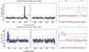 |
Fig. 5. Band 7 spectra of the two quasars with unambiguous CO(6–5) transition detections. Left and middle columns: Filled blue histograms show extracted spectra within the extraction aperture, smoothed to a spectral resolution of ∼111 km s−1, while the solid black histogram shows the raw-resolution spectra of the peak flux within the aperture (units of Jy/beam). The shaded grey regions represent per-channel ±1σ, while the dotted lines indicate the per-channel ±3σ level. The magenta line shows the continuum subtracted from the spectrum to assess the significance of absorption detections (none detected). Dashed red lines indicate the expected location of the CO transition shifted to the optical (SDSS) redshift of each object. The orange line shows the single-Gaussian fit to the line. Right column: ALMA pipeline continuum fitting output from the spectral window where the lines were identified. The binned spectrum in red; the region in which the continuum has been extracted is shown in cyan; and the level of the continuum is shown in black. The x axis at the bottom indicates the channels, and the x axis at the top indicates the frequency (in GHz). These plots were extracted directly from the logs of the pipeline runs (‘weblogs’). |
No transitions higher than CO(7–6) were identified in the low-resolution ALMA spectra. Two of the three expected CO(6–5) lines (rest frequency of 691.473 GHz) are clearly visible in the spectra of the objects (SDSS_J010249.02–010544.8 and SDSS_J011922.85–004419.7). The third source (SDSS_J013109.99+010612.8) shows no sign of emission in its spectrum and is, in fact, undetected at 870 μm, with no other submm sources detected in its vicinity. The quasar has an estimated SFR (derived by Pitchford et al. 2016) of ∼520 M and is accreting at a λedd of 0.03, both at the very low end of the parameter distribution in the sample. Figure 5 shows the extracted spectra split by baseband in the left and middle panels. The right panel shows the ALMA pipeline continuum fitting output from the spectral window in which the identified transition is located.
Of the five expected CO(7–6) transitions (rest frequency 806.651 GHz), three are detected in the spectra: SDSS_J013523.49+001046.3, SDSS_J013150.85–002701.8, and SDSS_J011032.18-010320.4. These are shown in Fig. 6. The remaining two, which were not detected, were associated with quasars both detected above 5σ on the Band 7 maps, one of which has a secondary counterpart at a distance of 6.6″.
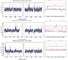 |
Fig. 6. Same as Fig. 5, but for CO(7–6) transitions. The expected location of the nearby CI(2–1) transition is also marked on the plots; however, these transitions are not detected at a significant level. |
The five detected CO transitions are all shifted with respect to the frequency corresponding to the optical (SDSS) redshift by between 0.1 and 0.5 GHz, equivalent to velocity shifts between 85 and 440 km s−1. These shifts equate to redshift differences of 0.002 or less, within the uncertainties of the SDSS redshift values. The transitions, observed frequencies, significance of the detections, and integrated fluxes are shown in Table 3.
Of the three objects with expected CO(6–5) lines and the five with expected CO(7–6) lines, only one has a secondary counterpart, at a distance of 6.6″ from the phase centre. No lines are present in the spectrum of this source and no secondary counterparts show convincing line emission in the automated search.
In addition, we identified a possible detection of H2O at a rest frequency of 906.205 GHz, HCN(10–9) at a rest frequency of 906.24 GHz, or a combination of the two. This tentative detection is shown in Fig. 7.
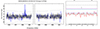 |
Fig. 7. Detection of H2O 92, 8 − 83, 5, HNC (10-9), or a combination of both in the spectrum of SDSS_J020310.10+011327.8. This line was not picked up by the continuum finder of the ALMA pipeline, nor is it visible in the weblog graph (right panel). No Gaussian fit is presented for this line. |
We also carried out an independent, blind search using the Source Finding Application (SoFiA2; Serra et al. 2015). This application provides a selection of emission line searches in data cubes, as well as routines to smooth the cubes spatially and spectrally. Prior to running SoFiA, we removed continuum emission from the cubes either by directly subtracting the continuum image or by removing the median value estimated along the frequency axis. We adopted Gaussian kernels to smooth the cubes spatially (widths of 3, 6, and 9 pixels, for a pixel scale of ∼0.14″) and in velocity (3, 6, 9, 12, 15, and 18-channel smoothing, for ∼28 km/s channel width). For consistency, we ran the same kernels on the inverted cubes for reliability assessment. No additional lines were found by this procedure.
6. Discussion
The purpose of this study was to derive the multiplicity rates around quasars with intense star formation in their hosts, as indicated by their high FIR luminosities. This work complements previous studies that were based on smaller samples and/or lower spatial resolution, aiming to confirm or refute the extremely high SFRs in the hosts of these quasars and to assess the role of the environment on the concomitant accretion onto SMBHs and extreme star formation.
Of the 152 SDSS quasars followed up with ALMA in Band 7 within the framework of this project, 142 are detected at 870 μm at or above 3σ, with 135 detected above 5σ. This sample of submm quasars is the largest observed with a uniform spatial resolution (0.8″). It increases the total number of SDSS quasars observed with ALMA as science targets (see Wong et al. 2023) by approximately 40%, and more than doubles the number of SDSS quasars with ALMA Band 7 detections.
Our analysis shows that approximately one third of the FIR bright quasars have secondary submm counterparts within projected distances of a few to several tens of kpc. At the limited SDSS resolution, none of the quasars in the sample show signs of recent merger activity (i.e. they are point-like and lack features such as tidal tails), but the spatial resolution and sensitivity of SDSS are insufficient for a proper assessment. Furthermore, in the absence of spectroscopic information for the secondary counterparts, it is not possible to determine whether these are physical associations at the redshift of the quasar or chance associations.
The FIR selection of the sample inherently biases it towards systems with more gas and dust, which are also more likely to be involved in mergers. In contrast, SDSS quasars selected optically may exhibit a lower observed merger rate. This may be because they include quasars triggered by secular processes rather than mergers, or because they involve quasars in the late stages of a merger, when multiple counterparts are more difficult to resolve.
6.1. Multiplicities and associations
To assess the probability that the secondary submm counterparts identified in the present analysis are not chance associations, but rather physical pairs or triplets, we compared the number counts in the quasar fields with those derived from submm number counts at 1.1 mm in deep ALMA fields, namely SSA22 (Umehata et al. 2017) and GOODS-ALMA (Franco et al. 2018). To directly compare 1.1 mm number counts with our 870 μm counts, we scaled the flux density of the counts as S1.1mm/S870 μm = 0.56, following Hatsukade et al. (2016) and Franco et al. (2018). This value was derived assuming a modified blackbody model with a dust emissivity of β = 1.5 (e.g Gordon et al. 2010) and a dust temperature of T = 35 K, typical for SMGs (Kovács et al. 2006). Specifically, we compared the incidence of detected companions with the expected field counts predicted by Umehata et al. (2017, black line/region) and Franco et al. (2018, red line/region). Overall, for the total survey area (152 fields comprising ∼9.8 arcmin2), Umehata et al. (2017) and Franco et al. (2018) predict 6.9 ± 3.9 and 6.3 ± 1.9 serendipitous (i.e. unrelated to the quasars) sources, respectively. This is a factor of ten lower than the total of 67 secondary counterparts detected at 870 μm. The excess is particularly striking up to the distance of 6″, beyond which the counts around the quasars in our sample are consistent, within the errors, with the counts from the deep fields. The comparison is shown in Fig. 8 and is strongly indicative of physical rather than chance associations between the primary and secondary sources.
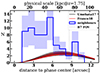 |
Fig. 8. Comparison between the number of sources detected around the quasar sample at separations > 1″ and S/N > 5 (blue, with Poisson errors indicated as shaded regions) and the expected field source counts from Umehata et al. (2017, black) and Franco et al. (2018, red). Red and grey shaded areas indicate the 1σ confidence regions from 1000 bootstrap realisations, based on parameter uncertainties reported in those works. Counts represent the expected number of unrelated serendipitous sources over a total area corresponding to apertures of increasing radius (x axis), accounting for primary beam attenuation; this explains the drop beyond the 0.5 dilution fraction (dotted line). The top axis shows the projected physical scales at the sample’s median redshift (z = 1.75). |
Caution is warranted when interpreting the multiplicities, as results based on Illustris simulations show that projected spatial separation and relative velocity of members of interactive systems are equally important factors in determining the probability that interactive objects will merge (Ventou et al. 2019). Since neither the redshifts of the secondary sources nor their relative velocities are known for the multiple objects in our sample, we cannot assess the probability of these systems being genuine mergers. Nevertheless, at least a fraction of the secondary counterparts must be SMGs, undergoing intense star formation, located at distances suggestive of interacting pairs.
Quasar-quasar or quasar-SMG pairs at high redshift can serve as tracers of the large–scale distribution of galaxies and as proxies for overdense regions (Herwig et al. 2025, but see also Chen et al. 2023, as care must be taken when interpreting overdensities), especially given their high luminosity and dedicated surveys. Multiple studies (e.g. Wylezalek et al. 2013; Silva et al. 2015; Banerji et al. 2021; Izumi et al. 2024) have shown that z > 1.5 quasars are often found in overdense environments rich in dusty, star-forming galaxies, suggesting that mergers are one of the mechanisms for synchronising rapid SMBH growth and star formation in quasar hosts.
Galaxy mergers, particularly major mergers, are known to be linked to quasar activity; however, the precise relationship and its evolution over cosmic time remain complex and actively debated. Some studies report a higher incidence of mergers in quasar host galaxies compared to inactive galaxies, particularly for powerful radio-loud quasars (e.g. Breiding et al. 2024), whereas others find no significant correlation (Marian et al. 2019), leaving results inconclusive, especially at higher redshifts.
Given this context, we interpret the findings of our study as placing an upper limit of ∼30% to the fraction of FIR and optically bright quasars in which a merger event could trigger concomitant accretion onto the central SMBH and intense star formation in their hosts, as well as in the host of the merger partner.
The increase in the multiplicity rate with redshift by a factor of ∼2.5 between redshifts 1 and 2.5, as reported in Sect. 4.2, is consistent with observations of X-ray selected, unobscured AGN in the COSMOS field, which show an increase in the number of AGN with disturbed morphologies (indicative of mergers) by a factor of ∼4 from redshift 0.5 to 2 (Hewlett et al. 2017). Nevertheless, the same study reports a total 15% of AGN with morphologically disturbed hosts, a fraction considerably smaller than the 35% of objects with multiple counterparts reported here that may be part of a merging system. In fact, the fraction of AGN that are part of merging systems at redshifts typically between 1 and 3 varies wildly in the literature, even among the brightest systems, ranging from as low as 10% (Treister et al. 2012) to more than 70% (Glikman et al. 2015).
Approximately 60% of FIR bright SDSS quasars have a single submm counterpart located within 0.5″ of the optical coordinates (see Fig. 2), consistent with the findings of the pilot project (Hatziminaoglou et al. 2018), despite the coarser (by a factor of ∼5) spatial resolution of the data in the pilot study. Excluding projection effects (i.e. companions lying along the line of sight and, hence, undetectable) and post-coalescence phases where mergers would no longer be detectable, and given the absence of disturbed morphologies or tidal features (within the limitations of the available data), these results suggest that, while mergers enhance gas inflow efficiency, there must be other viable alternatives for driving synchronous SMBH growth and extreme star formation. Recent cosmological simulations support the notion that there is little to no connection between mergers and accretion (e.g. Steinborn et al. 2018; Ricarte et al. 2019, and references therein). In these simulations, SMBHs and their hosts assemble in parallel, regardless of their larger-scale environment. Alternative mechanisms to mergers, beyond the commonly invoked bar-type instabilities, include gas inflows via smooth accretion from cosmic filaments or halo reservoirs (Elbaz et al. 2009). Such processes can fuel both star formation and AGN activity without gravitational interactions, particularly in high-redshift environments where cold gas streams are prevalent (Zhu et al. 2024).
Mergers have also been proposed to explain the BAL features observed in ∼20% of optically selected quasars, as the outflows presumably responsible for these features may occur during an early stage in a quasar’s lifetime, when it has been recently (re)fuelled by a merger that also triggers star formation in their hosts. In particular, LoBAL quasars may represent a short-lived transition between a merger-induced starburst and an optically luminous quasar (e.g. Boroson & Meyers 1992). Alternatively, in an orientation-based scenario, BAL winds are present in all quasars in line with the AGN unified model (Antonucci 1993) but can only be viewed along particular lines of sight due to the covering factor of the BAL region (e.g. Becker et al. 2000). The lack of correlation between multiplicity incidence and balnicity reported here, consistent with studies of large samples showing that BAL quasars inhabit environments similar to those of non-BAL quasars (Shen et al. 2008), implies that the BAL phenomenon is likely not driven by, or associated with, differences in the larger-scale dusty or star-forming environments of quasars. Instead, it is likely driven by processes intrinsic to the quasars themselves or their immediate surroundings, supporting the view that BAL and non-BAL quasars belong to the same parent population and differ primarily in orientation or other internal properties, consistent with the line-of-sight scenario. It is worth noting that although the young-phase scenario described above is primarily relevant to the LoBAL quasars, the only object in our sample with characteristics compatible with a LoBAL nature does not have a secondary counterpart.
6.2. Carbon monoxide transitions in the low resolution spectra
Carbon monoxide (CO) is the second most abundant molecule in the Universe and the best tracer of H2 (Solomon & Vanden Bout 2005). Intermediate transitions such as CO(6–5) and CO(7–6) are indicative of the presence of warm and dense molecular gas in the host galaxy’s star-forming regions. Although intermediate CO transitions are seen both at low redshift (e.g. Molyneux et al. 2024, and references therein) and at redshifts above ∼6 (e.g. Bertoldi et al. 2003; Decarli et al. 2022), studies reporting such transitions in quasars at redshifts comparable to those of our sample remain limited. Stacey et al. (2022) and Scholtz et al. (2023) discuss the detection of CO(7–6) in the spectra of strongly reddened quasars, while Balashev et al. (2025) report the detection of CO(7–6) in a quasar – SMG merging system at a redshift of 2.66. To our knowledge, however, no previous studies have reported CO(6–5) emission in quasars at or near cosmic noon, making the two detections presented here the first of their kind.
Within our sample, we detect two of three expected CO(6–5) lines and three of five expected CO(7–6) lines. Assuming a typical CO spectral line energy distribution (COSLED) for quasars, as reported by, e.g. van der Werf et al. (2010) and Carilli & Walter (2013), we estimate that the sensitivity of our ALMA observations is sufficient to detect all CO transitions with Jupp between 6 and 10 at a significance level above 6σ, with the exception of one source that lacks a submm continuum detection. The absence of these higher-J CO lines in the remaining sources therefore indicates that the molecular gas is insufficiently excited to populate these transitions. As such high-J lines require elevated gas temperatures and densities, their non-detection implies moderate excitation conditions without the presence of strong heating or extreme environments. Indeed, CO excitation models (e.g. Meijerink et al. 2007; Kamenetzky et al. 2016) associate high-J line emission primarily with AGN-driven processes. Our conclusions are also consistent with Farrah et al. (2022), who report significant AGN contributions to CO transitions with Jupp = 9 and above only.
For transitions with Jupp ≥ 11, our sensitivity limits detections to at or below the 5σ level, and we therefore refrain from drawing firm conclusions for these higher transitions. Our detection of intermediate-J transitions, combined with the lack of higher-J lines, agrees with the findings of Kirkpatrick et al. (2019), who also observed a lack of high-J CO lines in a similar redshift AGN sample. Both results suggest that the molecular gas resides primarily in a cooler, less dense phase, typical of star-forming galaxies (e.g. Shangguan et al. 2020). Overall, the gas is neither warm nor dense enough to reach the extreme conditions needed for significant high-J CO emission.
To further explore whether the mid-J CO transitions might originate from X-ray-dominated regions (XDRs) as suggested by e.g. Esposito et al. (2024), and thus correlate with the presence of X-ray emission, we searched for X-ray counterparts to our sample in the XMM and Chandra catalogues. We identified 27 matches in the 4XMM-DR14 catalogue (Webb et al. 2020) within 5″ of the SDSS quasar coordinates. Based on their redshifts and the ALMA setup, seven of these sources were expected to exhibit detectable CO lines: one CO(7–6), three CO(8–7), one CO(9–8), one CO(11–10), and one CO(12–11). Of these, only the CO(7–6) transition was detected. The absence of higher-J line detections suggests that XDRs do not significantly impact the molecular gas in these quasar hosts. We also identified eight matches in the Chandra Source Catalogue Release 2.1 (Evans et al. 2024), but none were expected to show CO emission.
Direct comparisons of intermediate-J CO detection rates across redshift remain challenging due to small sample sizes. Decarli et al. (2022) detect CO(7–6) in all ten quasars and CO(6–5) in six of the ten quasars at z ∼ 6, broadly consistent with our findings. In contrast, Salvestrini et al. (2025) report no significant detections in five quasars at z > 7, indicating that quasar hosts during the Epoch of Reionisation likely contained less cold molecular gas than those at lower redshifts. The small number of detections in our work and previous studies prevents firm conclusions. Nonetheless, the combined findings suggest that gas excitation may vary with redshift or quasar luminosity.
Far-infrared H2O transitions are commonly present with intensities comparable to CO transitions, both in the local Universe (e.g. van der Werf et al. 2010) and in high-redshift quasar hosts (van der Werf et al. 2011) and ultra-luminous infrared galaxies (Omont et al. 2013). Using Herschel/SPIRE data, Yang et al. (2013) demonstrated a correlation between the luminosity of submm H2O transitions and infrared luminosity over three orders of magnitude, suggesting that these transitions trace star formation. Our tentative detection of H2O in the host of a FIR bright quasar provides further support for this interpretation.
6.3. Implications of extreme star formation rates
More than half of the z > 1 quasars in the parent sample of Pitchford et al. (2016), as well as 56% of the quasars in our sample, exhibit FIR-derived SFRs exceeding 1000 M⊙ yr−1. The increase in LIR and SFRs with multiplicity strongly suggests that Herschel-derived FIR properties must be carefully evaluated, as at least a fraction of the extreme FIR-based SFRs may result from the contribution of multiple sources to the FIR fluxes.
We address this issue in a forthcoming paper (Hatziminaoglou et al., in preparation) in which the SEDs of the 152 quasars will be re-analysed. In this up-coming work, the 870 μm data point will be incorporated into the optical-to-FIR SEDs of the objects. For sources with multiple submm counterparts within 10″ of the quasar’s optical position, FIR fluxes will be weighted according to their relative 870 μm fluxes. The SED-fitting procedure described in Pitchford et al. (2016) will then be applied derive LIR and SFRs, enabling a direct comparison with our previous findings. This approach will allow for a reassessment of the extreme SFRs in quasar hosts, as well as an analysis of dust temperatures in quasars at redshifts between 1 and 4.
Data availability
The full Table 1 is available at the CDS via https://cdsarc.cds.unistra.fr/viz-bin/cat/J/A+A/702/A183
Acknowledgments
EH acknowledges support from the Fundación Occident and the Instituto de Astrofísica de Canarias under the Visiting Researcher Programme 2022-2024 agreed between both institutions. RS thanks the Coordenação de Aperfeiçoamento de Pessoal de Nível Superior (CAPES–Brasil) and the CAPES-Print program for funding their stay at ESO, as well as ESO for their hospitality in the period April to December 2023 during which part of the work was carried out. A.F. acknowledges support from project “VLT- MOONS” CRAM 1.05.03.07, INAF Large Grant 2022 “The metal circle: a new sharp view of the baryon cycle up to Cosmic Dawn with the latest generation IFU facilities” and INAF Large Grant 2022 “Dual and binary SMBH in the multi-messenger era”. AB acknowledges the support of the EU-ARC.CZ Large Research Infrastructure grant project LM2023059 of the Ministry of Education, Youth and Sports of the Czech Republic. This paper makes use of the following ALMA data: ADS/JAO.ALMA#2022.1.00029.S. ALMA is a partnership of ESO (representing its member states), NSF (USA) and NINS (Japan), together with NRC (Canada), NSTC and ASIAA (Taiwan), and KASI (Republic of Korea), in cooperation with the Republic of Chile. The Joint ALMA Observatory is operated by ESO, AUI/NRAO and NAOJ. This work makes use of TOPCAT (Taylor 2005). Funding for the Sloan Digital Sky Survey IV has been provided by the Alfred P. Sloan Foundation, the U.S. Department of Energy Office of Science, and the Participating Institutions. SDSS-IV acknowledges support and resources from the Center for High Performance Computing at the University of Utah. The SDSS website is www.sdss4.org. SDSS-IV is managed by the Astrophysical Research Consortium for the Participating Institutions of the SDSS Collaboration including the Brazilian Participation Group, the Carnegie Institution for Science, Carnegie Mellon University, Center for Astrophysics | Harvard & Smithsonian, the Chilean Participation Group, the French Participation Group, Instituto de Astrofísica de Canarias, The Johns Hopkins University, Kavli Institute for the Physics and Mathematics of the Universe (IPMU)/University of Tokyo, the Korean Participation Group, Lawrence Berkeley National Laboratory, Leibniz Institut für Astrophysik Potsdam (AIP), Max-Planck-Institut für Astronomie (MPIA Heidelberg), Max-Planck-Institut für Astrophysik (MPA Garching), Max-Planck-Institut für Extraterrestrische Physik (MPE), National Astronomical Observatories of China, New Mexico State University, New York University, University of Notre Dame, Observatário Nacional/MCTI, The Ohio State University, Pennsylvania State University, Shanghai Astronomical Observatory, United Kingdom Participation Group, Universidad Nacional Autónoma de México, University of Arizona, University of Colorado Boulder, University of Oxford, University of Portsmouth, University of Utah, University of Virginia, University of Washington, University of Wisconsin, Vanderbilt University, and Yale University.
References
- Antonucci, R. 1993, ARA&A, 31, 473 [Google Scholar]
- Balashev, S., Noterdaeme, P., Gupta, N., et al. 2025, Nature, 641, 1137 [Google Scholar]
- Banerji, M., Jones, G. C., Carniani, S., DeGraf, C., & Wagg, J. 2021, MNRAS, 503, 5583 [Google Scholar]
- Becker, R. H., White, R. L., Gregg, M. D., et al. 2000, ApJ, 538, 72 [NASA ADS] [CrossRef] [Google Scholar]
- Bertoldi, F., Cox, P., Neri, R., et al. 2003, A&A, 409, L47 [NASA ADS] [CrossRef] [EDP Sciences] [Google Scholar]
- Boroson, T. A., & Meyers, K. A. 1992, ApJ, 397, 442 [NASA ADS] [CrossRef] [Google Scholar]
- Breiding, P., Chiaberge, M., Lambrides, E., et al. 2024, ApJ, 963, 91 [NASA ADS] [CrossRef] [Google Scholar]
- Bussmann, R. S., Riechers, D., Fialkov, A., et al. 2015, ApJ, 812, 43 [Google Scholar]
- Cao Orjales, J. M., Stevens, J. A., Jarvis, M. J., et al. 2012, MNRAS, 427, 1209 [Google Scholar]
- Carilli, C. L., & Walter, F. 2013, ARA&A, 51, 105 [NASA ADS] [CrossRef] [Google Scholar]
- Chen, J., Ivison, R. J., Zwaan, M. A., et al. 2023, A&A, 675, L10 [NASA ADS] [CrossRef] [EDP Sciences] [Google Scholar]
- Cowley, W. I., Lacey, C. G., Baugh, C. M., & Cole, S. 2015, MNRAS, 446, 1784 [Google Scholar]
- Decarli, R., Pensabene, A., Venemans, B., et al. 2022, A&A, 662, A60 [NASA ADS] [CrossRef] [EDP Sciences] [Google Scholar]
- Di Matteo, T., Springel, V., & Hernquist, L. 2005, Nature, 433, 604 [NASA ADS] [CrossRef] [Google Scholar]
- Draper, A. R., & Ballantyne, D. R. 2012, ApJ, 751, 72 [NASA ADS] [CrossRef] [Google Scholar]
- Drouart, G., De Breuck, C., Vernet, J., et al. 2014, A&A, 566, A53 [NASA ADS] [CrossRef] [EDP Sciences] [Google Scholar]
- Elbaz, D., Jahnke, K., Pantin, E., Le Borgne, D., & Letawe, G. 2009, A&A, 507, 1359 [NASA ADS] [CrossRef] [EDP Sciences] [Google Scholar]
- Esposito, F., Vallini, L., Pozzi, F., et al. 2024, MNRAS, 527, 8727 [Google Scholar]
- Evans, I. N., Evans, J. D., Martínez-Galarza, J. R., et al. 2024, ApJS, 274, 22 [NASA ADS] [CrossRef] [Google Scholar]
- Farrah, D., Afonso, J., Efstathiou, A., et al. 2003, MNRAS, 343, 585 [Google Scholar]
- Farrah, D., Efstathiou, A., Afonso, J., et al. 2022, Universe, 9, 3 [Google Scholar]
- Franco, M., Elbaz, D., Béthermin, M., et al. 2018, A&A, 620, A152 [NASA ADS] [CrossRef] [EDP Sciences] [Google Scholar]
- Glikman, E., Simmons, B., Mailly, M., et al. 2015, ApJ, 806, 218 [Google Scholar]
- Gordon, K. D., Galliano, F., Hony, S., et al. 2010, A&A, 518, L89 [NASA ADS] [CrossRef] [EDP Sciences] [Google Scholar]
- Griffin, M. J., Abergel, A., Abreu, A., et al. 2010, A&A, 518, L3 [EDP Sciences] [Google Scholar]
- Harris, K., Farrah, D., Schulz, B., et al. 2016, MNRAS, 457, 4179 [NASA ADS] [CrossRef] [Google Scholar]
- Harrison, C. M., Alexander, D. M., Mullaney, J. R., et al. 2012, ApJ, 760, L15 [NASA ADS] [CrossRef] [Google Scholar]
- Hatsukade, B., Kohno, K., Umehata, H., et al. 2016, PASJ, 68, 36 [NASA ADS] [CrossRef] [Google Scholar]
- Hatziminaoglou, E., Omont, A., Stevens, J. A., et al. 2010, A&A, 518, L33 [NASA ADS] [CrossRef] [EDP Sciences] [Google Scholar]
- Hatziminaoglou, E., Farrah, D., Humphreys, E., et al. 2018, MNRAS, 480, 4974 [Google Scholar]
- Hayward, C. C., Behroozi, P. S., Somerville, R. S., et al. 2013, MNRAS, 434, 2572 [NASA ADS] [CrossRef] [Google Scholar]
- Hernán-Caballero, A., Pérez-Fournon, I., Hatziminaoglou, E., et al. 2009, MNRAS, 395, 1695 [CrossRef] [Google Scholar]
- Herwig, E., Arrigoni Battaia, F., Chen, C. C., et al. 2025, A&A, https://doi.org/10.1051/0004-6361/202555885 [Google Scholar]
- Hewett, P. C., Warren, S. J., Leggett, S. K., & Hodgkin, S. T. 2006, MNRAS, 367, 454 [Google Scholar]
- Hewlett, T., Villforth, C., Wild, V., et al. 2017, MNRAS, 470, 755 [NASA ADS] [CrossRef] [Google Scholar]
- Hodge, J. A., Karim, A., Smail, I., et al. 2013, ApJ, 768, 91 [Google Scholar]
- Hopkins, P. F., Hernquist, L., Cox, T. J., et al. 2006a, ApJS, 163, 1 [Google Scholar]
- Hopkins, P. F., Somerville, R. S., Hernquist, L., et al. 2006b, ApJ, 652, 864 [NASA ADS] [CrossRef] [Google Scholar]
- Hurley, P. D., Oliver, S., Betancourt, M., et al. 2017, MNRAS, 464, 885 [Google Scholar]
- Izumi, T., Matsuoka, Y., Onoue, M., et al. 2024, ApJ, 972, 116 [NASA ADS] [CrossRef] [Google Scholar]
- Kamenetzky, J., Rangwala, N., Glenn, J., Maloney, P. R., & Conley, A. 2016, ApJ, 829, 93 [Google Scholar]
- Kirkpatrick, A., Sharon, C., Keller, E., & Pope, A. 2019, ApJ, 879, 41 [NASA ADS] [CrossRef] [Google Scholar]
- Kirkpatrick, A., Urry, C. M., Brewster, J., et al. 2020, ApJ, 900, 5 [NASA ADS] [CrossRef] [Google Scholar]
- Kovács, A., Chapman, S. C., Dowell, C. D., et al. 2006, ApJ, 650, 592 [CrossRef] [Google Scholar]
- Lamperti, I., Harrison, C. M., Mainieri, V., et al. 2021, A&A, 654, A90 [NASA ADS] [CrossRef] [EDP Sciences] [Google Scholar]
- Lutz, D., Sturm, E., Tacconi, L. J., et al. 2008, ApJ, 684, 853 [NASA ADS] [CrossRef] [Google Scholar]
- Lyke, B. W., Higley, A. N., McLane, J. N., et al. 2020, ApJS, 250, 8 [NASA ADS] [CrossRef] [Google Scholar]
- Maddox, N., Jarvis, M. J., Banerji, M., et al. 2017, MNRAS, 470, 2314 [Google Scholar]
- Magliocchetti, M. 2022, A&ARv, 30, 6 [NASA ADS] [CrossRef] [Google Scholar]
- Marian, V., Jahnke, K., Mechtley, M., et al. 2019, ApJ, 882, 141 [CrossRef] [Google Scholar]
- McMahon, R. G., Banerji, M., Gonzalez, E., et al. 2021, VizieR Online Data Catalog: II/367 [Google Scholar]
- Meijerink, R., Spaans, M., & Israel, F. P. 2007, A&A, 461, 793 [NASA ADS] [CrossRef] [EDP Sciences] [Google Scholar]
- Molyneux, S. J., Calistro Rivera, G., De Breuck, C., et al. 2024, MNRAS, 527, 4420 [Google Scholar]
- Morrissey, P., Conrow, T., Barlow, T. A., et al. 2007, ApJS, 173, 682 [Google Scholar]
- Mullaney, J. R., Alexander, D. M., Aird, J., et al. 2015, MNRAS, 453, L83 [Google Scholar]
- Nguyen, N. H., Lira, P., Trakhtenbrot, B., et al. 2020, ApJ, 895, 74 [NASA ADS] [CrossRef] [Google Scholar]
- Oliver, S. J., Bock, J., Altieri, B., et al. 2012, MNRAS, 424, 1614 [NASA ADS] [CrossRef] [Google Scholar]
- Omont, A., Yang, C., Cox, P., et al. 2013, A&A, 551, A115 [NASA ADS] [CrossRef] [EDP Sciences] [Google Scholar]
- Page, M. J., Symeonidis, M., Vieira, J. D., et al. 2012, Nature, 485, 213 [NASA ADS] [CrossRef] [Google Scholar]
- Pâris, I., Petitjean, P., Aubourg, É., et al. 2014, A&A, 563, A54 [NASA ADS] [CrossRef] [EDP Sciences] [Google Scholar]
- Pitchford, L. K., Hatziminaoglou, E., Feltre, A., et al. 2016, MNRAS, 462, 4067 [NASA ADS] [CrossRef] [Google Scholar]
- Ricarte, A., Tremmel, M., Natarajan, P., & Quinn, T. 2019, MNRAS, 489, 802 [NASA ADS] [CrossRef] [Google Scholar]
- Rigopoulou, D., Hurley, P. D., Swinyard, B. M., et al. 2013, MNRAS, 434, 2051 [Google Scholar]
- Salvestrini, F., Feruglio, C., Tripodi, R., et al. 2025, A&A, 695, A23 [NASA ADS] [CrossRef] [EDP Sciences] [Google Scholar]
- Santini, P., Rosario, D. J., Shao, L., et al. 2012, A&A, 540, A109 [NASA ADS] [CrossRef] [EDP Sciences] [Google Scholar]
- Schneider, D. P., Hall, P. B., Richards, G. T., et al. 2007, AJ, 134, 102 [NASA ADS] [CrossRef] [Google Scholar]
- Scholtz, J., Maiolino, R., Jones, G. C., & Carniani, S. 2023, MNRAS, 519, 5246 [NASA ADS] [CrossRef] [Google Scholar]
- Scudder, J. M., Oliver, S., Hurley, P. D., et al. 2016, MNRAS, 460, 1119 [NASA ADS] [CrossRef] [Google Scholar]
- Serra, P., Westmeier, T., Giese, N., et al. 2015, MNRAS, 448, 1922 [Google Scholar]
- Shangguan, J., Ho, L. C., Bauer, F. E., Wang, R., & Treister, E. 2020, ApJ, 899, 112 [NASA ADS] [CrossRef] [Google Scholar]
- Shen, Y., Strauss, M. A., Hall, P. B., et al. 2008, ApJ, 677, 858 [Google Scholar]
- Silva, A., Sajina, A., Lonsdale, C., & Lacy, M. 2015, ApJ, 806, L25 [NASA ADS] [CrossRef] [Google Scholar]
- Solomon, P. M., & Vanden Bout, P. A. 2005, ARA&A, 43, 677 [NASA ADS] [CrossRef] [Google Scholar]
- Stacey, H. R., Costa, T., McKean, J. P., et al. 2022, MNRAS, 517, 3377 [NASA ADS] [CrossRef] [Google Scholar]
- Stach, S. M., Smail, I., Swinbank, A. M., et al. 2018, ApJ, 860, 161 [Google Scholar]
- Steinborn, L. K., Hirschmann, M., Dolag, K., et al. 2018, MNRAS, 481, 341 [NASA ADS] [CrossRef] [Google Scholar]
- Symeonidis, M. 2017, MNRAS, 465, 1401 [Google Scholar]
- Taylor, M. B. 2005, ASP Conf. Ser., 347, 29 [Google Scholar]
- Trakhtenbrot, B., Lira, P., Netzer, H., et al. 2017, ApJ, 836, 8 [NASA ADS] [CrossRef] [Google Scholar]
- Treister, E., Schawinski, K., Urry, C. M., & Simmons, B. D. 2012, ApJ, 758, L39 [NASA ADS] [CrossRef] [Google Scholar]
- Umehata, H., Tamura, Y., Kohno, K., et al. 2017, ApJ, 835, 98 [Google Scholar]
- Valentino, F., Daddi, E., Puglisi, A., et al. 2021, A&A, 654, A165 [NASA ADS] [CrossRef] [EDP Sciences] [Google Scholar]
- van der Werf, P. P., Isaak, K. G., Meijerink, R., et al. 2010, A&A, 518, L42 [NASA ADS] [CrossRef] [EDP Sciences] [Google Scholar]
- van der Werf, P. P., Berciano Alba, A., Spaans, M., et al. 2011, ApJ, 741, L38 [Google Scholar]
- Ventou, E., Contini, T., Bouché, N., et al. 2019, A&A, 631, A87 [NASA ADS] [CrossRef] [EDP Sciences] [Google Scholar]
- Viero, M. P., Asboth, V., Roseboom, I. G., et al. 2014, ApJS, 210, 22 [Google Scholar]
- Wang, L., Viero, M., Clarke, C., et al. 2014, MNRAS, 444, 2870 [Google Scholar]
- Webb, N. A., Coriat, M., Traulsen, I., et al. 2020, A&A, 641, A136 [NASA ADS] [CrossRef] [EDP Sciences] [Google Scholar]
- White, R. L., Becker, R. H., Helfand, D. J., & Gregg, M. D. 1997, ApJ, 475, 479 [Google Scholar]
- Wolfire, M. G., Vallini, L., & Chevance, M. 2022, ARA&A, 60, 247 [NASA ADS] [CrossRef] [Google Scholar]
- Wong, A., Hatziminaoglou, E., Borkar, A., et al. 2023, MNRAS, 523, 23 [Google Scholar]
- Wright, E. L., Eisenhardt, P. R. M., Mainzer, A. K., et al. 2010, AJ, 140, 1868 [Google Scholar]
- Wylezalek, D., Galametz, A., Stern, D., et al. 2013, ApJ, 769, 79 [NASA ADS] [CrossRef] [Google Scholar]
- Yang, C., Gao, Y., Omont, A., et al. 2013, ApJ, 771, L24 [NASA ADS] [CrossRef] [Google Scholar]
- Zhu, Y., Bakx, T. J. L. C., Ikeda, R., et al. 2024, Res Notes AAS, 8, 284 [Google Scholar]
All Tables
First five entries of the ALMA Band 7 photometric catalogue in the fields of the 152 quasars.
All Figures
|
Fig. 1. Properties of the sample of 152 quasars. From left to right and top to bottom: spectroscopic redshift; Herschel/SPIRE 250 μm flux (S250); quasar bolometric luminosity (Lbol); and Eddington ratio (λEdd) from the SDSS DR16 catalogue. |
| In the text | |
|
Fig. 2. Left: Histogram of the distance to the phase centre for the primary (open histogram) and secondary (grey histogram) counterparts. Right: Distribution of the Band 7 (870 μm) peak fluxes of the 209 ALMA sources in the 152 quasar fields (black histogram). Primary counterparts, that is, those extracted at the phase centre (i.e. at the optical coordinates of the quasars), are shown in a shaded histogram. |
| In the text | |
|
Fig. 3. Example ALMA Band 7 images. From top to bottom and left to right: J010524.39-002527.1: single 870 μm counterpart centred on the SDSS coordinates; J021417.64-010524.8: ALMA 870 μm counterpart centred at the location of the quasar, with secondary counterpart; J015017.71+002902.4: ALMA 870 μm counterpart centred at the location of the quasar, with two secondary, brighter counterparts; J005921.54+004350.0: single 870 μm counterpart, not associated with the SDSS quasar; J014555.58-003125.8: three 870 μm counterparts, none of which are associated with the quasar; and J020327.40-001625.9: no detection. The ALMA beam is shown as a black ellipse at the bottom left corner of each image. |
| In the text | |
|
Fig. 4. Contribution of the brightest (filled black circles), second brightest (open green circles), and third brightest (open red triangles) counterparts to the total 870 μm flux in each ALMA Band 7 map, shown as a function of the 250 μm originally associated with each SDSS quasar. |
| In the text | |
|
Fig. 5. Band 7 spectra of the two quasars with unambiguous CO(6–5) transition detections. Left and middle columns: Filled blue histograms show extracted spectra within the extraction aperture, smoothed to a spectral resolution of ∼111 km s−1, while the solid black histogram shows the raw-resolution spectra of the peak flux within the aperture (units of Jy/beam). The shaded grey regions represent per-channel ±1σ, while the dotted lines indicate the per-channel ±3σ level. The magenta line shows the continuum subtracted from the spectrum to assess the significance of absorption detections (none detected). Dashed red lines indicate the expected location of the CO transition shifted to the optical (SDSS) redshift of each object. The orange line shows the single-Gaussian fit to the line. Right column: ALMA pipeline continuum fitting output from the spectral window where the lines were identified. The binned spectrum in red; the region in which the continuum has been extracted is shown in cyan; and the level of the continuum is shown in black. The x axis at the bottom indicates the channels, and the x axis at the top indicates the frequency (in GHz). These plots were extracted directly from the logs of the pipeline runs (‘weblogs’). |
| In the text | |
|
Fig. 6. Same as Fig. 5, but for CO(7–6) transitions. The expected location of the nearby CI(2–1) transition is also marked on the plots; however, these transitions are not detected at a significant level. |
| In the text | |
|
Fig. 7. Detection of H2O 92, 8 − 83, 5, HNC (10-9), or a combination of both in the spectrum of SDSS_J020310.10+011327.8. This line was not picked up by the continuum finder of the ALMA pipeline, nor is it visible in the weblog graph (right panel). No Gaussian fit is presented for this line. |
| In the text | |
|
Fig. 8. Comparison between the number of sources detected around the quasar sample at separations > 1″ and S/N > 5 (blue, with Poisson errors indicated as shaded regions) and the expected field source counts from Umehata et al. (2017, black) and Franco et al. (2018, red). Red and grey shaded areas indicate the 1σ confidence regions from 1000 bootstrap realisations, based on parameter uncertainties reported in those works. Counts represent the expected number of unrelated serendipitous sources over a total area corresponding to apertures of increasing radius (x axis), accounting for primary beam attenuation; this explains the drop beyond the 0.5 dilution fraction (dotted line). The top axis shows the projected physical scales at the sample’s median redshift (z = 1.75). |
| In the text | |
Current usage metrics show cumulative count of Article Views (full-text article views including HTML views, PDF and ePub downloads, according to the available data) and Abstracts Views on Vision4Press platform.
Data correspond to usage on the plateform after 2015. The current usage metrics is available 48-96 hours after online publication and is updated daily on week days.
Initial download of the metrics may take a while.