| Issue |
A&A
Volume 702, October 2025
|
|
|---|---|---|
| Article Number | A83 | |
| Number of page(s) | 13 | |
| Section | Numerical methods and codes | |
| DOI | https://doi.org/10.1051/0004-6361/202555324 | |
| Published online | 09 October 2025 | |
Mitigating hallucination with non-adversarial strategies for image-to-image translation in solar physics
1
UCLouvain,
1348
Louvain-la-Neuve,
Belgium
2
Solar-Terrestrial Centre of Excellence-SIDC, Royal Observatory of Belgium,
1180
Brussels,
Belgium
★ Corresponding author.
Received:
28
April
2025
Accepted:
14
July
2025
Abstract
Context. Image-to-image (I2I) translation using generative adversarial networks (GANs) has become a standard approach across numerous scientific domains. In solar physics, GANs have become a popular approach to reconstructing unavailable modalities from physically related modalities that are available at the time of interest. However, the scientific validity of outputs generated by GANs has been largely overlooked thus far.
Aims. We address a critical challenge in generative deep learning models, namely, their tendency to produce visually and statistically convincing outputs that might be physically inconsistent with the input data.
Methods. We measured the discrepancy between GAN-generated solar images and real observations in two applications: the generation of chromospheric images from photospheric images and the generation of magnetograms from extreme ultraviolet observations. In each case, we considered both global and application-specific performance metrics. Next, we investigated non-adversarial training strategies and network architectures, whose behavior could be adapted to the input at hand. Specifically, we propose an architecture that modulates the generative model’s internal feature maps with input-related information, thereby favoring the transfer of input-output mutual information to the output.
Results. Global metrics show that GANs consistently fall short of non-adversarial U-net translation models in physics-constrained applications due to the generation of visually appealing features that do not have any real physical correspondence. Such features are referred to as hallucinations. Additional conditioning procedures carried out via the U-net model, based on the modulation of internal feature maps, can significantly enhance cross-modal image-to-image translation.
Conclusions. Our work demonstrates that adaptive instance modulation results in reconstructions that are less prone to hallucinations compared to adversarial settings. An increased robustness to hallucinations is an important advantage in solar physics research where spurious features can be highly problematic.
Key words: methods: data analysis / techniques: image processing / Sun: chromosphere / Sun: corona / Sun: faculae, plages / Sun: photosphere
© The Authors 2025
 Open Access article, published by EDP Sciences, under the terms of the Creative Commons Attribution License (https://creativecommons.org/licenses/by/4.0), which permits unrestricted use, distribution, and reproduction in any medium, provided the original work is properly cited.
This article is published in open access under the Subscribe to Open model. This email address is being protected from spambots. You need JavaScript enabled to view it. to support open access publication.
1 Introduction
Progress in solar physics is regularly hampered by the data scarcity problem, defined as poor coverage over time in the number of vantage points or in the observed modality. Gaps in datasets may arise from historical reasons, for instance, some modalities might not have been available in the past. Thus, the question arises whether it would be possible to reconstruct past data from more recent datasets. For example, the Uccle Solar Equatorial Table (USET) station located at the Royal Observatory of Belgium (ROB) has been acquiring full disk solar images in white light (WL) since 2002, but observations in the CaIIK line started in July 2012 only (Bechet & Clette 2002). The CaIIK line observations provide information from the low chromosphere about plages, which are a manifestation of solar surface magnetic fields. They allow for the reconstruction of this surface magnetic field (Pevtsov et al. 2016) and are used in irradiance studies (Chatzistergos et al. 2023) as well as in comparing solar magnetic activity to other sun-like-stars (Vanden Broeck et al. 2024). On the other hand, WL imagery offers observations of the photosphere and shows sunspot groups and faculae, which are the two main structures at the origin of the chromospheric plages. Faculae are especially visible near the limb and, together with the sunspot groups, they physically correspond to the plages seen in CaIIK. It is thus of interest to explore how well we can recover CaIIK information from WL images, when CaIIK observations are missing.
Another issue caused by the lack of data is the ‘old magnetogram’ problem faced in space weather forecast. Indeed, for most magnetohydrodynamics (MHD) models, magnetograms are the primary input (Cohen et al. 2006; Shiota & Kataoka 2016; Pomoell & Poedts 2018). Currently however, most magnetograms observe the front-side of the Sun only, either directly from the ground with the Global Oscillation Network Group (GONG, Harvey et al. 1996) or from satellites located along the Earth-Sun line, such as the Solar and Heliospheric Observatory (SOHO)/Michelson Doppler Imager (MDI, Scherrer et al. 1995) and the Solar Dynamics Observatory (SDO)/Helioseismic and Magnetic Imager (HMI, Scherrer et al. 2012). As a consequence, part of the information input to these models through magnetogram synoptic maps were acquired up to two weeks earlier. Since the Sun is constantly evolving, such delay causes inaccuracies in the MHD model’s output. In contrast, extreme ultraviolet (EUV) telescopes are available on spacecraft observing the Sun from other vantage points. This is the case of the Solar Terrestrial Relations Observatory (STEREO)/Extreme UltraViolet Imager (EUVI, Howard et al. 2008) and the Solar Orbiter (SO)/Extreme Ultraviolet Imager (EUI, Rochus et al. 2020). Since magnetograms and EUV images both provide information on the same magnetic field, it is relevant to study how well an image-to-image (I2I) translation method can provide information about magnetograms using EUV observations as input. To mitigate the data scarcity problem, generative deep learning methods have recently become popular in solar physics, but their scientific validity has been so far largely overlooked.
Generative adversarial networks (GANs, Goodfellow et al. 2014; Creswell et al. 2018) are deep generative models that learn mapping from random noise vector to an output image. Training of GANs rely on a pair of convolutional neural networks (CNNs), where the generator G produces synthetic images from pure noise that fool a discriminator, D, which is trained to distinguish these generated instances from real ones. By feeding G with additional information such as data from another modality, the generation process can become an I2I translation mechanism. In these so-called conditional GANs (cGANs, Isola et al. 2017), the generator produces its output from the input condition, thus circumventing the use of random input vectors, and the discriminator checks that input-output pairs are consistent. The Pix2Pix algorithm proposed in the introduction of cGANs uses U-Net architecture (Ronneberger et al. 2015) for G and a classification CNN for D.
Alongside adversarial training strategies, another type of deep generative model, known as a diffusion model (DM), has recently emerged to produce new samples by simulating a Markov chain starting with pure noise and gradually refining it into a sample that matches the target distribution (Ho et al. 2020). This type of model has been used in many applications to generate realistic images, showing promising results in various image synthesis tasks. In some applications, DMs can be guided by integrating the encoded feature of a reference image, leading to conditional DMs (Choi et al. 2021; Rombach et al. 2022; Saharia et al. 2022). These methods are well suited to applications where the conditional input has high similarity with the output, such as for inpainting and super-resolution end, but tend to perform poorly in cases where the input and output domains significantly differ, as encountered in solar and heliophysics research. For this reason, our work focuses on methods that directly learn the mapping between the input and the output modalities, while ignoring the conditional DM generation process. This choice is also justified when considering previous works in solar and heliophysics research, where, to the best of our knowledge, only sample generation and same-modality image-to-image translation tasks have been addressed using DM. For instance, Song et al. (2024) combined GANs and DMs to super-resolve HMI images; Amar & Ben-Shahar (2024) used DM as a synthetic-to-realistic image translator; and recently Ramunno et al. (2024) have been using DM to predict the next-day-same-time magnetogram of a given line-of-sight (LOS) magnetogram. In contrast to cGANs, no cross-modality image-to-image translation has been performed with DM.
In solar physics, cGANs were first used to generate magnetograms out of EUV images to tackle the lack of solar magnetogram on the STEREO mission. Kim et al. (2019) were the first to adopt the Pix2Pix algorithm to produce synthetic magnetograms images from STEREO/EUVI 304 Å data. Their results were limited to a maximum magnetic field strength of ±100 Gauss in the reconstruction, and showed low correlations in solar quiet regions. Sun et al. (2023) builds on Pix2Pix, but modifies the U-Net architecture of the generator by adding a self-attention block between the encoder and decoder parts. This allows more weight to be put on active regions and better results were reported. Wang et al. (2018) proposed Pix2PixHD, a modification of Pix2Pix that is capable of handling a higher dynamic range in the data via a novel adversarial loss and a multi-scale network architecture. Jeong et al. (2020) improved Pix2PixHD to handle ±3000 Gauss dynamic range in the EUV-to-magnetogram translation and considered multi-channel input. Jeong et al. (2022) further considered adding a correlation coefficient (CC) component to the overall objective loss function of the Pix2PixHD model, resulting in a model called Pix2PixCC, whose goal is to provide more realistic backside magnetograms to improve solar coronal magnetic field extrapolations. The Pix2PixCC model was utilized in Li et al. (2024), along with transfer learning to generate synoptic magnetograms and in Dannehl et al. (2024) for an extensive study of the role of hyperparameters in the model. Besides the EUV-to-magnetogram cross-modality translation, cGANs were applied in other I2I translation context. We cite here the generation of white light (Lawrance et al. 2022) or He I 1083 nm images (Son et al. 2021) from EUV images; of solar magnetograms and EUV images from Galileo sunspot drawings (Lee et al. 2021); of pseudo-magnetograms from Hα images (Gao et al. 2023) or from CaII-K images (Shin et al. 2020). Unpaired cycle GANs may also serve in the context of instrument-to-instrument translation (Jarolim et al. 2025).
This work begins with a review of the popular Pix2PixCC model in two translation tasks, including the observation that it leads to significant hallucination. This motivates the investigation of non-adversarial training strategies and of network architectures whose behavior can adapt the input at hand, offering a stronger capacity to control the translation procedure and mitigate hallucination.
Despite the large amount of works published on AI-generated solar data, few of them have questioned the physical relevance of generated images. In this paper, we scrutinize the hallucinations introduced by AI-based generation models and raise a number of recommendations and original proposals regarding the design of I2I translation models for solar images. The key lessons of our study can be summarized as follows.
Through two distinct representative use cases, we observed that the popular Pix2PixCC translation model is subject to significant hallucination when significantly distinct modalities are considered.
Our experiments demonstrate that removing the adversarial loss when training Pix2PixCC helps mitigate hallucinations, but at the cost of reducing the informative content of generated images.
We propose enriching the architecture of the I2I translation network so as to promote the transmission of information from the input to the output, thereby resulting in more accurate reconstructions.
Specifically, our work considers the use of a Feature-wise Linear Modulation mechanism (FiLM, Perez et al. 2017) to adapt the translation process to the input. It reinforces the capability for an input modality to control the reconstruction of a corresponding output modality, effectively reducing hallucination.
2 Data
We compared the I2I translation methods on two distinct cross-modal applications: (1) the generation of CaIIK images from WL images and (2) the generation of magnetograms from EUV images.
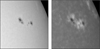 |
Fig. 1 Sample pair of WL and CaII-K segments used for whitelight-to-calcium translation. The segments in both modalities are spatially aligned and centered near an active region. |
2.1 Translation from WL to CaIIK images
We used observations recorded by the USET station located at ROB (Bechet & Clette 2002) and available within the SOLARNET Virtual Observatory (Mampaey et al. 2025). More precisely, we consider the dataset that simultaneously monitors the photosphere in WL and the lower chromosphere in CaIIK since 2012, encompassing a temporal range comparable to a full solar cycle. We selected daily pairs of (WL, CaIIK) images (size 2048 × 2048) through a careful process: highest-quality daily WL images are identified, then paired with the best available CaIIK images, minimizing the time difference between them. A maximum temporal difference of four hours is considered in order to avoid discrepancies due to too large displacements. For each pair, derotation was applied to co-align WL and CaIIK images using the SunPy module (The SunPy Community 2020) and a per-modality normalization is performed. The WL images were normalized using their maximum value, while CaIIK images are clipped at the 99.99th percentile and normalized using this value to account for potential flares. We note that the limb darkening was not corrected for either WL or CaIIK images, as this step would have little effect on the contrast between faculae and plage and quiet Sun regions, which are central to this translation task. The (WL, CaIIK) image pairs then underwent further processing: both modalities are scaled to the [−1,1] range, then the sub-image that is 512 × 512 in size, called ‘segments’, were extracted from the original full disk images. These segments were centered at sunspot locations, obtained from the USET sunspot group catalog table access protocol (TAP) service (Bechet & Clette 2024). When segments extended beyond the full-disk image boundaries, −1 padding was applied to fill the out-of-bound regions. Finally, to reduce computational cost, the segments were resized to 256 × 256 pixels. Figure 1 shows an example of (WL, CaIIK) segment pair.
2.2 Translation from EUV images to magnetograms
As a second application, our aim was to generate SDO/HMI magnetograms from EUV images captured by the Atmospheric Imaging Assembly (AIA) on board SDO (Lemen et al. 2012). We used the SDOMLv2 dataset1, which contains temporally and spatially aligned observations of SDO/AIA and SDO/HMI. The SDOMLv2 dataset is an updated version of the original SDOML dataset, described in Galvez et al. (2019). In this revision, the creators added observations up to the year 2020, changed the resolution of the images to 512 × 512 pixels and updated the data to account for change in calibration of the instruments.
Our goal was to perform translation of AIA images in the 304 Å bandpass (further denoted AIA-304 Å) to line-of-sight (LOS) magnetograms provided by HMI (simply denoted HMI). To reduce sample redundancy, the original cadences of AIA-304 Å (resp. HMI) images were reduced from six (resp. 12) minutes to four hours. We considered the central portion of the image, that is, a central segment of size 256 × 256 of the full-disk image. An example of AIA-304 Å and HMI pair is shown on Figure 2. In preprocessing, the intensities of AIA-304 Å images measured in digital number per second (DN/s) were clipped within the [0 DN/s, 1000 DN/s] range. This maximum value of 1000 DN/s was set to be above the 99.99th percentile of 100 randomly selected images. Analogously, the HMI LOS magnetic field measurements in Gauss (G) were clipped in the [−1500 G, 1500 G] interval. As with the previous task, both modalities are scaled to the [−1,1] range when used as input and target for the translation models.
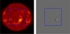 |
Fig. 2 Sample pair of AIA-304 Å and HMI images used for EUV-tomagnetogram translation. Only the central 256 × 256 pixels region is considered. |
3 Methods
This section presents two main strategies for translating images. We first adopted the conditional adversarial network approach introduced in Isola et al. (2017). It employs a conventional U-Net architecture, trained using an adversarial strategy and augmented with additional losses aimed at maximizing similarity between real and predicted images, as recommended by the Pix2PixCC model. Our experiments reveal that whilst popular, this model results in a significant amount of hallucinations.
Second, we envisioned non-adversarial strategies, starting with a variant of Pix2PixCC that omits the adversarial loss during training. Then, we explored a new method, which goes one step beyond adversarial loss removal to mitigate hallucinations. It questions the network architecture and proposes an extension of the convolutional blocks to incorporate input-dependent guidance in the image-to-image translation process through input-dependent modulation of the feature maps, following the principles of FiLM. For each input image, a guidance vector was extracted using a neural network and its components were linearly combined with U-Net feature maps. In practice, the parameters of the neural network in charge of extracting the guidance vector were learned during training.
In the rest of this section, without any loss of generality, the notations are based on the WL to CaIIK translation use case. Hence, we denote a pair of corresponding input-output samples as 𝒫 = (ℐ𝒲, ℐ𝒞), where ℐ𝒲 is the WL image and ℐ𝒞 is the view of the corresponding CaIIK image. The reconstruction of the CaIIK image estimated by the deep learning models is denoted ![Mathematical equation: $\[\widehat{\mathcal{I}}_{\mathcal{C}}\]$](/articles/aa/full_html/2025/10/aa55324-25/aa55324-25-eq1.png) .
.
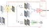 |
Fig. 3 Diagram of Pix2PixCC model and adversarial training for WL-to-CaIIK translation. The generator, G, converts a WL image to the CaIIK modality, the discriminator, D, distinguishes original WL-CaIIK pairs from forged pairs. The inspector(s) contributes to the update of the weights of G by computing correlation coefficients between the original CaIIK image and forged CaIIK image, at multiple scales. |
3.1 Conditional adversarial network
The Pix2PixCC model used in this work and its adversarial training are depicted in Figure 3. Pix2PixCC is composed of two sub-networks trained simultaneously: a generator, G, and a discriminator, D. Here, G is a CNN shaped according to the U-Net architecture. It is given a white light view, ℐ𝒲, and outputs an estimation of the corresponding calcium view, ![Mathematical equation: $\[\widehat{\mathcal{I}}_{\mathcal{C}}\]$](/articles/aa/full_html/2025/10/aa55324-25/aa55324-25-eq2.png) = G(ℐ𝒲). The generator is trained to make it close to the original ℐ𝒞, when available. In addition, the discriminator, D, is given a pair of images that can either be the original pair, 𝒫, or the forged pair,
= G(ℐ𝒲). The generator is trained to make it close to the original ℐ𝒞, when available. In addition, the discriminator, D, is given a pair of images that can either be the original pair, 𝒫, or the forged pair, ![Mathematical equation: $\[\widehat{\mathcal{P}}=(\mathcal{I}_{\mathcal{W}}, \widehat{\mathcal{I}}_{\mathcal{C}})\]$](/articles/aa/full_html/2025/10/aa55324-25/aa55324-25-eq3.png) . The role of D is to distinguish real pairs from the forged ones. It is implemented as a patchGAN (Isola et al. 2017) that manipulates pairs of patches (cropped in the pair of full images) instead of the image pair itself.
. The role of D is to distinguish real pairs from the forged ones. It is implemented as a patchGAN (Isola et al. 2017) that manipulates pairs of patches (cropped in the pair of full images) instead of the image pair itself.
During training, G is updated to improve the ability to fool D using a weighted sum of three loss functions: (a) the least-squares adversarial loss function for generators (Mao et al. 2017); (b) a feature-matching (FM) loss between ![Mathematical equation: $\[\widehat{\mathcal{I}}_{\mathcal{C}}\]$](/articles/aa/full_html/2025/10/aa55324-25/aa55324-25-eq4.png) and ℐ𝒞; and (c) a correlation coefficient based loss. We denote function (a) as ℒLS GAN, G and express it as
and ℐ𝒞; and (c) a correlation coefficient based loss. We denote function (a) as ℒLS GAN, G and express it as
![Mathematical equation: $\[\begin{aligned}\mathcal{L}_{L S~ G A N,~ G}(G, D) & =\frac{1}{2}\left(D\left(\mathcal{I}_\mathcal{W}, G\left(\mathcal{I}_\mathcal{W}\right)\right)-1\right)^2 \\& =\frac{1}{2}\left(D\left(\mathcal{I}_\mathcal{W}, \widehat{I}_\mathcal{C}\right)-1\right)^2,\end{aligned}\]$](/articles/aa/full_html/2025/10/aa55324-25/aa55324-25-eq5.png) (1)
(1)
where D(x, y) denotes the average of the real-or-fake results computed on patches pairs by the discriminator. It is considered as a probability, taking value of 0 if the input is detected as a forged pair and 1 if it is considered as a real pair by the discriminator. Loss (b), denoted ℒFM, takes the similarity between the reconstructed image and the target image into account to improve the reconstruction accuracy, expressed as
![Mathematical equation: $\[\mathcal{L}_{F M}(G, D)=\sum_{i=1}^{T_D} \frac{1}{N_i}\left\|D^{(i)}\left(\mathcal{I}_\mathcal{W}, \mathcal{I}_\mathcal{C}\right)-D^{(i)}\left(\mathcal{I}_\mathcal{W}, G\left(\mathcal{I}_\mathcal{W}\right)\right)\right\|,\]$](/articles/aa/full_html/2025/10/aa55324-25/aa55324-25-eq6.png) (2)
(2)
where TD is the number of layers in the discriminator, Di is the i-th layer of D, and Ni is the size of the feature map at the i-th layer. Finally, the loss (c) can be expressed as
![Mathematical equation: $\[\mathcal{L}_{C C}(G)=\sum_{i=0}^{T_{\downarrow}} \frac{1}{T_{\downarrow}+1}\left(1-C C_i\left(\mathcal{I}_\mathcal{C}, \widehat{I}_\mathcal{C}\right)\right),\]$](/articles/aa/full_html/2025/10/aa55324-25/aa55324-25-eq7.png) (3)
(3)
where CCi is the correlation coefficient measured at the i-th level of downsampling of ![Mathematical equation: $\[\widehat{\mathcal{I}}_{\mathcal{C}}\]$](/articles/aa/full_html/2025/10/aa55324-25/aa55324-25-eq8.png) and ℐ𝒞, and T↓ is the number of downsampling by a factor of two. The total loss minimized during the training of the generator in the Pix2PixCC framework is expressed as
and ℐ𝒞, and T↓ is the number of downsampling by a factor of two. The total loss minimized during the training of the generator in the Pix2PixCC framework is expressed as
![Mathematical equation: $\[\mathcal{L}_{t o t, G}(G, D)=\lambda_1 \mathcal{L}_{L S~ G A N, ~G}(G, D)+\lambda_2 \mathcal{L}_{F M}(G, D)+\lambda_3 \mathcal{L}_{C C}(G),\]$](/articles/aa/full_html/2025/10/aa55324-25/aa55324-25-eq9.png) (4)
(4)
with λ1, λ2 and λ3 being hyperparameters defining the relative importance of the sub-losses. In our experiments, we used λ1 = 2, λ2 = 5 and λ3 = 10. Concurrently, D was modified to improve its ability to distinguish between real and fake pairs using the least-square GAN loss function for discriminators, expressed as
![Mathematical equation: $\[\mathcal{L}_{L S~ G A N, ~D}(G, D)=\frac{1}{2}\left(D\left(\mathcal{I}_\mathcal{W}, \mathcal{I}_\mathcal{C}\right)-1\right)^2+\frac{1}{2}\left(D\left(\mathcal{I}_\mathcal{W}, G\left(\mathcal{I}_\mathcal{W}\right)\right)\right)^2.\]$](/articles/aa/full_html/2025/10/aa55324-25/aa55324-25-eq10.png) (5)
(5)
3.2 Non-adversarial strategies
The adversarial setup of GAN models often generates outputs with hallucinations, or unwanted artifacts. To mitigate this issue in our physics-sensitive application, we tested several approaches, described below.
3.2.1 Pix2PixCC without adversarial loss
We use Pix2Pixw/o-Adv to denote a variant of Pix2PixCC trained without adversarial loss or feature modulation and utilizing an L1 loss between the reconstruction and the target,
![Mathematical equation: $\[\mathcal{L}_{\mathrm{w} / \mathrm{o}-\mathrm{Adv}, G}=\left\|\mathcal{I}_\mathcal{C}-\widehat{I}_\mathcal{C}\right\|_1=\frac{1}{N_p} \sum_i^{N_p}\left|\widehat{I}_{C, i}-I_{C, i}\right|,\]$](/articles/aa/full_html/2025/10/aa55324-25/aa55324-25-eq11.png) (6)
(6)
where Np is the number of pixels in images.
3.2.2 Modulation of internal feature maps: I2IwFILM
To further mitigate unwanted artifacts, we propose an alternative approach that utilizes an I2I translation model with enhanced capacity to adapt the output reconstruction to the input content. This network uses FiLM layers to modulate its internal feature maps via learned affine transformations, thereby offering it the ability to inject input-related information through the image translation process. When the modulation factors are derived from the input signal this enables flexible task adaptation to this input. FiLM has been used across various tasks, from visual reasoning (Perez et al. 2017) to image translation (Park et al. 2019; Asensio Ramos et al. 2022; Huang & Belongie 2017). To our knowledge, the principles of FiLM have rarely been considered in solar physics research. In Asensio Ramos et al. (2022), FiLM layers have been used to generate surface temperature maps of stars, conditioned on the available observational phases. In the context of ground-based solar observations, which are often disturbed by Earth’s atmospheric effects, Asensio Ramos (2024) has proposed a CNN to emulate a spatially variant convolution with a point spread function (PSF), and uses FiLM layers to condition this convolution on the ground based instrument’s characteristics.
Formally, image-to-image translation with feature-wise linear modulation (I2IwFiLM) was implemented as depicted in Figure 4. To increase the chance that the guidance vector would capture information that is relevant to the output, in a preliminary training stage, the guidance vector, ℰ𝒫, was defined on the basis of the complete WL and CaIIK pair, 𝒫. Specifically, an encoding convolutional neural network called a GVP𝒫 (from guidance vector prediction) network was trained to extract a 256-dimensional guidance vector ℰ𝒫 from the concatenated input and output signals. The guidance vector ℰ𝒫 modulates the output of several convolutional layers in the main U-Net through dedicated linear layers. Each modulated convolutional layer is paired with its own linear layer, which takes ℰ𝒫 as its input and produces an additive modulation signal that is combined with the convolutional layer’s output (see Figure 4b). The number of channels of each linear layer output matches that of its associated feature map at the given depth of the main model. During the modulation, each element of the linear layer output is broadcast spatially across its corresponding H × W channel slice. Then, in a second step, another CNN is trained to predict the guidance vector ℰ𝒫 from the input signal only. The second training step is depicted in Figure 5. Analogously to the first training stage, the network trained to predict ℰ𝒫 from the sole WL image is denoted GVP𝒲. During this second stage, the main U-Net is refined, allowing it to adapt to the inaccuracies of GVP𝒲 approximating the behavior of GVP𝒫, while maintaining the reconstruction optimization.
The idea of training a FiLM guidance vector generator in two steps was initially introduced in Xia et al. (2023, 2025) to deal with image-to-image tasks corresponding to super-resolution, deblurring, and inpainting (but not cross-modal image translation). However, in contrast to our approach, as described in Appendix A, DiffI2I (Xia et al. 2025) uses a diffusion model to generate the guidance vector from a noise sample through a conditional denoising process. We recommend a straightforward prediction of the guidance vector using a feed-forward multilayer perceptron (MLP), without resorting to a diffusion process. In that way, we were able to avoid introducing randomness (through the diffusion process random seed) when computing the guidance vector, making the image translation deterministic. Our experiments demonstrate the relevance of our approach.
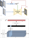 |
Fig. 4 First training stage of I2IwFiLM: a) Main U-Net model predicts |
![Mathematical equation: $\[\widehat{\mathcal{I}}_{\mathcal{C}}\]$](/articles/aa/full_html/2025/10/aa55324-25/aa55324-25-eq12.png)
![Mathematical equation: $\[\widehat{\mathcal{I}}_{\mathcal{W}}\]$](/articles/aa/full_html/2025/10/aa55324-25/aa55324-25-eq13.png)
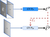 |
Fig. 5 Second training stage of I2IwFiLM. GVP𝒲, composed of convolutional layers followed by a MLP, learns to recover ℰ𝒫 vectors directly from ℐ𝒲. GVP𝒫 (dark blue) is frozen during this stage, while the main U-Net is left unconstrained to adapt to discrepancies due to guidance modification. |
4 Experiments
Our experiments investigate deep learning models trained with or without adversarial loss, both with and without input-dependent feature modulation for two I2I translation tasks. To evaluate how adversarial training and feature modulation impact physics-sensitive translation, we compared three models:
Pix2PixCC as proposed by Jeong et al. (2022), serving as the baseline model.
Pix2Pixw/o-Adv, a variant of Pix2PixCC trained without adversarial loss, utilizing an L1 loss between the reconstruction and the target.
I2IwFiLM, implementing feature modulation through input-dependent guidance
![Mathematical equation: $\[\widehat{\mathcal{E}^{\mathcal{P}}}\]$](/articles/aa/full_html/2025/10/aa55324-25/aa55324-25-eq14.png) , directly predicted from WL only. The training of this model minimizes L1 loss for both translation (reconstruction vs. target) and
, directly predicted from WL only. The training of this model minimizes L1 loss for both translation (reconstruction vs. target) and ![Mathematical equation: $\[\widehat{\mathcal{E}^{\mathcal{P}}}\]$](/articles/aa/full_html/2025/10/aa55324-25/aa55324-25-eq15.png) prediction.
prediction.
Section 4.1 details the train-test split adopted for both translation tasks. Model evaluation metrics are detailed in Section 4.2.
4.1 Train-test data splitting
To create the test sets of our two translation tasks, two months were selected from each year for both datasets: one winter month and one summer month, to ensure sample diversity. All samples corresponding to these selected months were allocated to the respective test sets. All other samples were selected for training, except the ones falling within a 12-day window on either side of the test samples. The window size was chosen as half of the Sun’s rotation period, as observed by Jha et al. (2021).
This results in a WL-to-CaIIK translation dataset including 6387 samples for training and 1410 for testing. For the AIA-304 Å-to-HMI translation, the number of samples is 17 072 for training and 3220 for testing.
4.2 Performance metrics
Our image-to-image translation models were evaluated at two distinct levels: generic image reconstruction level and application-specific level. The generic evaluation was performed using metrics detailed in Section 4.2.1, while the applicationspecific performance assessment was performed using metrics presented in Section 4.2.3 for AIA304 Å-to-HMI translation and in Section 4.2.2 for WL-to-CaIIK.
4.2.1 General metrics
We compared the reconstruction performance of the deep learning models using metrics that are common in the context of image reconstruction. We used the root mean square error (RMSE), peak signal-to-noise ratio (PS/N), structure similarity index measure (SSIM), and its extension: the multi-scale structure similarity index measure (MS-SSIM). Detailed descriptions of these metrics are given in Appendix B.
4.2.2 Metrics specific to the WL-to-CaIIK application
In the context of WL-to-CaIIK, a physically relevant metric consists of measuring the capacity of the models to reconstruct the plages and extended network of the target calcium image. To do so, we compared the plage segmentation masks computed from the original CaIIK and from the calcium images generated from WL. The masks are defined on full-disk images where the center-to-limb brightness variation was corrected. They include pixels brighter than a threshold defined as
![Mathematical equation: $\[\mu_{f d}+m * \sigma_{f d},\]$](/articles/aa/full_html/2025/10/aa55324-25/aa55324-25-eq16.png) (7)
(7)
where μfd is the mean brightness value of the full disk, σfd its standard deviation, and m a user-defined multiplicative factor, set to 4 in our experiments. We employed two metrics to compare the segmentation masks. First, the plage pixel ratio (PPR) is defined as the ratio of plage pixels in generated and original images. Second, the intersection over union (IoU) is computed as the ratio between the number of pixels that belong to both masks and the number of pixels that belong to at least one mask.
4.2.3 Metrics specific to the AIA-to-HMI application
In the context of AIA-to-HMI translation, HMI magnetograms exhibit bipolar pixel distributions centered at zero, with features of interest occupying a relatively small spatial extent. This characteristic poses challenges for conventional evaluation metrics such as SSIM, which may yield artificially elevated values due to large regions of zeros in reconstructed images, as observed by Dannehl et al. (2024). To mitigate this limitation, we introduce ΔSSIM, defined as the difference between two measures: (1) the SSIM between the generated and target magnetograms (SSIMmodel) and (2) a baseline SSIM computed between the target magnetogram and a reference image filled with zero values (SSIMflat). Formally, ΔSSIM is computed as
![Mathematical equation: $\[\Delta \mathrm{SSIM}=\mathrm{SSIM}_{model}-\mathrm{SSIM}_{flat}.\]$](/articles/aa/full_html/2025/10/aa55324-25/aa55324-25-eq17.png) (8)
(8)
This differential metric accounts for the inherent sparsity of magnetic features in HMI observations and enables a performance comparison focused on active regions.
5 Results
5.1 Generic reconstruction quality metrics
An overview of the reconstruction performance is given in Table 1 for WL-to-CaIIK and AIA304 Å-to-HMI translations. Based on this table, we can observe that removing adversarial training improves reconstruction performance: Pix2PixCCw/o-Adv outperforms Pix2PixCC across all generic metrics, suggesting non-adversarial training provides a stronger foundation for physics-sensitive I2I tasks. Furthermore, incorporating modulation based on FiLM principles further enhances translation quality, as evidenced by our proposed I2IwFiLM’s superior metrics over Pix2PixCCw/o-Adv. We interpret these results as a consequence of the input lacking complete information for perfect target reconstruction, as evidenced by spatial mismatches between WL faculae and CaIIK plages. While adversarial models such as Pix2PixCC produce visually compelling results by overinterpreting available data to match target distributions, this leads to hallucinations and lower reconstruction metrics.
In the remainder of this section, we analyze the performance of Pix2PixCC and I2IwFiLM across both image-to-image translation tasks. Section 5.2 presents a comparison of the models for the WL-to-CaIIK translation task, while Section 5.3 focuses on the AIA-304 Å-to-HMI translation.
5.2 WL-to-CaIIK
Figures 7 and 8 illustrate examples of white light to calcium modality translations at different locations on the solar disk. The former shows high-quality reconstructions, while the latter demonstrates subpar examples with additional physically inaccurate plage regions. These figures demonstrate typical model behaviors: Pix2PixCC, trained with adversarial setup, produces visually appealing results with high-frequency features, but exhibits a tendency to generate plage regions where there are none. This behavior is referred to as a “hallucination”. In contrast, I2IwFiLM generates outputs that appear blurrier but achieve more physically accurate reconstructions without hallucinations. Additionally, Figures 7 and 8 reveal the variations in translation quality with respect to the angular distance sin(θ) between solar center and sunspot location. The analysis of reconstruction metrics binned by sin(θ), presented in Figure 9, quantifies these variations. Two distinct regimes emerge in the translation quality: regions with sin(θ) < 0.6 show poor translation performance, while regions with sin(θ) > 0.6 exhibit increasingly accurate reconstructions as they approach the limb. Those two regimes are explained by Figure 6, which shows that in both input and output images, the contrast between features belonging to active regions (ARs) increases with sin(θ). Alongside sunspots, visible AR features are faculae in WL images, while the plage and extended network are visible in CaIIK images. Beyond the impact of sin(θ), Figure 9 also shows that I2IwFiLM consistently outperforms Pix2PixCC with respect to every metric across all angular distances bins.
Figure 10 evaluates the performance of our models using application-specific metrics. It presents histograms of PPR and IoU metrics on test set samples for 3 ranges of sin(θ): (a) the center of the Sun (0 ≤ sin(θ) ≤ .5), where faculae are indistinguishable from the background in WL images, (b) the transitional region (.5 ≤ sin(θ) ≤ .75), and (c) the region nearing the limb (.75 ≤ sin(θ) ≤ 1) with a high contrast between faculae and background. Both Pix2PixCC and I2IwFiLM models demonstrate improved reconstruction performance as sin(θ) increases, with higher mean PPR and IoU values and the reduction in their standard deviations. However, both models appear to be limited by the visibility of faculae, resulting in the production of plage regions smaller than the actual ones in the targets. This limitation is revealed by both PPR and IoU achieving their best values in the regions where faculae are most easily discernible. Examining the models individually, I2IwFiLM exhibits low average PPR and IoU with large variance for sin(θ) ≤ 0.5, indicating that only a fraction of plages in these active regions are consistently reconstructed, as observed in Figure 7 (top row) and Figure 8 (left). In contrast, Pix2PixCC achieves a respectable PPR but poor IoU for these regions, suggesting consistent incorrect reconstruction of plages due to hallucinations. When comparing the relative performance of the two models, it is noteworthy that the mean PPR of I2IwFiLM initially lags behind that of Pix2PixCC for sin(θ) ≤ .5 but surpasses it for sin(θ) > .75, accompanied by a substantial reduction in its standard deviation. Given these results, I2IwFiLM appears to be more suitable for white light-to-calcium translation compared to Pix2PixCC.
These results illustrate the possibility of reconstructing CaIIK plages from faculae observed in WL when these are located at an angular distance of about 40 degrees or more from the disk center. In future works, these generated images could be compared to observations from a data archive to help remove inconsistencies these historical archive might have (Chatzistergos et al. 2024). However, to reconstruct solar irradiance at the CaIIK line, we would need to obtain information also at smaller angular distances. This would require to process not only a single image, but a time series of observations, to allow the transfer of information from one timestamp to another.
Performance comparison with respect to generic image reconstruction metrics.
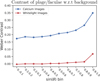 |
Fig. 6 Weber contrast between foreground and background pixels intensity along angular distance bins in WL and CaIIK images. The Weber contrast is defined as the ratio of luminance difference between foreground and background over the background luminance (see Appendix C). The quiet Sun is considered background while foreground is the combination of plage and extended network in CaIIK images, and faculae in WL. |
5.3 AIA-304 Å-to-HMI
An example of AIA-304 Å-to-HMI translation is depicted in Figure 11. As observed for WL-to-CaIIK translation, Pix2PixCC generates visually more appealing images than I2IwFiLM, but hallucinations degrade quantitative results. The example illustrates that flat HMI images inherently share high metric values when compared with target images, making a fair comparison between the models challenging.
Both models accurately locate the active regions. They also had the capability to infer Hale’s law during training and reproduce the leading polarity accurately in their output, but failed at outlining details of active regions from AIA-304 Å images. Indeed, the active regions in the generated images only faintly correspond to the target, as indicated by the SSIM maps.
To assess the application-specific performance, we introduce the ΔSSIM metric in Section 4.2.3. Computed on the entire image, it evaluates whether translation models outperform a trivial zero-image baseline. The left part of Figure 12 shows histograms of ΔSSIM metrics of all test samples for both Pix2PixCC and I2IwFiLM models. The histogram for Pix2PixCC (μ = −0.019, σ = 0.0096) lies entirely on the left of the vertical line at ΔSSIM = 0, indicating that Pix2PixCC’s reconstructions correspond to the target even less than a flat HMI image due to the hallucination it generates. In contrast, the histogram of I2IwFiLM (μ = 0.0053, σ = 0.0052) is positioned on the right of the line, demonstrating that I2IwFiLM performs better than a zero-constant reconstruction of the target.
To further investigate the reconstruction quality of active regions, we computed the same ΔSSIM histograms at the active region level. To do so, crops of ARs were extracted from test samples and ΔSSIM metrics were computed over those crops. Only active regions of classes C and larger according to the modified Zurich classification scheme (McIntosh 1990) were considered in this analysis, while small-sized active regions were excluded. The classes of active regions were obtained from the USET sunspot groups catalog (Bechet & Clette 2024). The resulting ΔSSIM histograms for active regions are shown in the right part of Figure 12. By focusing solely on the sparse ARs, the histograms become more widely distributed compared to the full-image analysis. This widening occurs because the results in ARs are less diluted by the overall good performance in the large zero-valued regions, which typically cause the histograms obtained on entire images to become narrower, while shifting them closer to zero. The observations made for the full-image analysis still hold: the positive average of I2IwFiLM’s histogram (μ = 0.0293) with a narrow standard deviation (σ = 0.0293) and the negative average of Pix2PixCC’s histogram (μ = −0.0119) with a higher standard deviation (σ = 0.0375) shows that the hallucinations produced by Pix2PixCC make it less suitable for physically accurate image translation than I2IwFiLM.
In future works, the reconstruction with I2IwFiLM could be further improved by constraining more the target modality using multidimensional input images. For example, in the generation of magnetogram from EUV images, the input used by Jeong et al. (2022) included the EUV information, along with some reference data pairs. During training, the EUV information consists of three SDO/AIA channels at time of interest and the reference data pair is composed of three SDO/AIA images and an SDO/HMI magnetogram, which were observed over one solar rotation prior to the time of interest. In the prediction phase, the algorithm inputs the three STEREO-EUVI channels (for which the corresponding magnetogram must be generated) and the reference data pairs were built using the latest corresponding SDO data; namely, the frontside data selected by considering the separation angle between STEREO and SDO spacecrafts. In other words, it is expected that the frontside magnetograms will constrain the model with information about the overall magnetic field distribution. More scientific validation could also be provided by comparing the predictions of solar wind simulation models obtained with either AI-generated or original magnetograms used as boundary conditions, as explored by Li et al. (2024).
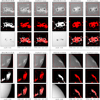 |
Fig. 7 Highest-quality CaIIK reconstructions of ARs near the center of the solar disk (top) and near the limb (bottom). In each 3 × 3 grid, the top row shows the original CaIIK image (left) and its reconstructions by I2IwFiLM (middle) and Pix2PixCC (right). The middle row shows segmentation masks of plages visible in the original CaIIK image (left) and the corresponding reconstructions by I2IwFiLM (middle) and Pix2PixCC (right). Bottom row shows input white light (WL) image (left) and overlays of the target plage mask with the model-generated plage masks from I2IwFiLM (middle) and Pix2PixCC (right), facilitating a direct comparison. The red square corresponds to the sub-image provided as input to the models; a slightly larger image is shown to indicate the consistency with the surroundings. |
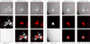 |
Fig. 8 Subpar CaIIK reconstructions of ARs near the center of the solar disk (left grid) and near the limb (right grid). In each 3 × 3 grid: the top row shows the original CaIIK image (left) and its reconstructions by I2IwFiLM (middle) and Pix2PixCC (right). The middle row shows segmentation masks of plages visible in the original CaIIK image (left) and the corresponding reconstructions by I2IwFiLM (middle) and Pix2PixCC (right). Bottom row shows input white light (WL) image (left) and overlays of the target plage mask with the model-generated plage masks from I2IwFiLM (middle) and Pix2PixCC (right), facilitating a direct comparison. |
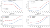 |
Fig. 9 Comparison of Pix2PixCC and I2IwFiLM performances using generic image reconstruction metrics along the angular distance bins to the center of the Sun. The center of the Sun corresponds to sin(θ) = 0, while the limb corresponds to sin(θ) = 1. |
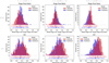 |
Fig. 10 Plage reconstruction performance of Pix2PixCC and I2IwFiLM models for active regions located near the center of the sun (left column), at intermediate distance to the center (middle column), and near the limb (right column). Top row shows PPR metric histograms. Bottom row shows intersection over union (IoU) histograms. |
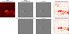 |
Fig. 11 Example of reconstructed HMI Bz using Pix2PixCC model (GAN-based) and I2IwFiLM (ours). From left to right: Input AIA-304 Å image, target HMI image compared with flat HMI, model-reconstructed HMI images, and structure similarity maps between model-reconstructed HMI and target. |
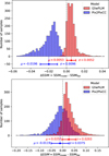 |
Fig. 12 ΔSSIM histograms for I2IwFiLM and Pix2PixCC models computed on images in AIA-304 Å-to-HMI task test set. Top: Entire images. Bottom: Crops centered on large ARs only (McIntosh class C and larger). |
6 Discussion and conclusions
Solar physics benefits from continuously evolving observational capabilities that provide new measurement modalities. However, in some cases, modern observations were not available in the past, creating gaps in historical data, or they might not be taken from the desired vantage point, causing inaccuracy in physical models that input them as boundary conditions. We leveraged deep learning methods to reconstruct these missing modalities from physically related measurements that were available at the time of interest. For such reconstructions, GANs have become the standard approach.
In this work, we address two translation tasks in solar physics: WL-to-CaIIK and EUV-to-magnetogram. Unlike traditional image reconstruction tasks (e.g., super-resolution) where the input contains most of the target information, the modalities involved in our cross-modal translation tasks generally share only a fraction of their respective visual cues. This lack of guidance makes GANs prone to hallucinations, driven by the need to match target modality statistics, a critical flaw in scientific applications. Therefore, we propose a novel deep learning approach named I2IwFiLM that replaces adversarial training by enhanced guidance from input modalities. I2IwFiLM relies on a side model to extract information from the input and modulate the feature maps of the main translation model. This design preserves information content while benefiting from non-adversarial training to reduce hallucinations. Our study shows that while methods based on GANs produce more visually attractive results, I2IwFiLM generates images closer to the target images, with better reconstruction metrics. To rigorously assess and compare their respective physical relevance, we introduced domain-specific metrics for both WL-to-CaIIK and EUV-tomagnetogram tasks. The evaluations demonstrate superior performance for our I2IwFiLM method, across these metrics.
The approach presented in this work allows for physically accurate reconstruction of missing solar observations, providing exploitable data for downstream space weather and solar physics research. In the future, follow-up works could explore fine-tuning the translation models by exploiting plage masks-related metrics such as PPR and IoU directly into the training loss. Further improvements of the methods could also be achieved by using multidimensional input, either from time-series or multiple channel observations. Further scientific validation could also involve the use of generated images as boundary conditions in a physical simulation, along with a comparison of the quality of the resulting simulation output.
Data availability
The data used for the WL-to-CaII K translation is freely available through the SOLARNET Virtual Observatory website: https://solarnet.oma.be/. The SDOMLv2 dataset used for the EUV-to-Magnetogram translation task can be found on github: https://github.com/SDOML/SDOMLv2. The code used for this work is also publicly available on github: https://github.com/sayez/I2IwFiLM.git.
Acknowledgements
We thank Jeong et al. for making the Pix2PixCC code available and Galvez et al. for their well-prepared machine learning dataset. We also thank all the team members of the SDO mission and acknowledge efforts supporting open-source solar data analysis Python packages we utilize in this work: NumPy, Matplotlib, PyTorch, SunPy, Astropy, and Aiapy. These results were obtained in the framework of the project B2/191/P2/DeepSun funded by the Belgian Federal Science Policy Office (BELSPO). Part of the work was sponsored by the Solar-Terrestrial Centre of Excellence, a collaboration between ROB, the Royal Meteorological Institute, and the Royal Belgian Institute for Space Aeronomy funded by BELSPO. Computational resources have been provided both by the supercomputing facilities of the UCLouvain (CISM/UCL) and the Consortium des Equipements de Calcul Intensif en Fedération Wallonie Bruxelles (CECI) funded by the Fond de la Recherche Scientifique de Belgique (F.R.S.-FNRS) under convention 2.5020.11 and by the Walloon Region.
Appendix A I2IwFiLM versus DiffI2I
In contrast to I2IwFiLM which uses a deterministic CNN to predict guidance vectors ![Mathematical equation: $\[\widehat{\mathcal{E}^{\mathcal{P}}}\]$](/articles/aa/full_html/2025/10/aa55324-25/aa55324-25-eq18.png) (see Figure 5), DiffI2I (Xia et al. 2025) adopts a diffusion-based process to generate the guidance vectors from random seeds. The training of this diffusion process is depicted in Figure A.1. CPEN𝒫 is a network with similar role as GVP𝒫 in Figure 4 and CPEN𝒲 learns an intermediate embedding space that influences the generation of guidance vectors using a diffusion model DM. During this training stage, the weights of both DM and CPEN𝒲 are updated using the L1 loss between the clean ε𝒫 (prior to forward diffusion) and its reconstruction
(see Figure 5), DiffI2I (Xia et al. 2025) adopts a diffusion-based process to generate the guidance vectors from random seeds. The training of this diffusion process is depicted in Figure A.1. CPEN𝒫 is a network with similar role as GVP𝒫 in Figure 4 and CPEN𝒲 learns an intermediate embedding space that influences the generation of guidance vectors using a diffusion model DM. During this training stage, the weights of both DM and CPEN𝒲 are updated using the L1 loss between the clean ε𝒫 (prior to forward diffusion) and its reconstruction ![Mathematical equation: $\[\widehat{\epsilon^{\mathcal{P}}}\]$](/articles/aa/full_html/2025/10/aa55324-25/aa55324-25-eq19.png) . Table A.1 compares translation performance of our proposed I2IwFiLM with DiffI2I using generic reconstruction metrics. These results demonstrate that the simplified network architecture of I2IwFiLM, which omits diffusion-based guidance vector generation, performs as effectively as the more complex design of DiffI2I for cross-domain image translation.
. Table A.1 compares translation performance of our proposed I2IwFiLM with DiffI2I using generic reconstruction metrics. These results demonstrate that the simplified network architecture of I2IwFiLM, which omits diffusion-based guidance vector generation, performs as effectively as the more complex design of DiffI2I for cross-domain image translation.
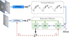 |
Fig. A.1 Second training stage of DiffI2I model learning to recover ℰ𝒫 vectors from embedding space ℰ𝒲. DiffI2I model uses forward and backward diffusion process for recovery. In contrast to our deterministic I2IwFiLM approach, involving noise introduces diversity in ℰ𝒫 recovery, potentially affecting physical accuracy of |
![Mathematical equation: $\[\widehat{\mathcal{I}}_{\mathcal{C}}\]$](/articles/aa/full_html/2025/10/aa55324-25/aa55324-25-eq20.png)
Quantitative comparison of I2IwFiLM and DiffI2I.
Appendix B Quality metrics
PS/N
The peak signal-to-noise ratio (PS/N) is defined as
![Mathematical equation: $\[\mathrm{PS} / \mathrm{N}=10 \cdot \log _{10}\left(\frac{\max \left(I_C\right)^2}{\operatorname{MSE}\left(\mathcal{I}_\mathcal{C}, \widehat{\mathcal{I}}_\mathcal{C}\right)}\right)\]$](/articles/aa/full_html/2025/10/aa55324-25/aa55324-25-eq22.png) (B.1)
(B.1)
where max(IC) is the maximum possible pixel value in IC and MSE is the mean square error.
SSIM and MS-SSIM
Structure similarity index measure (SSIM, Wang et al. 2004) is a perceptual metric that evaluates image similarity by comparing structural information between an image and a reference, which captures luminance l, contrast c and the spatial dependencies s of pixels. The complete SSIM metric is expressed as follows:
![Mathematical equation: $\[\begin{aligned}\operatorname{SSIM}\left(\mathcal{I}_\mathcal{C}, \widehat{\mathcal{I}}_\mathcal{C}\right) & =l\left(\mathcal{I}_\mathcal{C}, \widehat{\mathcal{I}}_\mathcal{C}\right) \cdot c\left(\mathcal{I}_\mathcal{C}, \widehat{\mathcal{I}}_\mathcal{C}\right) \cdot s\left(\mathcal{I}_\mathcal{C}, \widehat{\mathcal{I}}_\mathcal{C}\right) \\& =\frac{\left(2 \mu_{\mathcal{I}_\mathcal{C}} \mu_{\widehat{\mathcal{I}}_\mathcal{C}}+k_1 L\right)\left(2 \sigma_{\widehat{\mathcal{I}}_\mathcal{C} \mathcal{I}_\mathcal{C}}+k_2 L\right)}{\left(\mu_{\mathcal{I}_\mathcal{C}}^2+\mu_{\widehat{\mathcal{I}}_\mathcal{C}}^2+k_1 L\right)\left(\sigma_{\mathcal{I}_\mathcal{C}}^2+\sigma_{\widehat{\mathcal{I}}_\mathcal{C}}^2+k_2 L\right)},\end{aligned}\]$](/articles/aa/full_html/2025/10/aa55324-25/aa55324-25-eq23.png) (B.2)
(B.2)
where μℐ𝒞, σℐ𝒞 (resp. ![Mathematical equation: $\[\mu_{\widehat{\mathcal{I}}_{\mathcal{C}}}, \sigma_{\widehat{\mathcal{I}}_{\mathcal{C}}}\]$](/articles/aa/full_html/2025/10/aa55324-25/aa55324-25-eq24.png) ) are the mean and standard deviation of the target (resp. generated) calcium image,
) are the mean and standard deviation of the target (resp. generated) calcium image, ![Mathematical equation: $\[\sigma_{\widehat{\mathcal{I}}_{\mathcal{C}} \mathcal{I}_{\mathcal{C}}}\]$](/articles/aa/full_html/2025/10/aa55324-25/aa55324-25-eq25.png) denotes the covariance between the covariance between
denotes the covariance between the covariance between ![Mathematical equation: $\[\widehat{\mathcal{I}}_{\mathcal{C}}\]$](/articles/aa/full_html/2025/10/aa55324-25/aa55324-25-eq26.png) and ℐ𝒞. Finally, L denotes the dynamic range of the pixel values and k1, k2 are constants ensuring non-zero denominators.
and ℐ𝒞. Finally, L denotes the dynamic range of the pixel values and k1, k2 are constants ensuring non-zero denominators.
An extension of SSIM metric, named multi-scale SSIM (MS-SSIM, see Wang et al. 2003), was introduced to enhance its quality by taking the multi-scale nature of the human vision into account in its computation. Both reference and generated images are downscaled to lower resolution such that the luminance, contrast and structure elements of the SSIM can be computed at every scale level. The final MS-SSIM is obtained by multiplying the luminance comparison of the lowest downsampling level with the cumulated product of the contrast and structure comparisons of every down sampling level. Formally, the MS-SSIM is computed as follows
![Mathematical equation: $\[\operatorname{MS-SSIM}(\mathcal{I}_\mathcal{C}, \widehat{I}_\mathcal{C})=l_m(\mathcal{I}_\mathcal{C}, \widehat{I}_\mathcal{C}) \cdot \prod_{j=1}^m[c_j(\mathcal{I}_\mathcal{C}, \widehat{I}_\mathcal{C}) \cdot s_j(\mathcal{I}_\mathcal{C}, \widehat{I}_\mathcal{C})],\]$](/articles/aa/full_html/2025/10/aa55324-25/aa55324-25-eq27.png) (B.3)
(B.3)
where m denotes the maximum downsampling level and cj, sj, and lj denote the contrast, luminance, and structure comparisons, respectively, of the inputs scaled down to the jth level.
Appendix C Weber contrast
The Weber contrast (C) is defined as the ratio of luminance difference between foreground and background over the background luminance. In this work, the quiet Sun is considered as background, while the foreground is defined as the combination of plage in active regions and extended network in CaIIK images and faculae in WL images. Weber contrast (C) is expressed as.
![Mathematical equation: $\[C=\frac{\mu_{A R}-\mu_{b g}}{\mu_{b g}},\]$](/articles/aa/full_html/2025/10/aa55324-25/aa55324-25-eq28.png) (C.1)
(C.1)
where μAR is the average luminance of pixels in active regions, namely, plage or extended network in CaIIK and faculae in WL, and μbg is the average luminance of quiet Sun pixels.
References
- Amar, E., & Ben-Shahar, O. 2024, ApJS, 271, 29 [Google Scholar]
- Asensio Ramos, A. 2024, A&A, 688, A88 [NASA ADS] [CrossRef] [EDP Sciences] [Google Scholar]
- Asensio Ramos, A., Díaz Baso, C. J., & Kochukhov, O. 2022, A&A, 658, A162 [NASA ADS] [CrossRef] [EDP Sciences] [Google Scholar]
- Bechet, S., & Clette, F. 2002, USET images/L1-centered, https://doi.org/10.24414/nc7j-b391 [Google Scholar]
- Bechet, S., & Clette, F. 2024, USET Sunspot Group catalog, Table Access Protocol service available at http://vo-tap.oma.be/ [Google Scholar]
- Chatzistergos, T., Krivova, N. A., & Yeo, K. L. 2023, J. Atmos. Solar-Terrestrial Phys., 252, 106150 [Google Scholar]
- Chatzistergos, T., Krivova, N. A., & Ermolli, I. 2024, J. Space Weather Space Climate, 14, 9 [Google Scholar]
- Choi, J., Kim, S., Jeong, Y., Gwon, Y., & Yoon, S. 2021, in 2021 IEEE/CVF International Conference on Computer Vision (ICCV) (Los Alamitos, CA, USA: IEEE Computer Society), 14347 [Google Scholar]
- Cohen, O., Sokolov, I., Roussev, I., et al. 2006, ApJ, 654, L163 [Google Scholar]
- Creswell, A., White, T., Dumoulin, V., et al. 2018, IEEE Signal Process. Mag., 35, 53 [CrossRef] [Google Scholar]
- Dannehl, M., Delouille, V., & Barra, V. 2024, Earth Space Sci., 11, e2023EA002974 [Google Scholar]
- Galvez, R., Fouhey, D. F., Jin, M., et al. 2019, ApJS, 242, 7 [Google Scholar]
- Gao, F., Liu, T., Sun, W., & Xu, L. 2023, ApJS, 266, 19 [Google Scholar]
- Goodfellow, I., Pouget-Abadie, J., Mirza, M., et al. 2014, in Advances in Neural Information Processing Systems, 27, eds. Z. Ghahramani, M. Welling, C. Cortes, N. Lawrence, & K. Weinberger (Curran Associates, Inc.) [Google Scholar]
- Harvey, J. W., Hill, F., Hubbard, R. P., et al. 1996, Science, 272, 1284 [Google Scholar]
- Ho, J., Jain, A., & Abbeel, P. 2020, in Advances in Neural Information Processing Systems,33, eds. H. Larochelle, M. Ranzato, R. Hadsell, M. Balcan, & H. Lin (Curran Associates, Inc.), 6840 [Google Scholar]
- Howard, R. A., Moses, J. D., Vourlidas, A., et al. 2008, Space Sci. Rev., 136, 67 [NASA ADS] [CrossRef] [Google Scholar]
- Huang, X., & Belongie, S. 2017, in 2017 IEEE International Conference on Computer Vision (ICCV) (Los Alamitos, CA, USA: IEEE Computer Society), 1510 [Google Scholar]
- Isola, P., Zhu, J.-Y., Zhou, T., & Efros, A. A. 2017, in 2017 IEEE Conference on Computer Vision and Pattern Recognition (CVPR) (Los Alamitos, CA, USA: IEEE Computer Society), 5967 [Google Scholar]
- Jarolim, R., Veronig, A. M., Pötzi, W., & Podladchikova, T. 2025, Nat. Comm., 16, 3157 [Google Scholar]
- Jeong, H.-J., Moon, Y.-J., Park, E., & Lee, H. 2020, ApJ, 903, L25 [Google Scholar]
- Jeong, H.-J., Moon, Y.-J., Park, E., Lee, H., & Baek, J.-H. 2022, ApJS, 262, 50 [CrossRef] [Google Scholar]
- Jha, B. K., Priyadarshi, A., Mandal, S., Chatterjee, S., & Banerjee, D. 2021, Sol. Phys., 296, 25 [Google Scholar]
- Kim, T., Park, E., Lee, H., et al. 2019, Nat. Astron., 3, 397 [Google Scholar]
- Lawrance, B., Lee, H., Park, E., et al. 2022, ApJ, 937, 111 [Google Scholar]
- Lee, H., Park, E., & Moon, Y.-J. 2021, ApJ, 907, 118 [NASA ADS] [Google Scholar]
- Lemen, J. R., Title, A. M., Akin, D. J., et al. 2012, Sol. Phys., 275, 17 [Google Scholar]
- Li, X., Valliappan, S. P., Shukhobodskaia, D., et al. 2024, Space Weather, 22, e2023SW003499 [Google Scholar]
- Mampaey, B., Delouille, V., & Vansintjan, R. 2025, Sol. Phys., 300, 16 [Google Scholar]
- Mao, X., Li, Q., Xie, H., et al. 2017, in 2017 IEEE International Conference on Computer Vision (ICCV) (Los Alamitos, CA, USA: IEEE Computer Society), 2813 [Google Scholar]
- McIntosh, P. S. 1990, Sol. Phys., 125, 251 [NASA ADS] [CrossRef] [Google Scholar]
- Park, T., Liu, M.-Y., Wang, T.-C., & Zhu, J.-Y. 2019, in 2019 IEEE/CVF Conference on Computer Vision and Pattern Recognition (CVPR), 2332 [Google Scholar]
- Perez, E., Strub, F., Vries, H., Dumoulin, V., & Courville, A. 2017, Proc. AAAI Conf. Artif. Intell., 32 [Google Scholar]
- Pevtsov, A. A., Virtanen, I., Mursula, K., Tlatov, A., & Bertello, L. 2016, A&A, 585, A40 [NASA ADS] [CrossRef] [EDP Sciences] [Google Scholar]
- Pomoell, J., & Poedts, S. 2018, J. Space Weather Space Climate, 8, A35 [NASA ADS] [CrossRef] [EDP Sciences] [Google Scholar]
- Ramunno, F. P., Jeong, H.-J., Hackstein, S., et al. 2024, in Proceedings of SPAICE2024: The First Joint European Space Agency/IAA Conference on AI in and for Space, eds. D. Dold, A. Hadjiivanov, & D. Izzo, 75 [Google Scholar]
- Rochus, P., Auchère, F., Berghmans, D., et al. 2020, A&A, 642, A8 [NASA ADS] [CrossRef] [EDP Sciences] [Google Scholar]
- Rombach, R., Blattmann, A., Lorenz, D., Esser, P., & Ommer, B. 2022, in 2022 IEEE/CVF Conference on Computer Vision and Pattern Recognition (CVPR) (Los Alamitos, CA, USA: IEEE Computer Society), 10674 [Google Scholar]
- Ronneberger, O., Fischer, P., & Brox, T. 2015, in Medical Image Computing and Computer-Assisted Intervention – MICCAI 2015, eds. N. Navab, J. Hornegger, W. M. Wells, & A. F. Frangi (Cham: Springer International Publishing), 234 [Google Scholar]
- Saharia, C., Chan, W., Chang, H., et al. 2022, in ACM SIGGRAPH 2022 Conference Proceedings, SIGGRAPH’22 (New York, NY, USA: Association for Computing Machinery) [Google Scholar]
- Scherrer, P. H., Bogart, R. S., Bush, R. I., et al. 1995, Sol. Phys., 162, 129 [Google Scholar]
- Scherrer, P. H., Schou, J., Bush, R. I., et al. 2012, Sol. Phys., 275, 207 [Google Scholar]
- Shin, G., Moon, Y.-J., Park, E., et al. 2020, ApJ, 895, L16 [NASA ADS] [CrossRef] [Google Scholar]
- Shiota, D., & Kataoka, R. 2016, Space Weather, 14, 56 [CrossRef] [Google Scholar]
- Son, J., Cha, J., Moon, Y.-J., et al. 2021, ApJ, 920, 101 [NASA ADS] [CrossRef] [Google Scholar]
- Song, W., Ma, Y., Sun, H., Zhao, X., & Lin, G. 2024, A&A, 686, A272 [NASA ADS] [CrossRef] [EDP Sciences] [Google Scholar]
- Sun, W., Xu, L., Zhang, Y., Zhao, D., & Zhang, F. 2023, Res. Astron. Astrophys., 23, 025003 [Google Scholar]
- The SunPy Community (Barnes, W. T., et al.) 2020, ApJ, 890, 68 [Google Scholar]
- Vanden Broeck, G., Bechet, S., Clette, F., et al. 2024, A&A, 689, A95 [NASA ADS] [CrossRef] [EDP Sciences] [Google Scholar]
- Wang, T.-C., Liu, M.-Y., Zhu, J.-Y., et al. 2018, in 2018 IEEE/CVF Conference on Computer Vision and Pattern Recognition (CVPR) (Los Alamitos, CA, USA: IEEE Computer Society), 8798 [Google Scholar]
- Wang, Z., Simoncelli, E., & Bovik, A. 2003, in The Thirty-Seventh Asilomar Conference on Signals, Systems and Computers, 2, 1398 [Google Scholar]
- Wang, Z., Bovik, A. C., Sheikh, H. R., & Simoncelli, E. P. 2004, IEEE Trans. Image Process., 13, 600 [Google Scholar]
- Xia, B., Zhang, Y., Wang, S., et al. 2023, in 2023 IEEE/CVF International Conference on Computer Vision (ICCV) (Los Alamitos, CA, USA: IEEE Computer Society), 13049 [Google Scholar]
- Xia, B., Zhang, Y., Wang, S., et al. 2025, IEEE Trans. Pattern Anal. Mach. Intell., 47, 1578 [Google Scholar]
Available at https://github.com/SDOML/SDOMLv2
All Tables
All Figures
|
Fig. 1 Sample pair of WL and CaII-K segments used for whitelight-to-calcium translation. The segments in both modalities are spatially aligned and centered near an active region. |
| In the text | |
|
Fig. 2 Sample pair of AIA-304 Å and HMI images used for EUV-tomagnetogram translation. Only the central 256 × 256 pixels region is considered. |
| In the text | |
|
Fig. 3 Diagram of Pix2PixCC model and adversarial training for WL-to-CaIIK translation. The generator, G, converts a WL image to the CaIIK modality, the discriminator, D, distinguishes original WL-CaIIK pairs from forged pairs. The inspector(s) contributes to the update of the weights of G by computing correlation coefficients between the original CaIIK image and forged CaIIK image, at multiple scales. |
| In the text | |
|
Fig. 4 First training stage of I2IwFiLM: a) Main U-Net model predicts |
| In the text | |
|
Fig. 5 Second training stage of I2IwFiLM. GVP𝒲, composed of convolutional layers followed by a MLP, learns to recover ℰ𝒫 vectors directly from ℐ𝒲. GVP𝒫 (dark blue) is frozen during this stage, while the main U-Net is left unconstrained to adapt to discrepancies due to guidance modification. |
| In the text | |
|
Fig. 6 Weber contrast between foreground and background pixels intensity along angular distance bins in WL and CaIIK images. The Weber contrast is defined as the ratio of luminance difference between foreground and background over the background luminance (see Appendix C). The quiet Sun is considered background while foreground is the combination of plage and extended network in CaIIK images, and faculae in WL. |
| In the text | |
|
Fig. 7 Highest-quality CaIIK reconstructions of ARs near the center of the solar disk (top) and near the limb (bottom). In each 3 × 3 grid, the top row shows the original CaIIK image (left) and its reconstructions by I2IwFiLM (middle) and Pix2PixCC (right). The middle row shows segmentation masks of plages visible in the original CaIIK image (left) and the corresponding reconstructions by I2IwFiLM (middle) and Pix2PixCC (right). Bottom row shows input white light (WL) image (left) and overlays of the target plage mask with the model-generated plage masks from I2IwFiLM (middle) and Pix2PixCC (right), facilitating a direct comparison. The red square corresponds to the sub-image provided as input to the models; a slightly larger image is shown to indicate the consistency with the surroundings. |
| In the text | |
|
Fig. 8 Subpar CaIIK reconstructions of ARs near the center of the solar disk (left grid) and near the limb (right grid). In each 3 × 3 grid: the top row shows the original CaIIK image (left) and its reconstructions by I2IwFiLM (middle) and Pix2PixCC (right). The middle row shows segmentation masks of plages visible in the original CaIIK image (left) and the corresponding reconstructions by I2IwFiLM (middle) and Pix2PixCC (right). Bottom row shows input white light (WL) image (left) and overlays of the target plage mask with the model-generated plage masks from I2IwFiLM (middle) and Pix2PixCC (right), facilitating a direct comparison. |
| In the text | |
|
Fig. 9 Comparison of Pix2PixCC and I2IwFiLM performances using generic image reconstruction metrics along the angular distance bins to the center of the Sun. The center of the Sun corresponds to sin(θ) = 0, while the limb corresponds to sin(θ) = 1. |
| In the text | |
|
Fig. 10 Plage reconstruction performance of Pix2PixCC and I2IwFiLM models for active regions located near the center of the sun (left column), at intermediate distance to the center (middle column), and near the limb (right column). Top row shows PPR metric histograms. Bottom row shows intersection over union (IoU) histograms. |
| In the text | |
|
Fig. 11 Example of reconstructed HMI Bz using Pix2PixCC model (GAN-based) and I2IwFiLM (ours). From left to right: Input AIA-304 Å image, target HMI image compared with flat HMI, model-reconstructed HMI images, and structure similarity maps between model-reconstructed HMI and target. |
| In the text | |
|
Fig. 12 ΔSSIM histograms for I2IwFiLM and Pix2PixCC models computed on images in AIA-304 Å-to-HMI task test set. Top: Entire images. Bottom: Crops centered on large ARs only (McIntosh class C and larger). |
| In the text | |
|
Fig. A.1 Second training stage of DiffI2I model learning to recover ℰ𝒫 vectors from embedding space ℰ𝒲. DiffI2I model uses forward and backward diffusion process for recovery. In contrast to our deterministic I2IwFiLM approach, involving noise introduces diversity in ℰ𝒫 recovery, potentially affecting physical accuracy of |
| In the text | |
Current usage metrics show cumulative count of Article Views (full-text article views including HTML views, PDF and ePub downloads, according to the available data) and Abstracts Views on Vision4Press platform.
Data correspond to usage on the plateform after 2015. The current usage metrics is available 48-96 hours after online publication and is updated daily on week days.
Initial download of the metrics may take a while.