| Issue |
A&A
Volume 702, October 2025
|
|
|---|---|---|
| Article Number | A241 | |
| Number of page(s) | 8 | |
| Section | The Sun and the Heliosphere | |
| DOI | https://doi.org/10.1051/0004-6361/202555545 | |
| Published online | 24 October 2025 | |
Solar magnetic flux rope eruptions caused by inverse flux feeding processes
1
School of Earth and Space Sciences, University of Science and Technology of China, Hefei 230026, China
2
CAS Center for Excellence in Comparative Planetology/CAS Key Laboratory of Geospace Environment/Mengcheng National Geophysical Observatory, University of Science and Technology of China, Hefei 230026, China
3
Collaborative Innovation Center of Astronautical Science and Technology, Hefei 230026, China
4
Key Laboratory of Solar Activity, National Astronomical Observatories, Chinese Academy of Sciences, 100012 Beijing, China
5
University of Chinese Academy of Sciences, 100049 Beijing, China
6
Anhui Jianzhu University, Hefei 230026, China
7
College of Physics and Electric Information, Luoyang Normal University, Luoyang, Henan 471934, China
8
National Key Laboratory of Deep Space Exploration, University of Science and Technology of China, Hefei 230026, China
9
Hefei National Laboratory, University of Science and Technology of China, Hefei 230088, China
⋆ Corresponding author: This email address is being protected from spambots. You need JavaScript enabled to view it.
Received:
16
May
2025
Accepted:
4
August
2025
Abstract
The core structures of large-scale solar eruptions are generally accepted to be coronal magnetic flux ropes. Recent studies found that solar eruptions can be initiated by a sequence of flux feeding processes during with chromospheric fibrils rise and merge with the preexisting coronal flux rope. Further theoretical analyses demonstrated that the normal flux feeding, that is, the axial magnetic flux within the fibril is in the same direction as that in the flux rope, results in the accumulation of the total axial flux within the flux rope, which initiates the eruption. When the directions of the axial flux in the fibril and the flux rope are opposite, it is called inverse flux feeding. The effect of inverse flux feeding on coronal flux ropes, however, is still unclear. In this paper, we used a 2.5-dimensional magnetohydrodynamic model to simulate the evolution of coronal flux ropes associated with inverse flux feeding. We found that inverse flux feeding is also efficient in causing solar eruptions: Although the total signed axial magnetic flux of the rope decreases after inverse flux feeding, the total unsigned axial flux can accumulate; the eruption occurs when the unsigned axial flux of the rope reaches a critical value, which is almost the same as the threshold for normal flux feeding. The total axial currents within the rope are also similar during the onset of the eruptions that are caused by both normal and inverse flux feeding. Our simulation results suggest that the unsigned axial magnetic flux rather than the signed axial flux regulates the onset of coronal flux rope eruptions.
Key words: Sun: activity / Sun: corona / Sun: coronal mass ejections (CMEs) / Sun: filaments / prominences / Sun: flares
© The Authors 2025
 Open Access article, published by EDP Sciences, under the terms of the Creative Commons Attribution License (https://creativecommons.org/licenses/by/4.0), which permits unrestricted use, distribution, and reproduction in any medium, provided the original work is properly cited.
This article is published in open access under the Subscribe to Open model. This email address is being protected from spambots. You need JavaScript enabled to view it. to support open access publication.
1. Introduction
With the development of science and technology, the impact of space weather on human beings is becoming increasingly obvious (Schwenn 2006; Temmer 2021; Su et al. 2021, 2023). It is generally accepted that large-scale solar eruptive activities are the primary source of extreme space weather (Švestka 2001; Cheng et al. 2014; Patsourakos et al. 2020; Jiang et al. 2023). The radiation, energetic particles, and ejected magnetized plasma produced by solar eruptions have profound effects on not only the solar-terrestrial, but also on the planetary space environment (Guo et al. 2018; Green et al. 2018; Li et al. 2022; Ye et al. 2023). Large-scale solar eruptive activities include filament and prominence eruptions (Li et al. 2016a; Jenkins et al. 2018; Fan 2020; Li et al. 2025), flares (Shibata & Magara 2011; Li et al. 2016b; Zhang et al. 2019), and coronal mass ejections (CMEs, Lugaz et al. 2017; Veronig et al. 2018; Owens 2020; Mei et al. 2023). They are not independent of each other, but are usually considered as specific manifestations of coronal flux rope eruptions at different spatial and temporal scales (Zhang et al. 2001; Lin et al. 2003; Vršnak et al. 2005; Guo et al. 2010; Chen et al. 2020). Typically, after a coronal flux rope is initiated to erupt, the prominence/filament that is constrained inside the rope also rises along with the rope, resulting in the eruption of the prominence/filament; a current sheet is formed beneath the flux rope during the eruption, so that magnetic energy is drastically released and converted into thermal energy and particle acceleration via magnetic reconnection in the current sheet, which is observed as a flare. The erupted flux rope propagates into coronal and interplanetary space, and its observed counterpart is a CME. Therefore, coronal magnetic flux ropes are the core structures of the large-scale solar eruptive activities (Gopalswamy et al. 2018; Liu 2020; Chen et al. 2023). It is very important to study the driving mechanism and evolutionary scenario of the coronal flux rope eruptions to understand solar eruptions and to ensure space weather safety.
To shed light on the triggering mechanism of coronal flux rope eruptions, many theoretical models were proposed in previous studies. In these models, the onset of the eruption was correlated with various observational phenomena, such as the photospheric flux emergence (Toriumi 2014; Syntelis et al. 2019; Li et al. 2023), collisional shear (Chintzoglou et al. 2019; Török et al. 2024), sunspot rotation (Bi et al. 2016; Vemareddy et al. 2016; Yan et al. 2018), and flux feeding (Zhang et al. 2014, 2020). These processes gradually accumulate energy within the flux rope system and ultimately lead to a loss of equilibrium or instability in the system. This results in the onset of the eruption. The corresponding physical mechanism that dominates the onset differs as well, which can be ideal magnetohydrodynamic (MHD) instabilities (Török & Kliem 2003; Kliem & Török 2006; Savcheva et al. 2012; Keppens et al. 2019; Ledentsov 2021), magnetic reconnection (Antiochos et al. 1999; Chen & Shibata 2000; Moore et al. 2001; Archontis & Hood 2008; Inoue et al. 2018), or flux rope catastrophes (Van Tend & Kuperus 1978; Forbes & Priest 1995; Démoulin & Aulanier 2010; Longcope & Forbes 2014; Zhang et al. 2016, 2021a).
Zhang et al. (2014) observed that solar eruptions might be caused by flux feeding processes, during which chromospheric fibrils rise and merge with a solar prominence, activate the prominence, and eventually cause the eruption. Numerical simulations were further carried out to investigate the physical scenario of the eruption caused by flux feeding. The simulation results are illustrated in Fig. 1, which was adapted from Zhang et al. (2020) (hereafter Paper I, top panels) and Zhang et al. (2021b) (hereafter Paper II, bottom panels). Here Fig. 1a is the initial state for the simulation in Paper I: the flux rope sticks to the photosphere, wrapped by a bald patch separatrix surface (BPSS, Titov et al. 1993; Gibson & Fan 2006). This is one of the two typical types of coronal flux ropes, known as the BPS configuration. Only positive (blue) axial magnetic flux is distributed around the center of the ropes in the initial BPS configuration. As shown in Figs. 1b–c, a small flux rope, which represents the rising fibril, emerges from the photosphere into the preexisting coronal flux rope; the axial magnetic flux within the fibril is also positive, so that positive axial flux is injected into the rope from its lower boundary during the flux feeding, and the positive axial flux is then distributed within the outer section of the flux rope. Paper I reported that flux feeding results in the accumulation of the axial magnetic flux within the flux rope, and when its total axial flux exceeds a critical value ΦzcB of about 1.2 × 10²⁰ Mx, the rope erupts, as shown in Fig. 1d–f. The bottom panels in Fig. 1 show the simulation results in Paper II, and Fig. 1g is the corresponding initial state. This is the other type of coronal flux rope system, in which the rope is suspended in the corona, with coronal arcades and X-points below the rope, so that it is called the HFT (corresponding to hyperbolic flux tube) configuration (Titov et al. 2003; Aulanier et al. 2005; Chintzoglou et al. 2017). As demonstrated by Paper II, flux feeding also injects positive axial flux into the preexisting flux rope in the HFT configuration (Figs. 1h–i), and the rope erupts when its total axial flux exceeds a critical value ΦzcH of about 7.1 × 10¹⁹ Mx (Figs. 1j–l). Based on the simulation results introduced above, Paper I and Paper II concluded that flux feeding is efficient in causing coronal flux rope eruptions.
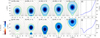 |
Fig. 1. Coronal flux rope eruptions caused by normal flux feeding. The top panels show the simulation results of flux ropes in the BPS configuration, which were adapted from Zhang et al. (2020). The bottom panels show the results for the HFT configuration, adapted from Zhang et al. (2021b). The black curves in panels (a)–(e) and (g)–(k) illustrate the temporal evolution of the magnetic field configuration, the green curves mark the boundary of the flux rope and that of the emerging fibril (panel (h)), and the distribution of the axial magnetic flux in the z−direction is shown in blue and red. Panels (f) and (l) show the evolutions of the height of the flux rope axis. The vertical dotted lines in panels (f) and (g) correspond to the times of panels (a)–(e) and panels (g)–(k), respectively. |
It is noteworthy that in all the previous simulations about flux feeding, the direction of the axial magnetic field within the rising fibril was the same as that within the preexisting flux rope, so that the total axial magnetic flux of the rope always accumulated after this type of flux feeding. Many observational studies demonstrated, however, that the chirality and helicity of newly emerging magnetic flux might be quite different from that of the magnetic system within the surrounding active region (e.g., Zhang 2001; Yang et al. 2009; Cheung & Isobe 2014; van Driel-Gesztelyi & Green 2015). This indicates that the axial magnetic field within chromospheric fibrils in the actual solar corona might not always be the same as that within the preexisting flux rope. In other words, flux feeding might also inject axial flux into the flux rope in the opposite direction, which is therefore referred to as inverse flux feeding in the remainder of this paper. For comparison, the flux feeding processes investigated in previous simulations are called normal flux feeding. Different from normal flux feeding, the total axial flux of the rope might not always accumulate after inverse flux feeding. It is still unclear how the flux rope system is affected by inverse flux feeding and whether inverse flux feeding is also able to cause solar eruptions. In this paper, we carried out 2.5-dimensional numerical simulations to investigate the evolution of coronal flux ropes associated with inverse flux feeding in the BPS and the HFT configurations, and we then compared our simulation results with those associated with normal flux feeding in previous studies to expand and improve the flux feeding mechanism of solar eruptions. The rest of this paper is arranged as follows: the numerical model used in our simulation is introduced in Sect. 2, the simulation results for the BPS and the HFT configurations are presented in Sects. 3.1 and 3.2, respectively, and the discussion and conclusion are given in Sect. 4.
2. Numerical model
2.1. Basic equations
In our 2.5-dimensional simulations, all the quantities satisfied ∂/∂z = 0, so that the magnetic field was written in the following form:
 (1)
(1)
where ψ is the magnetic flux function. With this form, the divergence-free condition of the magnetic field, ▿ ⋅ B = 0, is always satisfied. The MHD equations were then cast in the nondimensional form,
 (2)
(2)
 (3)
(3)
 (4)
(4)
 (5)
(5)
![Mathematical equation: $$ \begin{aligned} \nonumber&\frac{\partial T}{\partial t}-\frac{\eta (\gamma -1)}{\rho R}\left[(\vartriangle \psi )^2+|\triangledown \times (B_z\hat{\boldsymbol{z}})|^2 \right]\\&~~~+\boldsymbol{v}\cdot \triangledown T +(\gamma -1)T\triangledown \cdot \boldsymbol{v}=0, \end{aligned} $$](/articles/aa/full_html/2025/10/aa55545-25/aa55545-25-eq6.gif) (6)
(6)
where
 (7)
(7)
Here ρ, v, and T denote the density, velocity, and temperature, respectively; the subscripts x, y, z represent the x, y, and z components of the quantities; the polytropic index is γ = 5/3; g and η are the normalized gravity and the resistivity, respectively; β0 = 2μ0ρ0RT0L02/ψ02 = 0.1 is the characteristic ratio of the gas pressure to the magnetic pressure, where ρ0 = 3.34 × 10⁻¹³ kg m−3, T0 = 106 K, L0 = 107 m, and ψ0 = 3.73 × 10³ Wb m−1 are the characteristic values of the quantities. The equations introduced above were then solved by the multistep implicit scheme (Hu 1989; Hu et al. 2003) to simulate the evolution of the coronal magnetic system. The numerical domain was 0 < x < 200 Mm, 0 < y < 300 Mm; it was discretized into 400×600 uniform meshes. At the left side of the domain (x = 0), the symmetric boundary condition was used. Except during the flux feeding process (which will be introduced in Sect. 2.2), the lower boundary was always fixed; this implies that the lower boundary corresponds to the photosphere. At the other boundaries, increment equivalent extrapolation was used (e.g., Zhang et al. 2020),
Here, U represents the quantities in our simulation, including ρ, v, ψ, Bz, and T; the superscripts n and n + 1 indicate the quantities at the current and the next time steps, respectively, and the subscripts b and b − 1 indicate the quantities at the boundary and those at the location next to the boundary, respectively. The radiation and the heat conduction in the energy equation were neglected.
2.2. Simulating procedures
The initial states in our simulations for the BPS and HFT cases in our simulations were the same as those in Paper I and Paper II, respectively. The magnetic properties of a coronal magnetic flux rope can be characterized by the axial magnetic flux passing through the cross section of rope, Φz, and the annular magnetic flux of the rope per unit length along the z-direction, Φp. For the BPS initial state illustrated in Fig. 1a, Φz0B = 9.31 × 10¹⁹ Mx and Φp0B = 1.49 × 10¹⁰ Mx cm−1; for the HFT initial state in Fig. 1g, Φz0H = 4.37 × 10¹⁹ Mx and Φp0H = 1.19 × 10¹⁰ Mx cm−1. The simulating procedures in our simulations were also similar as those in Paper I and Paper II: Starting from the corresponding initial state, we let a small flux rope emerge from the lower base of the initial states, and it then interacted with the preexisting flux ropes, representing the scenario of flux feeding. In the rest of this paper, the preexisting large flux rope is called major rope for simplicity.
The emergence of the small rope is achieved by the following procedures: The emergence began at t = 0 and ended at t = τE (for the BPS cases in Paper I, τE = 30τA, where τA = 17.4 s; for the HFT cases in Paper II, τE = 60τA). During this period, the small rope emerged from right below the major rope. The small rope emerged at a constant speed vE = 2a/τE, where a = 5 Mm is the radius of the small rope. During the emergence, for instance, at time t1 (0 ≤ t1 ≤ τE), the emerged part of the small rope at the lower base was located within −xE ≤ x ≤ xE, where xE = (a2 − hE2)1/2, hE = a(2t1/τE − 1). By adjusting the quantities at the lower boundary (y = 0, −xE ≤ x ≤ xE), we achieved the emergence of the small rope,
 (8)
(8)
 (9)
(9)
 (10)
(10)
 (11)
(11)
 (12)
(12)
Here ψi(x, y = 0) is the magnetic flux function of the initial state at the lower boundary; ψi(x, y = 0) in Fig. 1a and g have been given in Paper I and Paper II, respectively. The parameter CE determines the intensity of flux feeding: the larger CE, the stronger the magnetic field strength within the small rope, so that more magnetic flux is injected into the major rope, as suggested by Paper I and Paper II. In the remainder of this paper, the given dimensionless values of CE here are in units of 0.373 × 10¹⁰ Mx cm−1. Anomalous resistivity was used in the simulations by Paper I and Paper II,
 (13)
(13)
Here, L0 = 107 m, v0 = 128.57 km s−1, and μ0 is the vacuum magnetic permeability. For the BPS cases in Paper I, ηm = 10−4 and jc = 2.37 × 10⁻⁴ A m−2, and for the HFT cases in Paper II, ηm = 9.95 × 10⁻² and jc = 4.45 × 10⁻⁴ A m−2.
In our simulations, the values of the corresponding parameters (a, τE, ηm, jc, ...) for the BPS and the HFT cases were the same as those in Paper I and Paper II, respectively, except that the axial component of the magnetic field within the emerging small rope was negative (Eq. (10)), so that the direction of Bz in the small rope was opposite to the major rope. In this way, we may explicitly compare the influence of the inverse flux feeding processes on coronal flux rope systems with that of the normal ones investigated by Paper I and Paper II.
3. Simulation results
3.1. BPS configuration
The simulation results of typical inverse flux feeding processes in the BPS configuration are illustrated in Fig. 2; the top row and the bottom row show the cases with CE = 1.85 and 1.90, respectively. After the onset of the inverse flux feeding process, the emerging small rope interacts and merges with the lower section of the major flux rope, which is similar as the process in Linton et al. (2001) and Linton (2006), for example. As a result, the negative axial magnetic flux within the small rope is injected into the major rope, as shown in red in Figs. 2a and f. The injected flux is then transported across the major rope (Figs. 2a–b and Figs. 2f–g), and the magnetic configuration of the resultant major rope after inverse flux feeding (Figs. 2b and g) is interesting: the injected negative axial flux does not completely cancel out with the preexisting positive axial flux within the central region of the major rope, but is eventually dispersed only within the outer section of the major rope, resulting in a double-layer configuration. It is noteworthy that the positive axial magnetic flux is concentrated in the central region of the major rope in the initial state (Fig. 1a). Since the negative axial flux injected by inverse flux feeding is primarily distributed in the outer section of the resultant major rope, the cancellation between the oppositely directed axial fluxes should be limited. The spatial separation of the preexisting positive and the injected negative axial fluxes leads to the formation of the double-layer configuration.
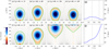 |
Fig. 2. Simulation results of the flux rope in the BPS configuration. Panels (a)–(d) illustrate the evolution of the magnetic configuration for the case with CE = 1.85, and panel (e) plots the evolution of the height of the rope axis. The vertical dotted lines correspond to the times of panels (a)–(d). Panels (f)–(l) show the results for the case with CE = 1.90. The meanings of the symbols and colors are the same as in Fig. 1. |
The subsequent evolutions of the major flux rope after flux feeding in the cases with CE = 1.85 and 1.90 are quite different. The major rope remains sticking to the photosphere in the case with CE = 1.85 (Figs. 2c–e), indicating that this is a noneruptive case. In the case with CE = 1.90, however, the major rope keeps rising after flux feeding, resulting in a full eruption of the major rope (Figs. 2h–j). The total axial current in the major rope during the onset of the eruption is about 7 × 10¹⁰ A, which is close to that during the eruption caused by normal flux feeding (Figs. 1a–f). This indicates that the strapping field strength is similar. It is interesting that the major rope remains in the double-layer configuration during its whole evolution, with the positive and negative axial flux separated from each other.
The resultant double-layer configuration of the major rope after inverse flux feeding might be explained by force-free flux rope model. For one-dimensional force-free flux tubes, Lundquist (1951) gave a flux rope model with the Lundquist solution,
 (14)
(14)
where r is the radial distance from the rope axis. An example of the radial distribution of the axial component of the magnetic field, Bz(r), predicted by the Lundquist solution is plotted in Fig. 3a (assuming B0 = 10 G and k = 100 Mm). The axial component of the magnetic field reverses direction at the zeros of Bz(r), which is usually regarded as undesirable feature for solar applications. In our simulations, however, this type of the Bz profile was found to exist within the flux rope: Fig. 3b plots the distribution of Bz along the gray dashed line in Fig. 2d; the Bz profile within the rope in our simulation is similar as that within the second zeropoint (marked by “B” in Fig. 3a) of Bz(r) in the Lundquist solution. Therefore, the Lundquist solution might explain the double-layer equilibrium state in our simulation, and our simulation results in turn indicate that axial magnetic field reversals might exist within solar magnetic flux ropes. We note that our simulation is not force-free and the flux rope in our simulation is not one-dimensional, so that the distribution of Bz in our simulation does not exactly follow that predicted by Lundquist solution.
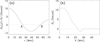 |
Fig. 3. Comparison of the radial distribution of Bz predicted by the model and that in our simulation results. Panel (a) shows the distribution of Bz predicted by the Lundquist solution, in which A and B mark the zeropoint. Panel (b) is the distribution of Bz along the dashed gray line in Fig. 2(d). |
To investigate the influence of inverse flux feeding on coronal flux ropes, we calculated the magnetic fluxes of the resultant major flux rope at t = 30τA and compared them with those of the initial BPS state, that is, Φz0B and Φp0B. The poloidal magnetic flux Φp remained unchanged after inverse flux feeding in both the cases with CE = 1.85 and 1.90, whereas the axial magnetic flux Φz decreased to 6.68 × 10¹⁹ Mx and 6.43 × 10¹⁹ Mx in the cases with CE = 1.85 and 1.90, respectively. We note that what we calculated above is the total signed axial magnetic flux of the rope. Because positive and negative axial fluxes are both distributed within the resultant major rope (Fig. 2b and g), we also calculated the total unsigned axial magnetic flux, |Φz|. For the initial BPS state, |Φz|0B = Φz0B = 9.31 × 10¹⁹ Mx; for the resultant rope after inverse flux feeding, |Φz| increases to 1.15×10²⁰ Mx and 1.17×10²⁰ Mx in the case with CE = 1.85 and 1.90, respectively. The total unsigned axial flux clearly accumulates after inverse flux feeding.
Following Paper I, we simulated many cases with different CE to investigate what initiates the eruption. The signed axial fluxes of the corresponding resultant major rope are plotted in Fig. 4a, and the unsigned axial fluxes in Fig. 4b. For the case with larger CE, that is, stronger intensity of inverse flux feeding, the total signed axial flux Φz of the resultant rope is lower, but the unsigned aixal flux |Φz| is higher, indicating that more negative flux is injected into the major rope. Moreover, |Φz| of the resultant rope in the eruptive cases (dots in Fig. 4b) tends to be higher than that in the noneruptive cases (small circles in Fig. 4b). We therefore infer that the total unsigned axial flux |Φz| rather than the signed flux Φz plays a decisive role in triggering the eruption of the flux rope. To confirm this, we further simulated many other cases, the initial states of which were changed to the resultant flux ropes in the noneruptive cases plotted in Fig. 4b. For simplicity, we call these cases second round of inverse flux feeding, and they are plotted in Fig. 4c. Those plotted in Fig. 4b are called first round of inverse flux feeding. The second rounds of flux feeding cases and their corresponding initial states are plotted by the same color, and are also connected by the dashed colored lines. Combining Figs. 4b and c, we suggest that the eruptive (dots) and the no-eruptive (small circles) cases are well separated, that is, there should be a critical value of the unsigned axial flux |Φz|cB of about 1.17 × 10²⁰ Mx, as marked by the horizontal dotted line in Figs. 4b–c. This value is very close to the critical Φz associated with normal flux feeding found by Paper I; since there is only positive magnetic flux within the resultant rope after normal flux feeding (Fig. 1), |Φz| always equals Φz in the simulation results in Paper I, indicating that the critical |Φz| associated with normal (Paper I) and inverse (this paper) flux feeding are very close. Therefore, we conclude that normal and inverse flux feeding processes are both able to cause coronal flux rope eruptions in BPS configurations. The onset of the eruption is not dominated by the total singed axial flux, but by the total unsigned axial flux |Φz|: The flux rope only erupts when its |Φz| surpasses the critical value |Φz|cB.
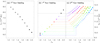 |
Fig. 4. Axial magnetic fluxes of the resultant major rope after inverse flux feeding with different CE. Φz and |Φz| of the resultant ropes after the first round of inverse flux feeding are plotted in panels (a) and (b), respectively, and panel (c) shows |Φz| of the resultant ropes after the second round of inverse flux feeding. The eruptive cases are plotted as dots, and the noneruptive cases are plotted as small circles. The correspondence between the cases in panel (c) and the corresponding new initial state is indicated by the dashed colored line. |
3.2. HFT configuration
Figure 5 illustrates the simulation results of typical inverse flux feeding processes in the HFT configuration; the top and bottom rows show the cases with CE = 2.10 and 2.15, respectively. After the inverse flux feeding process begins, the small rope emerges from the photosphere (Fig. 5a), pushing the arcades (marked by the green curves below the major rope in Fig. 1g) upward, which reconnect with the magnetic field of the major rope. The interaction and reconnection between the major rope and the arcades have been demonstrated in detail in Paper II. After all the arcades reconnect with the major rope, the small emerging rope itself interacts and merges with the major rope (Fig. 5b), during which negative axial magnetic flux carried by the small rope is injected into the major rope. As illustrated in Figs. 5c–5d, the injected flux is eventually distributed within the outer section of the major rope, which results in a double-layer configuration that is similar as that in the BPS cases (e.g., Fig. 2c). The simulation results demonstrate that the case with CE = 2.10 is noneruptive: The flux rope eventually falls down to the photosphere (Fig. 5d), so that the HFT configuration collapses. In the case with CE = 2.15, however, the resultant rope keeps rising after inverse flux feeding, so that this is an eruptive case. Following Paper II, we also calculated the magnetic fluxes of the resultant major rope. For the case with CE = 2.10, Φz = 5.78 × 10¹⁸ Mx, |Φz| = 7.05 × 10¹⁹ Mx, Φp = 1.12 × 10¹⁰ Mx cm−1, and for the case with CE = 2.15, Φz = 7.32 × 10¹⁷ Mx, |Φz| = 7.58 × 10¹⁹ Mx, Φp = 1.12 × 10¹⁰ Mx cm−1. Φz clearly decreases, but |Φz| accumulates after inverse flux feeding. Because larger CE implies a stronger intensity of the inverse flux feeding, more negative axial flux is injected, resulting in a higher |Φz| of the resultant rope. In both of these two cases, the poloidal flux of the major rope is reduced by about △Φp = 0.07 × 10¹⁰ Mx cm−1 after inverse flux feeding. As discussed by Paper II, the reduced poloidal flux is caused by the reconnection between the arcades below the rope (Fig. 1g) and the major rope, which peels off the outermost section of the major rope. The total axial current in the major rope during the onset of the eruption in the case with CE = 2.15 is about 7 × 10¹⁰ A, which is also close to that during the eruption caused by normal flux feeding (Figs. 1h–l).
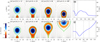 |
Fig. 5. Simulation results of the flux rope in the HFT configuration. The top and bottom panels show the results for the case with CE = 2.10 and CE = 2.15, respectively. The meanings of the symbols and colors are the same as in Fig. 1. |
We also further simulated many cases with different CE and discovered that the eruptive and noneruptive cases were also well separated. The cases with CE ≤ 2.10 (for the corresponding resultant major rope, |Φz|≤7.05 × 10¹⁹ Mx) are noneruptive, whereas the cases with CE≥ 2.11 (for the corresponding resultant major rope, |Φz|≥7.19 × 10¹⁹ Mx) are eruptive. This indicates that there is a critical unsigned axial flux of about 7.10 × 10¹⁹ Mx, which is almost the same as that was found by Paper II. Therefore, normal and inverse flux feeding processes are both able to cause the eruption of coronal flux ropes in the HFT configuration, provided that the critical |Φz| is reached after flux feeding. This conclusion is quite similar as that for the BPS cases.
4. Discussion and conclusion
In this paper, we investigated the influence of inverse flux feeding on coronal magnetic flux rope systems. During inverse flux feeding processes, newly emerging magnetic flux directly interacts with the preexisting coronal magnetic flux rope. As a result, the axial magnetic flux, whose direction is opposite to that within the preexisting major flux rope, is injected into the rope. The injected axial flux is distributed within the outer section of the major rope (Figs. 2 and 5), so that the total signed axial flux of the major rope decreases, but the total unsigned axial flux increases after inverse flux feeding. Our simulation results suggest that the onset of the eruption is associated with the total unsigned axial flux of the major rope. When the amount of the axial flux that is injected by inverse flux feeding is high enough for the unsigned axial flux of the major rope to exceed a critical value, the eruption of the coronal flux rope is initiated. As discussed in Sect. 3.1 and Sect. 3.2, although the signed axial fluxes after normal and inverse flux feeding are quite different, the values of the critical unsigned axial flux for inverse flux feeding are very close to those for normal flux feeding in both the BPS and the HFT cases. This indicates that not the signed, but the unsigned axial flux dominates the onset of the eruption, and the critical unsigned axial flux is almost the same, regardless of whether normal or inverse flux feeding occurs in the flux rope system. We therefore conclude that both normal and inverse flux feeding are efficient in causing coronal flux rope eruptions, provided that the critical unsigned axial flux of the rope is reached.
To further investigate the influence of flux feeding on the unsigned axial flux of coronal flux ropes, we simulated several additional cases, as shown in Fig. 6. Here we switched to use a new initial state, which was the resultant equilibrium state after the first round of inverse flux feeding in the BPS configuration with CE = 1.0 (corresponding to the small blue circle marked by the small arrow in Fig. 4b). Fig. 6a illustrates this new initial state, in which |Φz| = 9.75 × 10¹⁹ Mx. Negative axial flux is clearly distributed within the outer section of the major rope, which is different from the initial state of the simulation in Sect. 3.1 (Fig. 1a). Starting from this new initial state, we let a small flux rope containing positive axial flux emerge from the lower boundary, which is simply achieved by reversing the minus sign in Eq. (10). Figures 6b1–6b3 illustrate the corresponding simulation result with CE = 0.5: positive axial flux is injected into the major rope (Fig. 6b1 and the inset), and cancels out with the preexisting negative axial flux in the outer section of the major rope (Figs. 6b2–6b3). As a result, |Φz| decreases to 9.29 × 10¹⁹ Mx after this flux feeding process, and the rope does not erupt after flux feeding. In fact, the resultant rope in this case should be even further from the onset of the eruption than its initial state in Fig. 6a. This indicates that flux cancellation is possible during flux feeding when axial flux is present near the boundary of the flux rope, leading to a decrease rather than an accumulation of the total unsigned axial flux after flux feeding. It is noteworthy that this research focused on the influence of the flux feeding on the total magnetic flux of the flux rope and not on the detailed magnetic reconnection process of the oppositely directed axial flux, which can hardly be investigated under the translational invariance assumption in 2.5-dimensional simulations. For a stronger flux feeding process with CE = 1.5, not only the preexisting negative axial flux cancels out with the injected positive flux (Fig. 6c1), but additional positive axial flux is also injected into and then distributed within the outer section of the major rope (Figs. 6c2–c3). For this case with CE = 1.5, |Φz| increases to 1.15 × 10²⁰ Mx after flux feeding, but is still lower than the critical unsigned axial flux |Φz|cB ∼ 1.17 × 10²⁰ Mx, so that the major rope does not erupt (Fig. 6c4). For even stronger flux feeding process with CE = 2.0 (Figs. 6d1–6d4), |Φz| of the resultant rope is 1.22 × 10²⁰ Mx, which is higher than |Φz|cB, so that the major rope erupts eventually. These simulation results further confirm that the unsigned axial flux is very important, but it does not always accumulates after flux feeding. The properties of the flux feeding processes and the magnetic configuration of the preexisting coronal flux rope both influence the unsigned axial flux of the resultant rope after flux feeding.
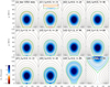 |
Fig. 6. Simulation results for the flux feeding processes in a flux rope system with double-layer configuration. Panel (a) shows the new initial state. Panels (b1)–(b3) show the evolution for the case with CE = 0.5, and the inset in panel (b1) corresponds to the region marked by the red box in panel (b). Panels (c1)–(c4) and panels (d1)–(d4) show the results for the cases with CE = 1.5 and CE = 2.0, respectively. The meanings of the symbols and colors are the same as in Fig. 1. |
An interesting phenomenon we found in our simulation results is that both positive and negative axial magnetic field can be distributed within a flux rope, as shown in Figs. 2 and 5, and the opposite axial magnetic field components within the flux rope also results in the coexistence of magnetic helicity with opposite signs within the rope. This type of double-layer configuration within the flux rope is the fundamental cause of the discrepancy between the signed and unsigned axial flux of the rope. Based on our simulation results, we inferred that reversals of the axial magnetic field component within the flux rope in the solar corona are possible. This implies that a flux rope might contain magnetic helicity of the opposite sign to that of the surrounding active region, and as a result, the magnetic helicity in the active region might even increase rather than decrease after the eruption of the flux rope. In fact, many previous studies have suggested that physical parameters related to magnetic helicity should play a critical role in the initiation of solar eruptions (e.g., Pariat et al. 2017; Zuccarello et al. 2018; Thalmann et al. 2019, 2020; Gupta et al. 2021). Therefore, in our future work, we plan to build upon the present study to explore helicity-related parameters as potential thresholds for the eruptions of flux ropes with complex internal structures. Moreover, interplanetary magnetic flux ropes might also exhibit this type of double-layer configuration, which might introduce new challenges for the modeling of magnetic clouds (e.g., Zhao et al. 2017). More observational and theoretical studies are still needed to further investigate the detailed magnetic topology inside coronal magnetic flux ropes and magnetic clouds, and the influence of the internal topological characteristics on the evolution of coronal flux ropes and magnetic clouds.
Acknowledgments
We appreciate Dr. Xiaolei Lei for his suggestion and advice. We also appreciate the anonymous referee for the valuable comments. This research is supported by the Strategic Priority Research Program of the Chinese Academy of Sciences (Grant No. XDB0560000), the National Natural Science Foundation of China (NSFC 42188101, 42174213, 11925302, 41804161), the Informatization Plan of Chinese Academy of Sciences (CAS-WX2022SF-0103), USTC Research Funds of the Double First-Class Initiative (YD2080002011), the open subject of Key Laboratory of Geospace Environment (GE2018-01), and the Innovation Program for Quantum Science and Technology (2021ZD0300302). We also acknowledge for the support from National Space Science Data Center, National Science "&" Technology Infrastructure of China (www.nssdc.ac.cn). Quanhao Zhang acknowledge for the support from Young Elite Scientist Sponsorship Program by the China Association for Science and Technology (CAST). Shangbin Yang acknowledge for the support from the National Key R&D Program of China No. 2022YFF0503800, 2021YFA1600500, 2022YFF0503001; the National Natural Science Foundation of China (grants No. 12250005, 12073040, 12273059, 11973056, 12003051, 11573037, 12073041, 11427901, 11572005, 11611530679 and 12473052); the Strategic Priority Research Program of the China Academy of Sciences (grants No. XDA15052200, XDB09040200, XDA15010700, XDB0560301, and XDA15320102); and by the Chinese Meridian Project (CMP).
References
- Antiochos, S. K., DeVore, C. R., & Klimchuk, J. A. 1999, ApJ, 510, 485 [Google Scholar]
- Archontis, V., & Hood, A. W. 2008, ApJ, 674, L113 [Google Scholar]
- Aulanier, G., Pariat, E., & Démoulin, P. 2005, A&A, 444, 961 [NASA ADS] [CrossRef] [EDP Sciences] [Google Scholar]
- Bi, Y., Jiang, Y., Yang, J., et al. 2016, Nat. Commun., 7, 13798 [Google Scholar]
- Chen, B., Yu, S., Reeves, K. K., & Gary, D. E. 2020, ApJ, 895, L50 [NASA ADS] [CrossRef] [Google Scholar]
- Chen, F., Rempel, M., & Fan, Y. 2023, ApJ, 950, L3 [NASA ADS] [CrossRef] [Google Scholar]
- Chen, P. F., & Shibata, K. 2000, ApJ, 545, 524 [Google Scholar]
- Cheng, X., Ding, M. D., Zhang, J., et al. 2014, ApJ, 789, 93 [Google Scholar]
- Cheung, M. C. M., & Isobe, H. 2014, Liv. Rev. Sol. Phys., 11, 3 [Google Scholar]
- Chintzoglou, G., Vourlidas, A., Savcheva, A., et al. 2017, ApJ, 843, 93 [Google Scholar]
- Chintzoglou, G., Zhang, J., Cheung, M. C. M., & Kazachenko, M. 2019, ApJ, 871, 67 [NASA ADS] [CrossRef] [Google Scholar]
- Démoulin, P., & Aulanier, G. 2010, ApJ, 718, 1388 [Google Scholar]
- Fan, Y. 2020, ApJ, 898, 34 [Google Scholar]
- Forbes, T. G., & Priest, E. R. 1995, ApJ, 446, 377 [NASA ADS] [CrossRef] [Google Scholar]
- Gibson, S. E., & Fan, Y. 2006, ApJ, 637, L65 [Google Scholar]
- Gopalswamy, N., Akiyama, S., Yashiro, S., & Xie, H. 2018, J. Atmosph. Solar-Terrest. Phys., 180, 35 [Google Scholar]
- Green, L. M., Török, T., Vršnak, B., Manchester, W., & Veronig, A. 2018, Space Sci. Rev., 214, 46 [Google Scholar]
- Guo, Y., Schmieder, B., Démoulin, P., et al. 2010, ApJ, 714, 343 [Google Scholar]
- Guo, J., Dumbović, M., Wimmer-Schweingruber, R. F., et al. 2018, Space Weather, 16, 1156 [NASA ADS] [CrossRef] [Google Scholar]
- Gupta, M., Thalmann, J. K., & Veronig, A. M. 2021, A&A, 653, A69 [NASA ADS] [CrossRef] [EDP Sciences] [Google Scholar]
- Hu, Y. Q. 1989, J. Comput. Phys., 84, 441 [NASA ADS] [CrossRef] [Google Scholar]
- Hu, Y. Q., Li, G. Q., & Xing, X. Y. 2003, J. Geophys. Res. (Space Phys.), 108, 1072 [Google Scholar]
- Inoue, S., Bamba, Y., & Kusano, K. 2018, J. Atmosph. Solar-Terrest. Phys., 180, 3 [Google Scholar]
- Jenkins, J. M., Long, D. M., van Driel-Gesztelyi, L., & Carlyle, J. 2018, Sol. Phys., 293, 7 [Google Scholar]
- Jiang, C., Duan, A., Zou, P., et al. 2023, MNRAS, 525, 5857 [NASA ADS] [CrossRef] [Google Scholar]
- Keppens, R., Guo, Y., Makwana, K., et al. 2019, Rev. Mod. Plasma Phys., 3, 14 [Google Scholar]
- Kliem, B., & Török, T. 2006, Phys. Rev. Lett., 96, 255002 [Google Scholar]
- Ledentsov, L. 2021, Sol. Phys., 296, 74 [NASA ADS] [CrossRef] [Google Scholar]
- Li, H., Liu, Y., Elmhamdi, A., & Kordi, A.-S. 2016a, ApJ, 830, 132 [Google Scholar]
- Li, T., Yang, K., Hou, Y., & Zhang, J. 2016b, ApJ, 830, 152 [CrossRef] [Google Scholar]
- Li, L., Song, H., Hou, Y., et al. 2025, ApJ, 979, 113 [Google Scholar]
- Li, X., Wang, Y., Guo, J., & Lyu, S. 2022, ApJ, 928, L6 [NASA ADS] [CrossRef] [Google Scholar]
- Li, X., Keppens, R., & Zhou, Y. 2023, ApJ, 947, L17 [NASA ADS] [CrossRef] [Google Scholar]
- Lin, J., Soon, W., & Baliunas, S. L. 2003, New Astron. Rev., 47, 53 [Google Scholar]
- Linton, M. G. 2006, J. Geophys. Res. (Space Phys.), 111, A12S09 [Google Scholar]
- Linton, M. G., Dahlburg, R. B., & Antiochos, S. K. 2001, ApJ, 553, 905 [NASA ADS] [CrossRef] [Google Scholar]
- Liu, R. 2020, Res. Astron. Astrophys., 20, 165 [Google Scholar]
- Longcope, D. W., & Forbes, T. G. 2014, Sol. Phys., 289, 2091 [Google Scholar]
- Lugaz, N., Farrugia, C. J., Winslow, R. M., et al. 2017, ApJ, 848, 75 [Google Scholar]
- Lundquist, S. 1951, Phys. Rev., 83, 307 [NASA ADS] [CrossRef] [Google Scholar]
- Mei, Z., Ye, J., Li, Y., et al. 2023, ApJ, 958, 15 [Google Scholar]
- Moore, R. L., Sterling, A. C., Hudson, H. S., & Lemen, J. R. 2001, ApJ, 552, 833 [Google Scholar]
- Owens, M. J. 2020, Sol. Phys., 295, 148 [Google Scholar]
- Pariat, E., Leake, J. E., Valori, G., et al. 2017, A&A, 601, A125 [CrossRef] [EDP Sciences] [Google Scholar]
- Patsourakos, S., Vourlidas, A., Török, T., et al. 2020, Space Sci. Rev., 216, 131 [Google Scholar]
- Savcheva, A. S., van Ballegooijen, A. A., & DeLuca, E. E. 2012, ApJ, 744, 78 [Google Scholar]
- Schwenn, R. 2006, Liv. Rev. Sol. Phys., 3, 2 [Google Scholar]
- Shibata, K., & Magara, T. 2011, Liv. Rev. Sol. Phys., 8, 6 [Google Scholar]
- Su, W., Wang, Y., Zhou, C., et al. 2021, ApJ, 914, 139 [Google Scholar]
- Su, W., Zhou, Z.-B., Wang, Y., et al. 2023, Phys. Rev. D, 108, 103030 [Google Scholar]
- Syntelis, P., Lee, E. J., Fairbairn, C. W., Archontis, V., & Hood, A. W. 2019, A&A, 630, A134 [EDP Sciences] [Google Scholar]
- Temmer, M. 2021, Liv. Rev. Sol. Phys., 18, 4 [NASA ADS] [CrossRef] [Google Scholar]
- Thalmann, J. K., Linan, L., Pariat, E., & Valori, G. 2019, ApJ, 880, L6 [Google Scholar]
- Thalmann, J. K., Sun, X., Moraitis, K., & Gupta, M. 2020, A&A, 643, A153 [EDP Sciences] [Google Scholar]
- Titov, V. S., Priest, E. R., & Demoulin, P. 1993, A&A, 276, 564 [NASA ADS] [Google Scholar]
- Titov, V. S., Galsgaard, K., & Neukirch, T. 2003, ApJ, 582, 1172 [Google Scholar]
- Toriumi, S. 2014, PASJ, 66, S6 [NASA ADS] [CrossRef] [Google Scholar]
- Török, T., & Kliem, B. 2003, A&A, 406, 1043 [NASA ADS] [CrossRef] [EDP Sciences] [Google Scholar]
- Török, T., Linton, M. G., Leake, J. E., et al. 2024, ApJ, 962, 149 [CrossRef] [Google Scholar]
- Švestka, Z. 2001, Space Sci. Rev., 95, 135 [Google Scholar]
- van Driel-Gesztelyi, L., & Green, L. M. 2015, Liv. Rev. Sol. Phys., 12, 1 [Google Scholar]
- Van Tend, W., & Kuperus, M. 1978, Sol. Phys., 59, 115 [Google Scholar]
- Vemareddy, P., Cheng, X., & Ravindra, B. 2016, ApJ, 829, 24 [NASA ADS] [CrossRef] [Google Scholar]
- Veronig, A. M., Podladchikova, T., Dissauer, K., et al. 2018, ApJ, 868, 107 [NASA ADS] [CrossRef] [Google Scholar]
- Vršnak, B., Sudar, D., & Ruždjak, D. 2005, A&A, 435, 1149 [NASA ADS] [CrossRef] [EDP Sciences] [Google Scholar]
- Yan, X. L., Wang, J. C., Pan, G. M., et al. 2018, ApJ, 856, 79 [NASA ADS] [CrossRef] [Google Scholar]
- Yang, S., Zhang, H., & Büchner, J. 2009, A&A, 502, 333 [NASA ADS] [CrossRef] [EDP Sciences] [Google Scholar]
- Ye, J., Raymond, J. C., Mei, Z., et al. 2023, ApJ, 955, 88 [NASA ADS] [CrossRef] [Google Scholar]
- Zhang, H. 2001, MNRAS, 326, 57 [Google Scholar]
- Zhang, J., Dere, K. P., Howard, R. A., Kundu, M. R., & White, S. M. 2001, ApJ, 559, 452 [Google Scholar]
- Zhang, Q., Liu, R., Wang, Y., et al. 2014, ApJ, 789, 133 [Google Scholar]
- Zhang, Q., Wang, Y., Hu, Y., & Liu, R. 2016, ApJ, 825, 109 [Google Scholar]
- Zhang, Q., Wang, Y., Liu, R., et al. 2020, ApJ, 898, L12 [Google Scholar]
- Zhang, Q., Liu, R., Wang, Y., Li, X., & Lyu, S. 2021a, ApJ, 921, 172 [Google Scholar]
- Zhang, Q., Liu, R., Wang, Y., et al. 2021b, A&A, 647, A171 [NASA ADS] [CrossRef] [EDP Sciences] [Google Scholar]
- Zhang, Q. M., Cheng, J. X., Feng, L., et al. 2019, ApJ, 883, 124 [Google Scholar]
- Zhao, A., Wang, Y., Liu, J., et al. 2017, ApJ, 845, 109 [Google Scholar]
- Zuccarello, F. P., Pariat, E., Valori, G., & Linan, L. 2018, ApJ, 863, 41 [Google Scholar]
All Figures
|
Fig. 1. Coronal flux rope eruptions caused by normal flux feeding. The top panels show the simulation results of flux ropes in the BPS configuration, which were adapted from Zhang et al. (2020). The bottom panels show the results for the HFT configuration, adapted from Zhang et al. (2021b). The black curves in panels (a)–(e) and (g)–(k) illustrate the temporal evolution of the magnetic field configuration, the green curves mark the boundary of the flux rope and that of the emerging fibril (panel (h)), and the distribution of the axial magnetic flux in the z−direction is shown in blue and red. Panels (f) and (l) show the evolutions of the height of the flux rope axis. The vertical dotted lines in panels (f) and (g) correspond to the times of panels (a)–(e) and panels (g)–(k), respectively. |
| In the text | |
|
Fig. 2. Simulation results of the flux rope in the BPS configuration. Panels (a)–(d) illustrate the evolution of the magnetic configuration for the case with CE = 1.85, and panel (e) plots the evolution of the height of the rope axis. The vertical dotted lines correspond to the times of panels (a)–(d). Panels (f)–(l) show the results for the case with CE = 1.90. The meanings of the symbols and colors are the same as in Fig. 1. |
| In the text | |
|
Fig. 3. Comparison of the radial distribution of Bz predicted by the model and that in our simulation results. Panel (a) shows the distribution of Bz predicted by the Lundquist solution, in which A and B mark the zeropoint. Panel (b) is the distribution of Bz along the dashed gray line in Fig. 2(d). |
| In the text | |
|
Fig. 4. Axial magnetic fluxes of the resultant major rope after inverse flux feeding with different CE. Φz and |Φz| of the resultant ropes after the first round of inverse flux feeding are plotted in panels (a) and (b), respectively, and panel (c) shows |Φz| of the resultant ropes after the second round of inverse flux feeding. The eruptive cases are plotted as dots, and the noneruptive cases are plotted as small circles. The correspondence between the cases in panel (c) and the corresponding new initial state is indicated by the dashed colored line. |
| In the text | |
|
Fig. 5. Simulation results of the flux rope in the HFT configuration. The top and bottom panels show the results for the case with CE = 2.10 and CE = 2.15, respectively. The meanings of the symbols and colors are the same as in Fig. 1. |
| In the text | |
|
Fig. 6. Simulation results for the flux feeding processes in a flux rope system with double-layer configuration. Panel (a) shows the new initial state. Panels (b1)–(b3) show the evolution for the case with CE = 0.5, and the inset in panel (b1) corresponds to the region marked by the red box in panel (b). Panels (c1)–(c4) and panels (d1)–(d4) show the results for the cases with CE = 1.5 and CE = 2.0, respectively. The meanings of the symbols and colors are the same as in Fig. 1. |
| In the text | |
Current usage metrics show cumulative count of Article Views (full-text article views including HTML views, PDF and ePub downloads, according to the available data) and Abstracts Views on Vision4Press platform.
Data correspond to usage on the plateform after 2015. The current usage metrics is available 48-96 hours after online publication and is updated daily on week days.
Initial download of the metrics may take a while.