| Issue |
A&A
Volume 702, October 2025
|
|
|---|---|---|
| Article Number | A229 | |
| Number of page(s) | 18 | |
| Section | Extragalactic astronomy | |
| DOI | https://doi.org/10.1051/0004-6361/202555603 | |
| Published online | 22 October 2025 | |
GalIMF–E-MILES library: Impact of an environment-dependent initial mass function on stellar population spectra
1
Instituto de Astrofísica de Canarias (IAC), E-38200 La Laguna, Tenerife, Spain
2
Departamento de Astrofísica, Universidad de La Laguna, E-38205 Tenerife, Spain
3
Department of Physics, Institute for Advanced Studies in Basic Sciences (IASBS), 11365-9161 Zanjan, Iran
4
Department of Theoretical Physics and Astrophysics, Faculty of Science, Masaryk University, Kotlářská 2, Brno 611 37, Czech Republic
5
School of Astronomy and Space Science, Nanjing University, Nanjing, 210000, China
6
Key Laboratory of Modern Astronomy and Astrophysics, Nanjing University, Ministry of Education, Nanjing 210093, China
7
Helmholtz-Institut für Strahlen-und Kernphysik (HISKP), Universität Bonn, Nussallee 14-16, D-53115 Bonn, Germany
8
Charles University, Faculty of Mathematics and Physics, Astronomical Institute, V Holešovickách 2, CZ-18000 Prague, Czech Republic
⋆ Corresponding author: This email address is being protected from spambots. You need JavaScript enabled to view it.
Received:
20
May
2025
Accepted:
27
August
2025
Abstract
We present, for the first time, model spectra of single-age, single-metallicity stellar populations computed with the E-MILES evolutionary synthesis code incorporating an environment-dependent, variable galaxy-wide initial mass function (gwIMF). This gwIMF, calculated using the GalIMF code, is rooted in the integrated galactic initial mass function (IGIMF) theory, which predicts IMF variations as a function of the star formation rate and the metallicity. By coupling these two codes, we generated a comprehensive library of single-burst stellar population spectra uniquely sensitive to gwIMF variations. Through detailed comparisons with the canonical Milky-Way IMF, we reveal how both the spectral energy distributions and key stellar absorption features systematically evolve with age under different IMF conditions. Our results uncover clear spectral signatures tied to IMF variability, emphasising the critical role of star formation and chemical enrichment histories in shaping the integrated light observed in galaxies. Based on our work, specific absorption spectral indices emerge as powerful diagnostics, and they open new pathways to empirically test IMF variations and refine models of galaxy formation and evolution. All synthetic spectra generated in this study are publicly available and constitute a valuable resource for future observational and theoretical investigations.
Key words: galaxies: evolution / galaxies: formation / galaxies: luminosity function / mass function / galaxies: stellar content
© The Authors 2025
 Open Access article, published by EDP Sciences, under the terms of the Creative Commons Attribution License (https://creativecommons.org/licenses/by/4.0), which permits unrestricted use, distribution, and reproduction in any medium, provided the original work is properly cited.
This article is published in open access under the Subscribe to Open model. This email address is being protected from spambots. You need JavaScript enabled to view it. to support open access publication.
1. Introduction
The shape of the initial mass function (IMF) is a key ingredient of stellar population synthesis (SPS), as evidenced by the seminal studies of Tinsley (1968) and Tinsley & Gunn (1976). When a stellar cluster or galaxy cannot be resolved, the observed light represents the combined total light of its constituent stars. By integrating theoretical or empirical stellar spectra corresponding to stars with varying ages and masses, it is possible to make predictions of stellar populations with varying properties. The prediction that provides the best fit to the observation of distant objects is considered to be the most accurate description of their stellar populations. A comprehensive description of the SPS approach, its advantages, and its limitations can be found in Leitherer & Ekström (2011), Conroy (2013), Eldridge et al. (2017) and Stanway (2020), for example.
More recent stellar population studies of galaxies consider that single burst (single-age and single-metallicity stellar populations) or, simply, single stellar populations (SSPs) are the building blocks of more complex stellar populations. SSPs are composed of stars formed simultaneously from the same initial gas and dust composition, for which we adopt a specific IMF. SSPs can also be used as simplified models for understanding the main properties of a galaxy.
Typically, SSP models are constructed by assuming an age and chemical composition (metallicity) for the stellar population. The approach requires stellar evolution models to predict how stars of different masses and compositions evolve over time in terms of luminosity and temperature. By adopting an IMF, which determines the mass distribution of stars, the integrated spectrum of all stars in the SSP can be computed. As a result, we obtain a synthetic spectrum that represents the collective light emitted by the entire population, as well as a variety of photometric properties. The models used in the current work are based on the SPS codes of Vazdekis et al. (1996) and Vazdekis et al. (2010).
One of the purposes of SPS is to model observed galaxy spectra, which provides a wealth of information regarding the fundamental properties of a set of galaxies. The comparison of modelled and observed galaxy spectra allows relevant parameters to be derived, such as the star formation history (SFH), the stellar metallicity, the stellar abundance pattern, the IMF, and the total mass of stars. Moreover, the properties derived from galaxy spectra have formed the basis of our current understanding of galaxy formation and evolution (Conroy 2013).
As explained above, the shape of the IMF is essential for characterising a stellar population and its associated spectrum. Since first being introduced by Salpeter (1955), the IMF has been used to describe the initial distribution of star masses. The number of stars that form within certain mass ranges has traditionally been described by a power law function: ξ(m)=dN/dm ∝ m−α. Subsequently, the IMF has been revised by several authors, such as Schmidt (1959), Miller & Scalo (1979), Scalo (1986), Kroupa et al. (1993), Vazdekis et al. (1996), and Chabrier (2003). Among them, Kroupa (2001) proposed a universal IMF consistent with constraints from local star-count data, keeping α = 2.3 above half a solar mass but introducing α = 1.3 between 0.08 − 0.5 M⊙ and α = 0.3 below 0.08 M⊙. This canonical and invariant IMF is established by the observation of Galactic field stars and open star clusters with a large uncertainty on the shape of the IMF (Kroupa 2001, 2002). There is a tendency to assume a universal IMF, and it is often driven by established analysis pipelines and models. While this approach has provided a useful baseline, it can lead to incomplete interpretations if variations with mass range, redshift, spatial scale, or environmental conditions are not considered. To robustly test the universality or variability of the IMF, it is important to explicitly account for these potential dependencies rather than assume invariance by default.
Recent observations challenge the invariant IMF. For example, stars formed in vastly different environments (different gas density or metallicity) have been shown to have systematically different IMFs (Vazdekis et al. 2003; Lee et al. 2009; van Dokkum & Conroy 2010; Gunawardhana et al. 2011; Marks et al. 2012; Zhang et al. 2018; Zhou et al. 2019; Smith 2020; Martín-Navarro et al. 2021). There is evidence of IMF variation on small scales within a galaxy (i.e. individual star forming regions, Martín-Navarro et al. 2015; Van Dokkum et al. 2017; Schneider et al. 2018; La Barbera et al. 2019, 2021), and it has been deduced to vary with galaxy mass (e.g. Ferreras et al. 2013; La Barbera et al. 2013). Even for the Milky Way, environment-dependent IMF variations have begun to be detected with the newest generation of telescopes (Li et al. 2023). Additionally, the IMF has been examined to change over cosmic time (Vazdekis et al. 1996; Weidner et al. 2013). All of these issues need to be consistently explained by a unified IMF theory. In this context, we delve into the complexities of SSP research, emphasising the importance of considering varying IMFs, instead of a universal one.
A new theoretical framework based on empirical relations allows for systematic variations of the IMF with the star formation rate1 (SFR) of a galaxy, that is, the integrated galactic IMF (IGIMF) (Kroupa & Weidner 2003; Weidner & Kroupa 2005; Kroupa et al. 2013). The IGIMF empirically accounts for the varying physical and environmental conditions within a galaxy. It considers that the IMF might vary in regions with different metallicities, densities, or other factors. Instead of a single global IMF, it provides a range of molecular-cloud-scale IMFs. Importantly, the IGIMF links local IMFs to derive a global galaxy-wide IMF (gwIMF) (Kroupa & Weidner 2003). In scenarios where the IMF is not universal, it becomes essential to distinguish between the IMF defined on local versus global scales. The stellar IMF (sIMF) describes the distribution of stellar masses formed within an individual embedded cluster, typically on sub-parsec scales within a molecular cloud core. The gwIMF, by contrast, captures the integrated outcome of all sIMFs within a galaxy at a given time. For an SSP, the gwIMF represents the IMF across the entire star-forming environment of a galaxy within a single time step, corresponding to well-defined average conditions–specifically, the metallicity and SFR of the galaxy at that epoch (e.g. see Jeřábková et al. 2018).
Notably, SSPs may be used in both gwIMF and composite IMF (cIMF) contexts, depending on the scale and scope of the modelled or observed population. When interpreting results of individual SSPs, especially in the context of synthetic population modelling and observational diagnostics, the generic term IMF is often used regardless of whether the underlying IMF represents a local (sIMF-like) or global (gwIMF-like) configuration. This means that ensuring clear terminology is particularly important when connecting data interpretation to physical assumptions.
The previously described SSP-based gwIMF belongs to a galaxy ‘instant’. It must be distinguished from the time-integrated gwIMF used in SPS modelling. In the SPS context, the gwIMF is a global function describing the cumulative stellar mass distribution formed over the lifetime of the galaxy. It is typically derived by averaging the variable sIMF across the evolving conditions of star formation in a galaxy, weighted by the frequency and intensity of those conditions. The resulting time-integrated gwIMF accounts for all star-forming regions and epochs and is normalised to the total stellar mass of the galaxy. It thus explains the observed systematic variations in IMF-sensitive observables across different galaxies, which appear to correlate with galaxy-wide SFRs and metallicities (Kroupa et al. 2013).
The IGIMF theory has solved several previously outstanding extragalactic problems. For instance, this theory has provided an explanation of the UV extended galactic discs (Pflamm-Altenburg & Kroupa 2008) and naturally accounts for the time-scale problem for building up a sufficiently large stellar population in dwarf galaxies given their low SFRs (Pflamm-Altenburg & Kroupa 2009). The theory predicts that dwarf galaxies must show a deficit of Hα emission relative to UV emission (see Pflamm-Altenburg et al. 2007 and Pflamm-Altenburg et al. 2009). This was verified to be the case by Lee et al. (2009). A recent implementation of the IGIMF framework in SPS models has been presented by Zonoozi et al. (2025), who developed the SPS-VarIMF code to compute galaxy spectra, colours, and mass-to-light ratios for varying gwIMFs as a function of SFR and metallicity. Their results show that galaxy-wide photometric properties, such as UV-optical colours and mass-to-light ratios, are significantly affected by the choice of IMF. Furthermore, the implementation of the IGIMF theory in chemical evolution models leads to a better agreement with the observations (Gargiulo et al. 2015; Fontanot et al. 2016; Romano et al. 2017; Palla et al. 2020; Yan et al. 2020, 2021; Mucciarelli et al. 2021).
In this work, GalIMF serves as the computational application that calculates galaxy-property-dependent gwIMFs, according to the IGIMF theory (Yan et al. 2017; Jeřábková et al. 2018; Yan et al. 2020). This python3 module computes an environment-dependent IMF function by integrating over a whole galaxy, parametrised by metallicity and SFR2. While the metallicity shapes up the stellar mass distribution for the smallest stars (M-dwarfs), the IMF of the massive stars is more sensitive to the core density of the star-forming molecular clouds (Marks et al. 2012), which correlates with the galaxy-wide SFR.
Within this framework, there is a clear dependence of the SSPs (and their resulting spectra) on the input IMF, although SPS codes commonly assume a canonical invariant IMF as a default or other ad hoc invariant IMF formulations (Bruzual & Charlot 2003; Conroy et al. 2009; Leitherer et al. 1999; Vazdekis et al. 2010). Among them, E-MILES is a widely applied SPS code that relies on spectra of SSPs, and it is based on empirical stellar spectral libraries such as MILES (Vazdekis et al. 2010, 2016, 2020). Moreover, the E-MILES code is continuously updated (e.g. Vazdekis et al. 2020).
In this study, we present, for the first time, the IGIMF theory applied in the E-MILES SPS code in order to provide empirical spectra of SSPs. This is performed by introducing the python3 module GalIMF into the E-MILES modelling scheme. The GalIMF python module returns gwIMFs (not time integrated), which depend on the SFR and metallicity of the stellar population. The resulting stellar mass distribution (i.e. the IMF) will be used by E-MILES software to integrate star spectra along an isochrone, which takes into account the evolutionary status of the stars. In this way, it calculates synthetic spectra corresponding to SSPs with varying ages and metallicity. The coupling of GalIMF and EMILES codes leads to environment-dependant SSP spectra that are to be confronted with observed galaxy spectra in order to shed further light on their formation and evolution. The newly computed spectra open an unexplored path for studying how the IGIMF theory affects stellar population spectra. This is done by analysing the main differences in the flux and the sensitivity of key line-strength indices. Those are measured in the resulting spectra with respect to the ones predicted with a standard canonical IMF. We also discuss whether such differences can be detected in real galaxy spectra.
This work is organised as follows. In Sect. 2 we explain the methodology of the approach, the modelling of the gwIMF according to GalIMF, the characteristics of the E-MILES models, the connection between both codes, and the subsequent new gwIMF-depending spectral library. In Sect. 3 we present the results of the spectra and a set of derived indices, comparing the environment-dependent gwIMF with the canonical Milky-Way IMF. In Sect. 4 we discuss some of our findings and address further potential applications. In Sect. 5 we state the conclusions. Lastly, in Appendix A we present an extra set of index-results that might be of interest.
2. Modelling approach
The implementation of the GalIMF module in the E-MILES code enables the first SSP spectral library to be obtained based on the IGIMF theory and empirical stellar spectra. In this section, we briefly describe the E-MILES and GalIMF codes as well as their coupling.
2.1. E-MILES models
The E-MILES evolutionary synthesis code provides SSP model spectra3 spanning a wide range of ages, metallicities (including models with varying elemental abundance ratios), and a suite of IMF shapes and slopes (Vazdekis et al. 2010, 2016, 2020). The E-MILES SSP spectra cover the wavelength range from 1680 Å to 50 000 Å at moderately high spectral resolution. It is important to note that the nominal resolution is not constant across all wavelengths, as it is determined by the resolution of the empirical stellar libraries used to construct the models in each spectral window (see Vazdekis et al. 2016, for details). For the wavelengths of the current work (3540–7410 Å) the resolution is determined by a constant FWHM = 2.51 Å. In terms of the velocity dispersion, the resolution is given by σ ≈ 90 km s−1 at 3540 Å, σ ≈ 60 km s−1 in the middle of the range and σ ≈ 45 km s−1 at 7410 Å. This resolution is compatible with, or slightly above, the resolution typically allowed by the internal dynamics of most massive galaxies, as characterised by their velocity dispersion broadening.
Its main ingredients include the theoretical isochrones of Girardi et al. (2000), referred to as Padova00, and Pietrinferni et al. (2004), referred to as BaSTI. These isochrones describe the evolution of stars of different initial masses over time, which is reflected in their luminosity and temperature. The youngest isochrones included in this work, with ages of 63 Myr, contain stellar masses up to ≈7 M⊙, based on the Padova00 evolutionary tracks. We have also computed models for even younger stellar populations, although these are not presented in the current version. A detailed comparison of these two sets of isochrones can be found in Cassisi et al. (2004), Pietrinferni et al. (2004) and Vazdekis et al. (2015). These isochrones are converted to the observational plane following extensive photometric stellar libraries (Alonso-Herrero et al. 1996; Alonso et al. 1999). The stellar population models based on the Padova00 isochrones cover ages from 0.063 to 17.8 Gyr and seven metallicities: [M/H] (Z)= − 2.32 (0.0001), −1.71 (0.0004), −1.31 (0.001), −0.71 (0.004), −0.40 (0.008), 0.00 (0.019) and 0.22 (0.03). Here, the [M/H] (Z)=0.00 (0.019) represents the solar value, defined using the metal mixture from Grevesse & Noels (1993). The models based on the BaSTI isochrones cover ages from 0.03 to 14 Gyr and 12 metallicities: [M/H] (Z)= − 2.27 (0.0001), −1.79 (0.0003), −1.49 (0.0006), −1.26 (0.001), −0.96 (0.002), −0.66 (0.004), −0.35 (0.008), −0.25 (0.010), 0.06 (0.0198), 0.15 (0.024), 0.26 (0.030) and 0.40 (0.040). Younger SSP models, with ages < 63 Myr, have already been computed (Vazdekis et al. 2016), but are not yet implemented in the GalIMF–E-MILES library.
E-MILES employs empirical, flux-calibrated, single burst stellar spectral libraries, namely NGSL (Koekemoer et al. 2006; Gregg et al. 2006), MILES (Sánchez-Blázquez et al. 2006), Indo-US (Valdes et al. 2004), CaT (Cenarro et al. 2001), and IRTF (Cushing et al. 2005; Rayner et al. 2009), which together enable the computation of stellar population spectra across different spectral windows. We emphasise that the stellar spectra feeding the E-MILES synthesis code are purely empirical, meaning that each spectrum corresponds to an actual observed star rather than a theoretical model. Finally, the spectra computed in the different wavelength ranges are seamlessly joined to create a single, extended spectrum for each SSP.
These models are computed for different IMF shapes and slopes, which include the standard multipart power-law IMFs of Kroupa (2001), the log-normal IMF of Chabrier (2001), and the single and broken power-law IMFs described in Vazdekis et al. (1996), commonly regarded as unimodal and bimodal, respectively, and both with custom logarithmic slopes. We note that the single power-law IMF with slope 1.3 matches the IMF of Salpeter (1955). In this work, we expand the predictions of E-MILES by implementing gwIMFs obtained with the IGIMF theory.
Using E-MILES for computing the spectrum of a stellar population involves several steps. Briefly, for a given age and metallicity, the code integrates the star spectra along the selected isochrone. It does so by following the relative number of alive stars per mass bin that contributes to the total light of the stellar population. For each mass bin and spectral range, a stellar spectrum is computed following a local interpolation scheme. Such interpolation weights the closest stars available in every empirical stellar library according to their stellar atmospheric parameters, namely temperature, gravity, and metallicity. Finally, the resulting SSP spectra are combined to obtain the spectrum covering the whole wavelength range. For a more detailed description of the method, we refer the reader to Vazdekis et al. (2010) and Vazdekis et al. (2016).
For this work, we adopt the Padova00 isochrones, as in the solar metallicity case ([M/H] = 0) both the canonical IMF and the gwIMF (log10(SFR) = 0) exhibit the closest agreement4. Throughout this paper, we refer to the SFR, commonly denoted as ‘ψ(t)’ in the literature, simply as ‘SFR’.
To simplify the analysis, we restrict our study to the optical wavelength range of the MILES stellar library, covering from 3540 Å to 7410 Å. The SFR values quoted in this work are expressed in units of M⊙ yr−1.
2.2. The variable IMF theory – IGIMF
As addressed with several references in the introduction, a significant body of evidence points to the fact that the stellar IMF (sIMF) is not universal. These findings suggest that the sIMF changes with the environmental conditions in which stars are born. The IGIMF theory tackles this IMF variability by, in a nutshell, adopting an empirical environment-dependent IMF for embedded star clusters, and compounding the galactic stellar population from these star formation building blocks. This means, all the embedded star clusters formed within a short time interval (Kroupa & Weidner 2003; Weidner & Kroupa 2005; Kroupa et al. 2013, 2024). The resulting gwIMF depends on the metallicity and galaxy-wide SFR (Jeřábková et al. 2018), and therefore, on the chemical enrichment history and the SFH of a galaxy (Yan et al. 2019). In the IGIMF framework, the SFR is defined as the total stellar mass formed across the entire galaxy per unit time. Specifically, it is treated as a mean value over a characteristic time interval of 10 Myr, which reflects the typical duration of a star formation epoch. This timescale is motivated by the lifetimes of molecular clouds and the rapid dissolution of embedded clusters. The total number and mass distribution of star clusters formed within this period are regulated by the global SFR, which in turn determines the shape of the gwIMF through integration over all contributing clusters.
In this work, we follow the IGIMF formulation for intermediate and massive stars of Yan et al. (2017), assuming that the IMF slope for massive stars correlates with the mass (and less significantly on the metallicity) of an embedded star cluster (Marks et al. 2012), resulting in a good reproduction of the gwIMF–SFR relation observed in Lee et al. (2009), Gunawardhana et al. (2011) and Zhang et al. (2018). For the low-mass stars, we follow Equation (9) from Yan et al. (2020) where the IMF power-law index linearly correlates with the logarithm of the stellar metal mass fraction, in agreement with the observation of early-type galaxies (ETGs) near and far (Geha et al. 2013; Martín-Navarro et al. 2019; Lonoce et al. 2023; Yan et al. 2024). That is, the IGIMF theory adopts empirically motivated assumptions and returns a gwIMF, predicting how many more massive stars should form in a starburst galaxy and when a galaxy would stop forming any massive stars (Yan et al. 2017, their figure 7). The exact assumptions may be adjusted in the future given better constraints on the environmental dependency of the IMF. We adopt the GalIMF5 code version 1.1.10 for the calculation in this work.
It is worth mentioning that we explored systematic variations of the IMF that are empirically motivated. These variations are treated as deterministic inputs to our models and reflect changes in the underlying distribution function of stellar masses as a function of physical conditions such as the SFR and metallicity. However, in real systems, additional layers of uncertainty exist. For instance, Hennebelle & Grudić (2024) discuss how assumptions about IMF slopes are themselves subject to uncertainties, which can propagate into SSP predictions and become particularly relevant when comparing to high-quality observations. Another important aspect is how the IMF is sampled. In this study, we use optimal sampling (Yan et al. 2017), which ensures that the most massive star is physically consistent with the total stellar mass of the population. This deterministic approach avoids Poisson noise and is particularly useful when generating SSPs, where the aim is to isolate the effects of systematic IMF variation. Nonetheless, stochastic sampling effects can play a significant role, whether intrinsic to star formation or due to the limited number of stars observed, especially in low-mass or semi-resolved systems. These effects have been explored, for example, by Yan et al. (2023) and Byrne et al. (2025), along with the complementary work of Martín-Navarro & Vazdekis (2024), which highlights the growing importance of resolving these phenomena in practice. Future studies could therefore include both systematic IMF variation and stochastic sampling effects to better understand the resulting impact on observable quantities, and to quantify the extent to which observational scatter may reflect intrinsic versus extrinsic sources of stochasticity.
As an example of the GalIMF results, in Fig. 1 we display the calculated gwIMF for galaxy-wide SSPs formed in a δt = 10 Myr star formation epoch, with different metallicity and galactic SFRs. We display the combination of SFR such as log10(SFR) = −2, 0 and 2, with metallicities of [M/H] = −0.4, 0 and 0.22. We would like to emphasise that only stars with masses lower than the mass of the most massive surviving star will contribute to the galaxy-wide spectra, as indicated by the horizontal black arrows. For a better inspection, in Fig. 2 we represent these masses against the age of the population. Notice that the upper limit for the star mass in the canonical IMF is 150 M⊙, while in gwIMF, the maximum mass increases with the SFR value and depends on the embedded cluster mass, but never exceeds the 150 M⊙ threshold. Stars more massive than 150 M⊙ have been observed, but likely form through rare merger events of massive binary systems (Banerjee et al. 2012).
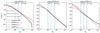 |
Fig. 1. Collection of IMFs (normalised to have the same mass). Columns correspond to log10(SFR) = −2, 0 and 2. Each panel shows the number of stars per mass interval: canonical IMF in red and gwIMF in a gradient of greys for each metallicity ([M/H] = −0.4, 0, and 0.22), from lightest to darkest. The vertical blue lines represent the mass of the most massive surviving star when the age of the population is 10, 1, and 0.1 Gyr, corresponding to ≈1.1, 2.3 and 5.4 M⊙ in each case (assuming solar metallicity). We note that only stars with masses lower than the mass of the most massive surviving star will contribute to the spectra, as the horizontal arrows of the first panel show. The normalisation is performed as explained in Sect. 2.4. |
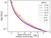 |
Fig. 2. Masses of the most massive surviving stars according to the age of the population. We show all the Padova00 metallicities, marking with a blue cross the cases of 10, 1, and 0.1 Gyr (correspondingly ≈1.1, 2.3 and 5.4 M⊙) for the solar metallicity, as in Fig. 1. |
2.3. E-MILES–GalIMF connection and SSP spectral library
In this work, we present for the first time the combination of GalIMF and E-MILES codes. The connection of both codes simultaneously provides the gwIMF and the spectrum of its associated SSP with a particular galactic SFR, stellar metallicity, and age.
On the one hand, the E-MILES code requires a metallicity, an age, and an IMF function as basic inputs for calculating the desired SSP model. On the other hand, the GalIMF code requires an SFR and a metallicity, returning the gwIMF (not time integrated). This gwIMF is saved and provided to the E-MILES code to calculate the spectrum for the selected age and the same metallicity. Together, the inputs for the E-MILES–GalIMF combination are the SFR, metallicity, and age in order to obtain an gwIMF-dependent spectrum. A flowchart is shown in Fig. 3.
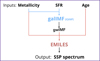 |
Fig. 3. Flowchart of the GalIMF–E-MILES connection. The input data for GalIMF are the metallicity and the SFR, and its output is the gwIMF. E-MILES takes an age, the output gwIMF, and the same metallicity as inputs, then returns as the output the corresponding SSP spectrum. |
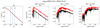 |
Fig. 4. Bottom-heavy IMF case (log10(SFR) = 0; [M/H] = 0.22). Panel (a) shows the number of stars per mass interval. The canonical IMF is in red, and the gwIMF is in black (normalised to have the same mass, as Sect. 2.4 shows). The vertical blue lines represent the mass of the most massive surviving star at 10, 1, and 0.1 Gyr (from left to right). Panels (b), (c), and (d) present the spectra for 0.1, 1, and 10 Gyr, respectively. For the spectra, the canonical IMF is in red and the gwIMF is in black, as before. |
We calculated a database of gwIMF-dependent spectra for the two isochrones, all the ages, and the metallicities available on the E-MILES website. Both the age and metallicity have a fixed range of values due to their empirical basis (see Sect. 2.1 and the E-MILES website for the list of cases). Meanwhile, the SFR can take any input value, though we acknowledge that the recommended values range from 3.5 ⋅ 10−6 to about 104 M⊙ yr−1. Galaxies with an SFR lower than 3.5 ⋅ 10−6 M⊙ yr−1 do not have a correlated and optimally populated star cluster population formed in the galaxy. Without a well-defined embedded star-cluster mass function, such galaxies cannot apply the IGIMF theory (Yan et al. 2020). A galaxy with SFR < 3.5 ⋅ 10−6 M⊙ yr−1 forms 35 M⊙ over δ = 10 Myr in stars and would correspond to an Hα-dark galaxy (Pflamm-Altenburg et al. 2007), which if it were on the main sequence would have a stellar mass near ≈103 M⊙ (Haslbauer et al. 2024, right panel of their figure 7). The gwIMF variation of galaxies with an SFR higher than about 104 M⊙ yr−1 has not yet been validated by observation (Yan et al. 2017; Zhang et al. 2018). The gwIMF-dependent SSP spectral library will be available on the E-MILES website and in the recently presented python module titled “milesPy”. For such a library, we have decided to use the following SFR values: log10(SFR) = [ − 4, −3.5, ...,3.5, 4]. Still, any other SFR value can be queried to calculate a model, if necessary.
2.4. Normalisation
In comparative studies of stellar populations characterised by different stellar IMFs, it is essential to normalise these populations to a consistent and meaningful physical scale. For the analysis presented here, we normalise all stellar populations to their total initial stellar mass. To directly connect this normalisation to a galaxy-wide SFR, we assume that each simple stellar population (SSP) forms with a total mass defined as MSSP = SFR × 10 Myr (Jeřábková et al. 2018); haslbauer2024effect.
We emphasise, however, that different scientific applications might necessitate alternative normalisation strategies. For example, when comparing stellar populations at equivalent SFRs, the relative flux contributions of stars across different mass ranges may guide the normalisation process within each model, reflecting variations in the underlying IMF. Thus, the choice of normalisation approach should always be driven by the specificscientific context and objectives of the study.
3. Stellar population observables
In this section, we explore the influence of considering a gwIMF when producing SSP spectra. We address the changes in the retrieved flux and the behaviour of line-strength indices.
3.1. The spectral flux
To present the effect of the environment-dependent gwIMF on the SSP spectra, we have selected three illustrative data-driven scenarios: bottom-heavy, top-light, and top-heavy IMFs. These cases are shown in Figs. 4, 5 and 6, respectively. We compare the results of these different gwIMF cases with their corresponding model of the canonical IMF based on the Milky Way (Kroupa 2001), keeping the same age and metallicity. In terms of comparing different gwIMF, one should take into account that the SFR is responsible for altering the high-mass segment and the metallicity affects the low-mass one. We chose three different ages to display (0.1, 1, and 10 Gyr) for each one of the different gwIMFs. In these figures, panel (a) is similar to what is shown in Fig. 1. Panels (b), (c), and (d) present the spectra for both cases (as before, red and black) with varying ages for each one of them.
The shift from the canonical IMF to the gwIMF instigates noticeable alterations in the overall spectrum. The differences in the IMF shape affect the spectrum in different ways: the differences in the value between both IMFs change the flux of the spectrum, while the changes in the relative number of stars draw differences between the indices (see Sect. 3.2). This change underscores the influential role of underlying IMF assumptions in shaping the observable outcomes. Before addressing the analysis, it is important to remember two concepts: first, stars more massive than the most massive surviving star at a given age do not contribute to the flux we observe; second, stars with higher masses are more luminous and thus contribute a large fraction of the total flux in the stellar population.
3.1.1. Bottom-heavy IMF: High metallicity and solar SFR
In Fig. 4, we present a bottom-heavy IMF scenario, reflected by an intermediate SFR with high metallicity population (log10(SFR)=0, [M/H] = 0.22). This shape of the gwIMF accounts for a larger amount of low-mass dwarf stars relative to those more massive, although the solar SFR does not alter drastically the high-mass regime of the gwIMF. Observations have shown that massive ETGs often exhibit a bottom-heavy IMF compared to the Milky Way (La Barbera et al. 2016, 2017; Van Dokkum et al. 2017; Parikh et al. 2018; Yan et al. 2024). However, it is important to note that ETGs evolve with time, and therefore, we expect the IMF (dependent on physical conditions like SFR and metallicity) to evolve accordingly (Jeřábková et al. 2018; Yan et al. 2019). Thus, the presented bottom-heavy IMF primarily reflects the present-day snapshot and corresponding conditions.
The three age panels shown in the figure demonstrate that the flux of the canonical IMF consistently exceeds that of the gwIMF. This behaviour can be understood by examining the underlying stellar mass distribution. From approximately 0.65 M⊙ upwards to the mass of the last surviving star, the canonical IMF exhibits an excess of massive stars compared to the gwIMF. Since these massive stars are significantly more luminous, their contribution dominates the total spectral flux. Although the gwIMF predicts a greater number of low-mass stars, their contribution to brightness is relatively minor. The dominance by massive stars explains why the flux difference between the canonical and gwIMF spectra is largest at younger ages, when a greater number of these luminous massive stars are still alive, contributing prominently to the observed flux. Also, we note how the difference between the canonical IMF and the gwIMF spectral flux at older ages is more prominent at longer wavelengths. This range is dominated by low-mass stars, whose contribution is higher in the canonical IMF for old galaxies. We compare the canonical IMF and the gwIMF spectra by inspecting those wavelengths with the approximately highest flux and then calculating the absolute relative difference with respect to the canonical IMF case (|FgwIMF − FIMF − canon|/FIMF − canon). In this case, we find relative differences up to ≈37% for the three ages selected.
3.1.2. Top-light IMF: Solar metallicity and low SFR
In Fig. 5, we study a top-light IMF scenario, represented by a low SFR and an intermediate metallicity (log10(SFR)= − 4, [M/H] = 0.00). This case is characterised by a steeper slope at the high-mass end compared to the canonical IMF, given by a gwIMF where the SFR reduces and limits the number of high-mass stars. Note that the high-mass end of the IMF is primarily driven by the star formation intensity, while metallicity has only a secondary effect. Such a top-light IMF has been observationally associated with environments like dwarf galaxies exhibiting low SFRs (Yan et al. 2020); watts2018star; mucciarelli2021relic. This leads to Hα-deficient galaxies (Pflamm-Altenburg et al. 2007; Pflamm-Altenburg & Kroupa 2008; Lee et al. 2009).
This top-light IMF case serves as an illustrative example of how the spectral flux varies with stellar age. In the 0.1 Gyr panel (b), the spectrum corresponding to the canonical IMF exhibits a higher flux than the gwIMF spectrum. However, for the 1 and 10 Gyr panels (c) and (d), we observe the opposite trend, with the flux difference increasing at older ages.
For the 0.1 Gyr case of panel (b), the spectrum associated with the canonical IMF exhibits a greater flux than the gwIMF-related spectrum. In the range from 2.31 to 5.42 M⊙, the gwIMF remains above the canonical IMF. However, for larger stellar masses, the dominance of the most luminous ultimately determines the overall spectral shape, leading to the observed behaviour.
On the contrary, in panels (c) and (d) an opposite trend is found: the gwIMF remains above the canonical IMF from the initial stellar mass up to the mass of the last surviving star at 10 Gyr (1.06 M⊙), resulting in an excess flux contribution from the gwIMF. Note how, in the 1 Gyr case of panel (c), there exists a mass range (2–2.31 M⊙) where the canonical IMF surpasses the gwIMF, leading to a smaller flux difference between the two spectra. At last, this difference increases in panel (d) and is only due to the difference in the surviving stellar mass, given that both IMFs show a very similar slope and weighting. As in the previous section, we calculate the absolute relative difference with respect to the canonical IMF case, obtaining a variability up to 44% for the 0.1 Gyr case, up to 20% for 1 Gyr and up to 60% for 10 Gyr.
3.1.3. Top-heavy IMF: Low metallicity and high SFR
In Fig. 6, we present a top-heavy IMF scenario, considering high SFR and low metallicity (log10(SFR)=2, [M/H] = −0.4). This case is characterised by a relatively higher proportion of massive stars due to a higher SFR, in comparison to the low-mass region. Such IMFs are typically found in environments with extreme star formation conditions. These include highly star-forming regions in distant galaxies, as suggested by recent James Webb Space Telescope observations indicating top-heavy IMFs at redshifts greater than 10 (Haslbauer et al. 2022; Cameron et al. 2024; Hutter et al. 2025).
The spectra displayed across the three ages highlight the disparity between the canonical IMF and the gwIMF. In all cases shown, the spectrum corresponding to the canonical IMF exceeds that of the gwIMF. This occurs because, in the stellar populations considered (the youngest being 0.1 Gyr), the canonical IMF is above the gwIMF, especially accounting for massive and luminous alive-stars. Ideally, for spectra below 0.1 Gyr, which are not included here due to the limitation of the underlying SPS models, we could expect the discrepancy between IMFs to decrease at first, as we go towards younger ages. At these ages, massive stars that dominate in the gwIMF are still alive, and their contribution increases the gwIMF flux. The difference observed at 0.1 Gyr is primarily due to the higher number of low-mass stars in the canonical IMF. Afterwards, as we move to even younger ages, the contribution from massive stars becomes increasingly significant in the gwIMF. Hence, at some point, the gwIMF associated spectral flux should exceed that of the canonical IMF. Again, we calculate the absolute relative difference, obtaining values up to 37% for the 0.1 Gyr case, up to 60% for 1 Gyr and up to 70% for 10 Gyr.
3.2. Line-strength index sensitivities
Line indices are specific measurements of spectral features, typically defined over narrow wavelength ranges that are designed to isolate the contribution of particular stellar populations or elemental abundances. Despite the increasing use of full spectral fitting techniques, line indices remain widely used due to their robustness, interpretability, and the ease with which they can be compared across different datasets and models. In particular, they provide a convenient way to trace the influence of low and high-mass stars on observed spectra and are less sensitive to uncertainties in flux calibration or dust extinction. Also, indices are especially valuable when working with lower-resolution or noisier data, where fitting the full spectrum may not be reliable.
In this section, we focus on the index sensitivities to varying gwIMF shapes. A way to achieve this is to take as a reference the index values obtained for the canonical IMF (taken as the universal IMF from Kroupa 2001, introduced in Sect. 1 or Fig. 1) and then assess whether the gwIMF-associated index differences can be detected in real galaxy spectra.
Analysing the differences between the gwIMF and the canonical IMF is complex, as multiple factors influence the behaviour of the indices. To clarify this process, we first examined the proportion of stars within different mass ranges for each IMF, which are illustrated in Fig. 1. Next, we investigated how stars contribute to the index by analysing its dependence on stellar parameters. It is important to clarify that while both spectral fluxes and line indices depend on the IMF through the distribution of stellar masses, the analysis of indices is particularly sensitive to the relative contributions of different mass ranges, that is, to the slope or shape of the IMF rather than just the overall number of stars. This contrasts with the spectral flux analysis of the previous section, where the focus was primarily on the total stellar light produced under different IMFs.
We then extended our investigation to determining where the index finds its maximum in relation to different parameters, including luminosity. To provide a comprehensive understanding, we strove to link these index peaks to the temperature and gravity of stars to effectively associate these features with specific types of stars. Once we identified the stars that maximise a particular index, our next step was to determine their associated stellar mass and study the relative number of stars of each IMF in such a range. In some cases, it was necessary to account for stars of high brightness, which might hinder the index performance, among other influencing factors.
The relative number of stars within the IMF holds a significant relevance in our analysis. For instance, when various IMFs share the same relative number of stars, their associated indices do not exhibit significant differences. In other words, galaxies with the same IMF slope have the same index strength. This is shown in the top-light case at 10 Gyr (Fig. 5) both IMFs are parallel in that range of masses, up to 1.06 M⊙. In such cases, there are no differences in any index between the canonical IMF and the gwIMF scenarios, as is shown in the next figures. This method leverages the fact that the total mass of the population is normalised to one. Consequently, a greater abundance of massive stars in one IMF implies a relative scarcity of lower-mass stars in comparison.
We follow this procedure to study key line strengths, as well as assess the extent and regime in which they deviate from the standard canonical IMF. To ensure a comprehensive analysis, we incorporate various representative age and metallicity indicators, along with all IMF-sensitive indices reported within the covered spectral range. Specifically, here we analyse the indices NaD, TiO2(sdss), Mgb, ⟨Fe⟩ and Hβo. Then, in Appendix A we present an extra set of indices we find interesting for the reader: aTiO, bTiO, TiO1, CaH1, CaH2, Mg4780, CN2, C24668, Fe5270, Fe5335, Hβ, HδF, and Hγσ130. These indices have been compiled from multiple sources (Worthey & Ottaviani 1997; Trager et al. 1998; Vazdekis et al. 2001b,a; Serven et al. 2005; Cervantes & Vazdekis 2009; La Barbera et al. 2013; Spiniello et al. 2014), and are calculated via integration, as described in Worthey et al. (1994), with the nominal resolution of the E-MILES spectra (FWHM = 2.51 Å, Vazdekis et al. 2010). To evaluate the extent to which these indices can constrain IMF shapes, we consider typical error bars for signal-to-noise (S/N) ratios of 50 and 100.
We compared the resulting line strengths to those predicted by our reference canonical IMF models, computed at the same metallicity and age. This comparison allowed us to identify which indices are primarily dependent on the gwIMF and to explore the underlying reasons for their variations in different scenarios. From this set of indices, we select a representative subset whose behaviour closely resembles that of the others. Specifically, in Figs. 7 and 8 we show IMF-sensitive indices (NaD and TiO2(sdss), respectively); in Figs. 9 and 10 we show metallicity-sensitive indices (Mgb and ⟨Fe⟩ 6, respectively); and in Fig. 11 we show an age-sensitive index (Hβo). The index values are plotted as a function of age, ranging from 0.063 to 14.1254 Gyr. In all these figures, the top panel presents the index value at each age for both the canonical IMF (black solid line) and gwIMFs with varying SFRs (indicated by the colour bar). These top panels depict the behaviour of each index for the solar metallicity case. The lower panels display the differences between the gwIMF index values and those corresponding to the canonical IMF, for metallicities of [M/H] = −0.4, 0.0, and 0.22 (from top to bottom). Additionally, we include representative observational errors for a signal-to-noise ratio of S/N = 50 (dashed grey line) and S/N = 100 (dotted grey line) to illustrate measurement uncertainties. Before examining each index individually, we could already identify some general trends across all of these figures:
-
First, for solar metallicity and log10(SFR) = 0, the index values corresponding to the canonical IMF and the gwIMF are virtually indistinguishable at all ages, as expected.
-
Second, it is important to note that for old stellar populations, metallicity is the primary driver of the IMF, while the SFR has little influence in the gwIMF scenario. As a result, most differences in the indices at older ages stem from variations in metallicity. For example, at ages of 10 Gyr or older, the most massive surviving star has a mass of approximately 1 M⊙ or lower. In this regime, low-mass dwarf stars dominate the light, and metallicity becomes the key factor shaping the gwIMF. Therefore, if the metallicity is solar ([M/H] = 0), the relative number of stars in both the gwIMF and canonical IMF remains the same, leading to no significant differences in index values. Conversely, for increasingly younger stellar populations, more massive and luminous stars contribute significantly to the index values, making SFR variations the dominant factor. In this regime, if log10(SFR)=0, the differences between the indices associated with the gwIMF and the canonical IMF remain negligible, regardless of metallicity.
-
Third, around 0.1–0.2 Gyr, we observed a distinct gap in the index differences, which is particularly pronounced in metal-poor populations. This separation arises due to the onset of the asymptotic giant branch (AGB) evolutionary phase, which significantly impacts the spectral features of the stellar population. The more pronounced effect at low metallicity may be linked to the fact that metal-poor stars evolve differently, with AGB stars becoming relatively more prominent at these ages. Additionally, in our models, low-metallicity populations tend to form more massive stars under non-canonical IMFs (e.g. due to higher SFRs), which can enhance the AGB contribution and alter the index evolution more markedly.
-
Fourth, in metal-poor populations, the spread in index values between different IMFs is more extended across all ages. This reflects a stronger impact of the IMF variations: Changes in the SFR shape at low metallicities lead to systematically fewer low-mass stars compared to the canonical IMF.
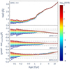 |
Fig. 7. Index information of NaD. Each index panel contains four vertical sub-panels. The first top panel represents the index value (in black based on canonical IMF and with a colour palette based on gwIMF for different SFRs) for a solar metallicity of [M/H] = 0. Similarly, the bottom panels represent the difference between the index based on gwIMF with different SFRs and the one based on the canonical IMF. From the second to the fourth panel, each one represents different metallicities (in order [M/H] = −0.4, [M/H] = 0, [M/H] = 0.22), signalling in each case a representative observational error obtained for a signal-to-noise ratio of S/N = 50 (dashed grey line) and S/N = 100 (dotted grey line). |
3.2.1. NaD and TiO2(sdss) IMF indicators
In Figs. 7 and 8, we analysed NaD and TiO2(sdss) indices, respectively, which are commonly used as IMF indicators (e.g. La Barbera et al. 2013). The NaD index corresponds to a doublet feature located at 5876.875–5909.375 Å, while the TiO2(sdss) index represents a molecular band spanning 6189.625–6272.125 Å. The sensitivity of these indices to the IMF arises from their dependence on different stellar parameters. Spiniello et al. (2014) showed that the NaD index primarily traces surface gravity, as only dwarf stars exhibit an increase in NaD absorption with decreasing temperature. This effect is particularly pronounced for M-dwarfs with Teff ≲ 4000 K. In contrast, for giant stars with log(g)≲1.5 (g in m/s2 units) and similarly low temperatures, the NaD index shows only a modest increase compared to that observed in dwarf stars. For the TiO2(sdss) index, Spiniello et al. (2014) found that it also increases with decreasing temperature, with this trend becoming more significant for stars with Teff ≲ 4000 K, regardless of whether they are giants or dwarfs. Note how the properties of this index are shared with its partner, the TiO1 index, as shown in Appendix A.
In old stellar populations, a steeper IMF slope results in a larger fraction of M-dwarfs, leading to an overall increase in these index values. Additionally, in older populations, the mass of the most massive surviving star decreases, making the contribution of M-dwarfs increasingly significant. Consequently, a bottom-heavier IMF results in a greater relative fraction of cool dwarf stars, further enhancing these index values. For intermediate-age populations, however, the presence of luminous and cool AGB stars in the mass range of 2–6 M⊙ (with log(g)≲1.5), implies that the TiO2(sdss) index increases when the age approaches the onset of this evolutionary phase around 0.1 Gyr. The NaD index does not exhibit a similar trend, as only M-dwarfs contribute to the increase in the strength of this index, but their relative contribution to the integrated light of the stellar population lowers with decreasing age.
When comparing the line-strength differences predicted by a canonical IMF and gwIMFs in the old age regime (≳3 Gyr), the relative number of M-dwarfs in each IMF plays a crucial role, as the most massive surviving stars have masses around ≤1 M⊙. In this context, for stellar populations of sub-solar metallicity we expect lower index values in the gwIMF compared to the canonical IMF, resulting in a negative difference in the corresponding panels of both figures. This effect arises because the canonical IMF favours a higher abundance of M-dwarf stars at [M/H] = −0.4. Conversely, for stellar populations with super-solar metallicity ([M/H] = 0.22), the NaD and TiO2(sdss) indices exhibit higher values in the gwIMF case, leading to a positive difference.
For younger ages, variations in the SFR significantly affect the line-strength indices when comparing the differences between these two IMF prescriptions. On the one hand, as age decreases, the mass of the most massive surviving star increases, enhancing the relative contribution of bright and cool AGB stars. On the other hand, a higher SFR leads to a greater presence of luminous AGB stars, which play a key role in driving these variations, particularly for the TiO2(sdss) index. Therefore, in Figs. 7 and 8, the difference in the indices is positive for young ages and high SFRs. On the contrary, lower SFRs lead to decreased gwIMF index values with respect to the canonical IMF case.
Measuring the differences shown in Fig. 7 for the NaD index is particularly challenging. We estimate that a signal-to-noise ratio (S/N) of at least 100 is required for reliable measurements, and its applicability is mostly limited to young or very old ages. For example, for solar metallicity ([M/H] = 0.0) and ages below 0.1 Gyr, the NaD index shows variations up to 0.2 Å when comparing the canonical IMF to the gwIMF with the lowest and highest endmost SFRs (log10(SFR) = −4 and 4). In contrast, the differences in the TiO2(sdss) index can be measured with good-quality spectra at an S/N above 50 and remain accessible across nearly all ages. This index demonstrates measurable differences up to ≈0.01 magnitudes at intermediate and young ages, emphasising its sensitivity to changes in stellar populations driven by the gwIMF.
3.2.2. Mgb and ⟨Fe⟩ metallicity indicators
The metallicity indicators Mgb (5160.125–5192.625 Å) and the mean iron7 ⟨Fe⟩ (≈5245.65–5352.125 Å) are shown in Figs. 8 and 9, respectively. Both indices increase in strength with decreasing temperature and increasing metallicity for both dwarf and giant stars (Gorgas et al. 1993). However, these authors also showed that the temperature dependence is more pronounced for dwarf stars in the case of the Mgb index, whereas the ⟨Fe⟩ index exhibits a stronger sensitivity to metallicity, particularly for the two iron lines it comprises. Therefore, the effect of gravity is more relevant for the Mgb index: higher surface gravity (e.g. of M-dwarfs) leads to higher gas pressure, which affects the wings of the index by making them the deeper and broader and thus enhancing the index (Schiavon et al. 2002). For further investigation, in Appendix A, we present a variety of alternative abundance-sensitive indices.
Consequently, due to their dependence on stellar parameters, the strengths of both indices increase with age and metallicity. At older ages, as the mass of the most massive surviving star decreases, M-dwarfs begin to influence the Mgb index. This effect arises because the Mgb index is more sensitive to gravity compared to ⟨Fe⟩. Meanwhile, the latter is more sensitive to metallicity and remains largely unaffected for old ages. At super-solar metallicity, the higher relative fraction of M-dwarfs leads to larger Mgb index values for the gwIMF, whereas at subsolar metallicity, the Mgb index values are lower. In this age regime, the differences in the Mgb index between the gwIMF and the canonical IMF are challenging to detect unless very high quality data with S/N exceeding 50 is available. At the endmost SFRs, the Mgb index can show noticeable variations up to 0.1 Å for metal-poor stellar populations below 1 Gyr. At younger ages, the SFR, which governs the massive end of the gwIMF, leads to some differences compared to the canonical IMF. These variations arise from the relative proportion of luminous, cool evolved AGB stars (which is higher for greater SFRs), with their effects becoming more pronounced as the population approaches the onset of this phase around 0.1 Gyr. However, most of these differences remain undetectable. In the case of the ⟨Fe⟩, some differences can be detected for ages below 1 Gyr (up to ≈0.1 Å, with an available S/N of at least 50), specially in low-metallicity regimes.
Following these results, it is worth noting that indices such as Mgb and ⟨Fe⟩ are ideal for studying the properties of a stellar population without being significantly affected by IMF variations. This can be useful when the intention is to study solely the metallicity of an object, without IMF variations interfering.
3.2.3. Hβo optimised age indicator
Finally, in Fig. 11, we present a similar analysis for the Hβo index (4839.275–4877.097 Å). This index has been optimised to be partially insensitive to metallicity, while maximising its sensitivity to age (Cervantes & Vazdekis 2009). Like Hβ and the higher-order Balmer line indices, it is commonly used as an age indicator for stellar populations. The highest values of these Balmer lines are associated with hotter temperatures, peaking in the range of ≈8000–10 000 K (Gorgas et al. 1993; Worthey & Ottaviani 1997). At all metallicities, the turn-off stars are the main contributors to this index, due to being the hottest in the stellar population. However, at very low metallicities, where the Horizontal Branch extends towards the blue, these stars also enhance the index value. Notice how the rest of the Balmer lines share a similar behaviour, as shown in Appendix A. Numerically, the Hβo index can vary by roughly 0.1 Å up to 1 Å when moving towards younger populations. Notice that, larger differences appear for the lowest SFRs than the highest. The first detectable differences between the canonical IMF and the gwIMF appear at 2 Gyr for sub-solar populations and at 0.2 Gyr for super-solar populations. However, for older populations, differences between gwIMF and canonical IMF indices become negligible, often falling below detectable thresholds.
The peak of the index at ≈8000–10 000 K corresponds to stars with masses of approximately 3.5 M⊙, which is associated with an age of around ≈0.3 Gyr. This corresponds to the highest index value found in the first panel of Fig. 11, while both younger and older ages exhibit lower index strengths.
For ages older than 1–2 Gyr, low-mass turn-off stars dominate the strength of the Hβo index. As a result, the differences between the canonical IMF and the gwIMF, regardless of the SFR, become indistinguishable and remain close to zero. This trend is observed across the metallicity range shown in Fig. 11, as the horizontal branch extends towards the blue only at lower metallicities.
We find differences in the index values between these two IMF shapes at younger ages, with some cases being detectable for S/N around 100. However, the observed differences between these IMF shapes are in the opposite direction compared to those found for the NaD, TiO2(sdss), Mgb, and ⟨Fe⟩ indices discussed earlier. These differences are particularly pronounced at the youngest ages shown in Fig. 11. This can be attributed to the fact that, for higher SFRs, the resulting gwIMF yields a relatively higher fraction of luminous stars with masses above ≈3.5 M⊙, leading to a decrease in the Hβo index value. For instance, within this mass range, the proportion of ≈3.5 M⊙ stars in the canonical IMF is greater than that found in the gwIMF with log10(SFR) = 2.
Other Balmer lines, such as the Hγ and Hδ, are also widely used as reliable age indicators. These higher-order Balmer lines offer a practical alternative to Hβo, as they tend to be less impacted by emission fill-in, making them valuable for resolving ages in both young and intermediate-age stellar populations. The Dn4000 index is another critical tool, primarily serving as a broken indicator around 4000 Å. The strength of this feature increases with the age of the stellar population because of the build-up of metal lines, providing a sensitive measure of age that is particularly useful in older systems where IMF effects diminish.
4. Discussion and potential applications
In Sect. 3.2, we characterised the impact of representative gwIMF shapes, driven by variations in SFR and metallicity, on a set of commonly used IMF, metallicity, and age-sensitive indices in the optical range. The selected indices illustrate the behaviour of other indices with similar sensitivities to relevant stellar population parameters within this spectral range. Aside to those presented above, other IMF-sensitive optical indices include aTiO, bTiO, TiO1, CaH1, CaH2, and Mg4780. Additional optical abundance indicators include CN2, C24668, Fe5270, and Fe5335, while the Balmer lines HδF, Hγσ130, Hβ serve as age indicators (see Appendix A).
This study can also be extended to other spectral ranges outside the MILES wavelengths. For simplicity, this work only focuses on the optical range (3540–7410 Å); however, the full GalIMF–E-MILES library we provide allows for the study of the bluer (down to 1680 Å) and redder (up to 50 000 Å) parts of the spectrum, too. Some interesting information might be found there, so let us give an example. In the near infrared, certain indices have demonstrated sensitivity to IMF variations, as the Ca II triplet (CaT) index, which covers the wavelength region around 8498, 8542, and 8662 Å. This index is gravity-sensitive (Cenarro et al. 2001) and tends to show lower values for steeper IMF slopes in stellar populations (Vazdekis et al. 2003; Smith et al. 2015). Another key near infrared indicator is the FeHWing-Ford index, centred on the absorption band around 9916 Å. The strength of this index is significantly influenced by the contribution of cool, metal-rich dwarfs and giants, making it particularly useful for probing IMF variations and identifying the relative abundance of low-mass stars in a population (Wing & Ford 1969). Moreover, this index has been shown to have the potential to distinguish the shape of the IMF at the low-mass end (La Barbera et al. 2016). Another set of promising Na- and IMF-sensitive features are the Na I lines found in the I (8190 Å), J (1.14 μm), and K (2.21 μm) bands (Smith et al. 2015; La Barbera et al. 2017).
The integration of the GalIMF–E-MILES codes provides a robust framework for generating both simple and composite stellar population models that incorporate variable IMFs, reflecting different SFHs and chemical evolution scenarios. This advancement enables several potential applications and future research directions:
-
Generation of mock composite stellar population spectra: using the newly synthesised GalIMF–E-MILES library, it is possible to construct mock composite stellar population spectra with predefined SFHs representative of galaxies across a wide range of masses. This allows for realistic synthetic galaxy spectra that facilitate testing spectral fitting algorithms and refining methodologies to accurately recover input SFHs. A key aspect is that these mock spectra are essential to quantify and disentangle the effects of IMF variations from other stellar population parameters (e.g. Ferreras et al. 2015). A similar tool has already been presented with theoretical stellar spectra (Zonoozi et al. 2025).
-
Empirical validation through spectral fitting: applying the GalIMF–E-MILES spectral library enables fitting observed galaxy spectra using models incorporating variable IMFs. By comparing the derived galaxy properties (e.g. stellar mass, age, metallicity, SFH, chemical enrichment) with those obtained using standard IMF assumptions, we can directly assess how IMF variability impacts our interpretation of galaxy evolution (e.g. Vazdekis et al. 1996; Weidner et al. 2013; Jeřábková et al. 2018).
-
Observational signatures in key spectral features: specific line-strength indices, as the ones addressed here, or colours sensitive to the high-mass or low-mass ends of the IMF can be examined using the GalIMF–E-MILES library. Identifying these observational signatures allowed us to empirically validate theoretical IMF variation predictions and test these against observational data, improving the consistency between theory and observation. Not only can the shape of the IMF be robustly investigated, but also its functional form, at least at the low-mass end (e.g. La Barbera et al. 2016; Lyubenova et al. 2016; Eftekhari et al. 2021).
-
Impact in the interpretation of young stellar populations: when fitting unresolved stellar populations, the application of the gwIMF models to the analysis of stellar populations could lead to different outcomes compared to using a standard, fixed IMF, with direct consequences for the estimation of galaxy masses and ages. For instance, when inspecting young populations, the variations introduced by different SFR or gwIMF, while noticeable, are often dominated by even small changes in age. This effect can be quantified by examining how each index (e.g. the Hβo) varies under different SFR or gwIMF assumptions, and comparing the resulting change to the equivalent variation caused by a shift in age. In doing so, one can determine the age difference that would produce a similar effect on the indices, providing a useful sense of the relative impact of IMF versus age in shaping the spectral features of young stellar populations. On the other hand, a combination of key index indicators should be able to break these degeneracies when deriving the metallicity, age and SFR (and its gwIMF accordingly) of a stellar population.
-
Modelling stellar populations of ETGs: variations in the IMF have been reported for ETGs, both as a function of galaxy mass (e.g. La Barbera et al. 2013) and within individual galaxies, particularly in the most massive ones (e.g. Martín-Navarro et al. 2015). Additionally, time-dependent IMF variations have been proposed, reflecting the evolving SFH and chemical enrichment of these systems (e.g. Vazdekis et al. 1997; Weidner et al. 2013; Jeřábková et al. 2018). Given these findings, ETGs are prime candidates for modelling with the GalIMF–E-MILES library. Such studies will enable us to test whether the observed present-day spectral features align with theoretical predictions in a self-consistent manner.
-
Implications for galaxy chemical evolution: IMF variability directly affects the available mass budget to form new stars and influences the rates of supernova explosions and thus the chemical enrichment processes. By using IMFs responsive to physical conditions such as SFR and metallicity, models can better constrain chemical enrichment histories, as well as the interplay between stellar evolution and interstellar medium chemistry (e.g. Ferreras et al. 2015; Yan et al. 2021). This provides insights into galaxy enrichment histories and future observational strategies.
In summary, the combination of E-MILES SPS code with the GalIMF code predictions significantly advances our ability to study and interpret galaxy properties through the lens of IMF variability. These applications promise new paths for understanding galaxy formation and evolution, enhancing the predictive power and interpretative capability of current and future observations.
5. Conclusions
In this study, we have successfully implemented, for the first time, an environment-dependent variable stellar IMF into the E-MILES evolutionary SPS code. We summarise our main contributions and conclusions as follows:
-
We have presented an extensive library of SSP spectra at moderately high resolution computed with the E-MILES framework and based on empirical stellar libraries. Our models incorporate variable gwIMFs derived from the IGIMF theory and capture systematic variations with key physical parameters such as age, SFR, and metallicity.
-
Our newly generated spectral library integrating variable IMF scenarios into E-MILES is publicly available through the E-MILES website and via the python module milesPy. Researchers can freely access and utilise these models to investigate the effects of IMF variability on stellar populations and galaxy properties.
-
We have demonstrated that varying the gwIMF produces direct, observable impacts on the spectral energy distributions of stellar populations, influencing interpretations of galaxy properties from observational data. By comparing gwIMF-based models to those assuming a canonical IMF, we showed how IMF variability alters spectral flux distributions across different stellar ages, with particularly prominent effects at young ages when massive stars dominate the spectral output. When comparing the canonical IMF and the gwIMF spectra, we found relative differences of 37% and up to 70%, depending on the spectral region and scenario selected. Not only does the flux diverge between both cases, sometimes the order for which one is brighter is interchanged.
-
Additionally, we investigated the impact of adopting a gwIMF versus a canonical IMF on key absorption line-strength indices. Our results reveal that while some indices behave similarly under both IMF scenarios, others exhibit clear and measurable differences. We find that, for the endmost SFRs in the gwIMF, the NaD, TiO2(sdss) and Hβo indices can be good indicators for detecting measurable differences between both IMF cases, while the metallicity indicators, Mgb and ⟨Fe⟩, remain largely insensitive. For instance, this is clearly shown in the TiO2(sdss) index, which exhibits measurable differences up to 0.01 magnitudes under endmost SFR conditions. The Hβo index also shows remarkable differences (from 0.1 to 1 Å) above typical S/N requirements for ages below 2 Gyr for metal-poor populations and 0.2 Gyr for metal-rich populations. These divergences provide powerful diagnostic tools for empirically testing IMF variability predictions against observational data.
This study highlights the importance of incorporating realistic environment-dependent IMFs into SPS models. Approaches such as the one presented here are essential for advancing our understanding of galaxy evolution and for interpreting observational data with greater physical accuracy. In summary, our findings underscore the necessity of sophisticated, physically motivated modelling frameworks to unravel the complex interplay between IMF variability and galaxy evolution, setting the stage for further observational and theoreticalexploration.
Data availability
E-MILES SSP model spectra based on variable galaxy-wide IMFs (gwIMFs) are available in the python module “milesPy” (https://github.com/miles-iac/milespy). Additionally, this library is publicly available at the E-MILES website (http://miles.iac.es), under the tag: “Other predictions/data”. As we expect to update the website in the near future, this address might change. The GalIMF python3 code is available at: https://github.com/Azeret/GalIMF.
Acknowledgments
First, we want to thank Miguel Cerviño for the insightful conversations into the puzzling depths of stellar population statistics, as well as Mike Beasley for the new perspectives and wise advice. Special thanks to Javier Sánchez Sierras for his teachings and Isaac Alonso Asensio for helping with the milesPy implementation. AV and PRB acknowledge support from grant PID2022-140869NB-I00 from the Spanish Ministry of Science and Innovation. Also, AV and SY acknowledge support from grant PID2021-123313NA-I00 from the Spanish Ministry of Science, Innovation, and Universities MCIU. This work has also been supported through the IAC project TRACES, which is partially supported through the state budget and the regional budget of the Consejería de Economía, Industria, Comercio y Conocimiento of the Canary Islands Autonomous Community. SY acknowledges support from the ACIISI, Consejería de Economía, Conocimiento y Empleo del Gobierno de Canarias and the European Regional Development Fund (ERDF) under grant with reference ProID2021010079. Part of this work was supported by the German Deutsche Forschungsgemeinschaft, DFG project number Ts 17/2–1. TJ acknowledges the MUNI Award in Science and Humanities MUNI/I/1762/2023. ZY acknowledges the support from the National Natural Science Foundation of China under grant No. 12203021. AHZ is supported by an Alexander von Humboldt Foundation postdoctoral research fellowship. PK acknowledges support through the DAAD Eastern-European at Bonn-Prague exchange programme. This paper made use of the IAC Supercomputing facility HTCondor (http://research.cs.wisc.edu/htcondor/), partly financed by the Ministry of Economy and Competitiveness with FEDER funds, code IACA13-3E-2493. We acknowledge the help from the members of the SIE team of IAC.
References
- Alonso, A., Arribas, S., & Martínez-Roger, C. 1999, A&AS, 140, 261 [NASA ADS] [CrossRef] [EDP Sciences] [Google Scholar]
- Alonso-Herrero, A., Ward, M. J., & Kotilainen, J. K. 1996, MNRAS, 278, 902 [NASA ADS] [Google Scholar]
- Banerjee, S., Kroupa, P., & Oh, S. 2012, MNRAS, 426, 1416 [NASA ADS] [CrossRef] [Google Scholar]
- Bruzual, G., & Charlot, S. 2003, MNRAS, 344, 1000 [NASA ADS] [CrossRef] [Google Scholar]
- Byrne, C. M., Eldridge, J. J., & Stanway, E. R. 2025, MNRAS, 537, 2433 [Google Scholar]
- Cameron, A. J., Katz, H., Witten, C., et al. 2024, MNRAS, 534, 523 [NASA ADS] [CrossRef] [Google Scholar]
- Cassisi, S., Salaris, M., Castelli, F., & Pietrinferni, A. 2004, ApJ, 616, 498 [NASA ADS] [CrossRef] [Google Scholar]
- Cenarro, A., Cardiel, N., Gorgas, J., et al. 2001, MNRAS, 326, 959 [NASA ADS] [CrossRef] [Google Scholar]
- Cervantes, J., & Vazdekis, A. 2009, MNRAS, 392, 691 [NASA ADS] [CrossRef] [Google Scholar]
- Chabrier, G. 2001, ApJ, 554, 1274 [NASA ADS] [CrossRef] [Google Scholar]
- Chabrier, G. 2003, PASP, 115, 763 [Google Scholar]
- Conroy, C. 2013, ARA&A, 51, 393 [NASA ADS] [CrossRef] [Google Scholar]
- Conroy, C., Gunn, J. E., & White, M. 2009, ApJ, 699, 486 [Google Scholar]
- Cushing, M. C., Rayner, J. T., & Vacca, W. D. 2005, ApJ, 623, 1115 [Google Scholar]
- Eftekhari, E., Vazdekis, A., & La Barbera, F. 2021, MNRAS, 504, 2190 [CrossRef] [Google Scholar]
- Eldridge, J., Stanway, E., Xiao, L., et al. 2017, PASA, 34 [Google Scholar]
- Ferreras, I., Barbera, F. L., Rosa, I. G. D. I., et al. 2013, MNRAS, 429, L15 [NASA ADS] [CrossRef] [Google Scholar]
- Ferreras, I., Weidner, C., Vazdekis, A., & La Barbera, F. 2015, MNRAS, 448, L82 [NASA ADS] [CrossRef] [Google Scholar]
- Fontanot, F., De Lucia, G., Hirschmann, M., et al. 2016, MNRAS, 464, 3812 [Google Scholar]
- Gargiulo, I. D., Cora, S. A., Padilla, N. D., et al. 2015, MNRAS, 446, 3820 [Google Scholar]
- Geha, M., Brown, T. M., Tumlinson, J., et al. 2013, ApJ, 771, 29 [NASA ADS] [CrossRef] [Google Scholar]
- Girardi, L., Bressan, A., Bertelli, G., & Chiosi, C. 2000, A&AS, 141, 371 [NASA ADS] [CrossRef] [EDP Sciences] [Google Scholar]
- Gorgas, J., Faber, S., Burstein, D., et al. 1993, ApJS, 86, 153 [NASA ADS] [CrossRef] [Google Scholar]
- Gregg, M., Silva, D., Rayner, J., et al. 2006, The 2005 HST Calibration Workshop: Hubble After the Transition to Two-Gyro Mode, 209 [Google Scholar]
- Grevesse, N., & Noels, A. 1993, in Origin and Evolution of the Elements, eds. N. Prantzos, E. Vangioni-Flam, & M. Casse, 15 [Google Scholar]
- Gunawardhana, M. L., Hopkins, A. M., Sharp, R. G., et al. 2011, MNRAS, 415, 1647 [NASA ADS] [CrossRef] [Google Scholar]
- Haslbauer, M., Kroupa, P., Zonoozi, A. H., & Haghi, H. 2022, ApJL, 939, L31 [Google Scholar]
- Haslbauer, M., Yan, Z., Jerabkova, T., et al. 2024, A&A, 689, A221 [NASA ADS] [CrossRef] [EDP Sciences] [Google Scholar]
- Hennebelle, P., & Grudić, M. Y. 2024, ARA&A, 62 [Google Scholar]
- Hutter, A., Cueto, E. R., Dayal, P., et al. 2025, A&A, 694, A254 [NASA ADS] [CrossRef] [EDP Sciences] [Google Scholar]
- Jeřábková, T., Zonoozi, A. H., Kroupa, P., et al. 2018, A&A, 620, A39 [NASA ADS] [CrossRef] [EDP Sciences] [Google Scholar]
- Koekemoer, A. M., Goudfrooij, P., & Dressel, L. L. 2006, The 2005 HST Calibration Workshop: Hubble After the Transition to Two-Gyro Mode [Google Scholar]
- Kroupa, P. 2001, MNRAS, 322, 231 [NASA ADS] [CrossRef] [Google Scholar]
- Kroupa, P. 2002, Science, 295, 82 [Google Scholar]
- Kroupa, P., & Weidner, C. 2003, ApJ, 598, 1076 [NASA ADS] [CrossRef] [Google Scholar]
- Kroupa, P., Tout, C. A., & Gilmore, G. 1993, MNRAS, 262, 545 [NASA ADS] [CrossRef] [Google Scholar]
- Kroupa, P., Weidner, C., Pflamm-Altenburg, J., et al. 2013, in Planets Stars and Stellar Systems (Springer) 115 [Google Scholar]
- Kroupa, P., Gjergo, E., Jerabkova, T., & Yan, Z. 2024, ArXiv e-prints [arXiv:2410.07311] [Google Scholar]
- La Barbera, F., Ferreras, I., Vazdekis, A., et al. 2013, MNRAS, 433, 3017 [Google Scholar]
- La Barbera, F., Vazdekis, A., Ferreras, I., et al. 2016, MNRAS, 457, 1468 [Google Scholar]
- La Barbera, F., Vazdekis, A., Ferreras, I., et al. 2017, MNRAS, 464, 3597 [Google Scholar]
- La Barbera, F., Vazdekis, A., Ferreras, I., et al. 2019, MNRAS, 489, 4090 [Google Scholar]
- La Barbera, F., Vazdekis, A., Ferreras, I., & Pasquali, A. 2021, MNRAS, 505, 415 [NASA ADS] [CrossRef] [Google Scholar]
- Lee, J. C., De Paz, A. G., Tremonti, C., et al. 2009, ApJ, 706, 599 [NASA ADS] [CrossRef] [Google Scholar]
- Leitherer, C., & Ekström, S. 2011, IAU, 7, 2 [Google Scholar]
- Leitherer, C., Schaerer, D., Goldader, J. D., et al. 1999, ApJS, 123, 3 [Google Scholar]
- Li, J., Liu, C., Zhang, Z.-Y., et al. 2023, Nature, 613, 460 [NASA ADS] [CrossRef] [Google Scholar]
- Lonoce, I., Freedman, W., & Feldmeier-Krause, A. 2023, ApJ, 948, 65 [NASA ADS] [CrossRef] [Google Scholar]
- Lyubenova, M., Martín-Navarro, I., Van de Ven, G., et al. 2016, MNRAS, 463, 3220 [Google Scholar]
- Marks, M., Kroupa, P., Dabringhausen, J., & Pawlowski, M. S. 2012, MNRAS, 422, 2246 [NASA ADS] [CrossRef] [Google Scholar]
- Martín-Navarro, I., & Vazdekis, A. 2024, A&A, 691, L10 [NASA ADS] [CrossRef] [EDP Sciences] [Google Scholar]
- Martín-Navarro, I., Vazdekis, A., La Barbera, F., et al. 2015, ApJ, 806, L31 [CrossRef] [Google Scholar]
- Martín-Navarro, I., Lyubenova, M., Van De Ven, G., et al. 2019, A&A, 626, A124 [NASA ADS] [CrossRef] [EDP Sciences] [Google Scholar]
- Martín-Navarro, I., Pinna, F., Coccato, L., et al. 2021, A&A, 654, A59 [NASA ADS] [CrossRef] [EDP Sciences] [Google Scholar]
- Miller, G. E., & Scalo, J. M. 1979, ApJS, 41, 513 [Google Scholar]
- Mucciarelli, A., Massari, D., Minelli, A., et al. 2021, Nature Astronomy, 5, 1247 [Google Scholar]
- Palla, M., Calura, F., Matteucci, F., et al. 2020, MNRAS, 494, 2355 [NASA ADS] [CrossRef] [Google Scholar]
- Parikh, T., Thomas, D., Maraston, C., et al. 2018, MNRAS, 477, 3954 [Google Scholar]
- Pflamm-Altenburg, J., & Kroupa, P. 2008, Nature, 455, 641 [Google Scholar]
- Pflamm-Altenburg, J., & Kroupa, P. 2009, ApJ, 706, 516 [NASA ADS] [CrossRef] [Google Scholar]
- Pflamm-Altenburg, J., Weidner, C., & Kroupa, P. 2007, ApJ, 671, 1550 [NASA ADS] [CrossRef] [Google Scholar]
- Pflamm-Altenburg, J., Weidner, C., & Kroupa, P. 2009, MNRAS, 395, 394 [CrossRef] [Google Scholar]
- Pietrinferni, A., Cassisi, S., Salaris, M., & Castelli, F. 2004, ApJ, 612, 168 [Google Scholar]
- Rayner, J. T., Cushing, M. C., & Vacca, W. D. 2009, ApJS, 185, 289 [Google Scholar]
- Romano, D., Matteucci, F., Zhang, Z.-Y., Papadopoulos, P., & Ivison, R. 2017, MNRAS, 470, 401 [NASA ADS] [CrossRef] [Google Scholar]
- Salpeter, E. E. 1955, ApJ, 121, 161 [Google Scholar]
- Sánchez-Blázquez, P., Peletier, R., Jiménez-Vicente, J., et al. 2006, MNRAS, 371, 703 [CrossRef] [Google Scholar]
- Scalo, J. M. 1986, Fundamen. Cosmic Phys., 11, 1 [Google Scholar]
- Schiavon, R. P., Faber, S., Castilho, B. V., & Rose, J. A. 2002, ApJ, 580, 850 [Google Scholar]
- Schmidt, M. 1959, ApJ, 129, 243 [NASA ADS] [CrossRef] [Google Scholar]
- Schneider, F., Sana, H., Evans, C., et al. 2018, Science, 359, 69 [NASA ADS] [CrossRef] [Google Scholar]
- Serven, J., Worthey, G., & Briley, M. M. 2005, ApJ, 627, 754 [NASA ADS] [CrossRef] [Google Scholar]
- Smith, R. J. 2020, ARA&A, 58, 577 [NASA ADS] [CrossRef] [Google Scholar]
- Smith, R. J., Alton, P. D., Lucey, J. R., Conroy, C., & Carter, D. 2015, MNRAS, 454 [Google Scholar]
- Spiniello, C., Trager, S., Koopmans, L. V., & Conroy, C. 2014, MNRAS, 438, 1483 [NASA ADS] [CrossRef] [Google Scholar]
- Stanway, E. R. 2020, Galaxies, 8, 6 [Google Scholar]
- Tinsley, B. M. 1968, ApJ, 151, 547 [Google Scholar]
- Tinsley, B. M., & Gunn, J. E. 1976, ApJ, 203, 66 [Google Scholar]
- Trager, S., Worthey, G., Faber, S., Burstein, D., & González, J. J. 1998, ApJS, 116, 1 [NASA ADS] [CrossRef] [Google Scholar]
- Valdes, F., Gupta, R., Rose, J. A., Singh, H. P., & Bell, D. J. 2004, ApJS, 152, 251 [Google Scholar]
- van Dokkum, P. G., & Conroy, C. 2010, Nature, 468, 940 [Google Scholar]
- Van Dokkum, P., Conroy, C., Villaume, A., Brodie, J., & Romanowsky, A. J. 2017, ApJ, 841, 68 [NASA ADS] [CrossRef] [Google Scholar]
- Vazdekis, A., Casuso, E., Peletier, R., & Beckman, J. 1996, ApJ, 106, 307 [Google Scholar]
- Vazdekis, A., Peletier, R., Beckman, J., & Casuso, E. 1997, ApJS, 111, 203 [CrossRef] [Google Scholar]
- Vazdekis, A., Kuntschner, H., Davies, R. L., et al. 2001a, ApJ, 551, L127 [Google Scholar]
- Vazdekis, A., Salaris, M., Arimoto, N., & Rose, J. A. 2001b, ApJ, 549, 274 [Google Scholar]
- Vazdekis, A., Cenarro, A., Gorgas, J., Cardiel, N., & Peletier, R. 2003, MNRAS, 340, 1317 [NASA ADS] [CrossRef] [Google Scholar]
- Vazdekis, A., Sánchez-Blázquez, P., Falcón-Barroso, J., et al. 2010, MNRAS, 404, 1639 [NASA ADS] [Google Scholar]
- Vazdekis, A., Coelho, P., Cassisi, S., et al. 2015, MNRAS, 449, 1177 [Google Scholar]
- Vazdekis, A., Koleva, M., Ricciardelli, E., Röck, B., & Falcón-Barroso, J. 2016, MNRAS, 463, 3409 [Google Scholar]
- Vazdekis, A., Cerviño, M., Montes, M., Martín-Navarro, I., & Beasley, M. 2020, MNRAS, 493, 5131 [NASA ADS] [CrossRef] [Google Scholar]
- Watts, A. B., Meurer, G. R., Lagos, C. D., et al. 2018, MNRAS, 477, 5554 [NASA ADS] [CrossRef] [Google Scholar]
- Weidner, C., Ferreras, I., Vazdekis, A., & La Barbera, F. 2013, MNRAS, 435, 2274 [NASA ADS] [CrossRef] [Google Scholar]
- Weidner, C., & Kroupa, P. 2005, ApJ, 625, 754 [NASA ADS] [CrossRef] [Google Scholar]
- Wing, R. F., & Ford, W. K., Jr 1969, PASP, 81, 527 [CrossRef] [Google Scholar]
- Worthey, G., Faber, S., Gonzalez, J. J., & Burstein, D. 1994, ApJS, 94, 687 [NASA ADS] [CrossRef] [Google Scholar]
- Worthey, G., & Ottaviani, D. 1997, ApJS, 111, 377 [CrossRef] [Google Scholar]
- Yan, Z., Jerabkova, T., & Kroupa, P. 2017, A&A, 607, A126 [NASA ADS] [CrossRef] [EDP Sciences] [Google Scholar]
- Yan, Z., Jerabkova, T., Kroupa, P., & Vazdekis, A. 2019, A&A, 629, A93 [NASA ADS] [CrossRef] [EDP Sciences] [Google Scholar]
- Yan, Z., Jerabkova, T., & Kroupa, P. 2020, A&A, 637, A68 [NASA ADS] [CrossRef] [EDP Sciences] [Google Scholar]
- Yan, Z., Jeřábková, T., & Kroupa, P. 2021, A&A, 655, A19 [NASA ADS] [CrossRef] [EDP Sciences] [Google Scholar]
- Yan, Z., Jerabkova, T., & Kroupa, P. 2023, A&A, 670, A151 [NASA ADS] [CrossRef] [EDP Sciences] [Google Scholar]
- Yan, Z., Li, J., Kroupa, P., et al. 2024, ApJ, 969, 95 [NASA ADS] [CrossRef] [Google Scholar]
- Zhang, Z.-Y., Romano, D., Ivison, R., Papadopoulos, P. P., & Matteucci, F. 2018, Nature, 558, 260 [NASA ADS] [CrossRef] [Google Scholar]
- Zhou, S., Mo, H., Li, C., et al. 2019, MNRAS, 485, 5256 [Google Scholar]
- Zonoozi, A. H., Haghi, H., & Kroupa, P. 2025, MNRAS, 537, 2782 [Google Scholar]
Appendix A: Behaviour of additional line-strength indices
In this appendix, we present an extra set of indices we find interesting for the reader. The interpretation of each index behaviour should be analogous to the one performed in Sect. 3.2. Due to their sensitivity to variations of the IMF, we select aTiO, bTiO, TiO1, CaH1, CaH2 and Mg4780. As abundance or metallicity indicators we include CN2, C24668, Fe5270, and Fe5335. As age indicators, we display the Balmer lines: HδF, Hγσ130 and Hβ.
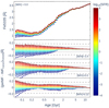 |
Fig. A.10. Abundance indicator: Fe5335. Same labels as in Fig. 7. |
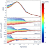 |
Fig. A.11. Age indicator: Hβ. Same labels as in Fig. 7. |
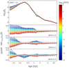 |
Fig. A.12. Age indicator: HδF. Same labels as in Fig. 7. |
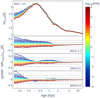 |
Fig. A.13. Age indicator: Hγσ130. Same labels as in Fig. 7. |
Throughout this paper, the SFR is defined in units of M⊙/yr.
Throughout this work, ‘SFR’ refers to the average SFR over the most recent 10 Myr for which we assume galaxies create a new cycle of formed stars (Jeřábková et al. 2018).
E-MILES model predictions are publicly available at http://miles.iac.es/ and through the recently released python module milesPy (https://github.com/miles-iac/milespy).
In the BaSTI isochrones, solar metallicity is taken as [M/H] = 0.06, accounting for the initial metallicity of the Sun under atomic diffusion considerations. This value deviates slightly from the canonical zero-point solar metallicity, resulting in a modest steepening of the low-mass end of the IMF. The solar metallicity is defined according to the Grevesse & Noels (1993) metal mixture, which underlies the BaSTI and Padova00 isochrones used in EMILES.
 .
.
Composed by the Fe5270 and Fe5335, which we show individually in the Appendix A, although they behave similarly to index ⟨Fe⟩.
All Figures
|
Fig. 1. Collection of IMFs (normalised to have the same mass). Columns correspond to log10(SFR) = −2, 0 and 2. Each panel shows the number of stars per mass interval: canonical IMF in red and gwIMF in a gradient of greys for each metallicity ([M/H] = −0.4, 0, and 0.22), from lightest to darkest. The vertical blue lines represent the mass of the most massive surviving star when the age of the population is 10, 1, and 0.1 Gyr, corresponding to ≈1.1, 2.3 and 5.4 M⊙ in each case (assuming solar metallicity). We note that only stars with masses lower than the mass of the most massive surviving star will contribute to the spectra, as the horizontal arrows of the first panel show. The normalisation is performed as explained in Sect. 2.4. |
| In the text | |
|
Fig. 2. Masses of the most massive surviving stars according to the age of the population. We show all the Padova00 metallicities, marking with a blue cross the cases of 10, 1, and 0.1 Gyr (correspondingly ≈1.1, 2.3 and 5.4 M⊙) for the solar metallicity, as in Fig. 1. |
| In the text | |
|
Fig. 3. Flowchart of the GalIMF–E-MILES connection. The input data for GalIMF are the metallicity and the SFR, and its output is the gwIMF. E-MILES takes an age, the output gwIMF, and the same metallicity as inputs, then returns as the output the corresponding SSP spectrum. |
| In the text | |
|
Fig. 4. Bottom-heavy IMF case (log10(SFR) = 0; [M/H] = 0.22). Panel (a) shows the number of stars per mass interval. The canonical IMF is in red, and the gwIMF is in black (normalised to have the same mass, as Sect. 2.4 shows). The vertical blue lines represent the mass of the most massive surviving star at 10, 1, and 0.1 Gyr (from left to right). Panels (b), (c), and (d) present the spectra for 0.1, 1, and 10 Gyr, respectively. For the spectra, the canonical IMF is in red and the gwIMF is in black, as before. |
| In the text | |
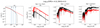 |
Fig. 5. Top-light IMF case (log10(SFR) = −4; [M/H] = 0). Same labels as in Fig. 4. |
| In the text | |
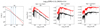 |
Fig. 6. Top-heavy IMF case (log10(SFR) = 2; [M/H] = −0.4). Same labels as in Fig. 4. |
| In the text | |
|
Fig. 7. Index information of NaD. Each index panel contains four vertical sub-panels. The first top panel represents the index value (in black based on canonical IMF and with a colour palette based on gwIMF for different SFRs) for a solar metallicity of [M/H] = 0. Similarly, the bottom panels represent the difference between the index based on gwIMF with different SFRs and the one based on the canonical IMF. From the second to the fourth panel, each one represents different metallicities (in order [M/H] = −0.4, [M/H] = 0, [M/H] = 0.22), signalling in each case a representative observational error obtained for a signal-to-noise ratio of S/N = 50 (dashed grey line) and S/N = 100 (dotted grey line). |
| In the text | |
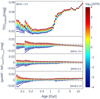 |
Fig. 8. Index information of TiO2(sdss). Labels are the same as in Fig. 7. |
| In the text | |
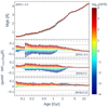 |
Fig. 9. Index information of Mgb. Labels are the same as in Fig. 7. |
| In the text | |
 |
Fig. 10. Index information of ⟨Fe⟩. Labels are the same as in Fig. 7. |
| In the text | |
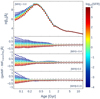 |
Fig. 11. Index information of Hβo. Labels are the same as in Fig. 7. |
| In the text | |
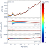 |
Fig. A.1. IMF indicator: aTiO. Same labels as in Fig. 7. |
| In the text | |
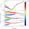 |
Fig. A.2. IMF indicator: bTiO. Same labels as in Fig. 7. |
| In the text | |
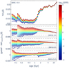 |
Fig. A.3. IMF indicator: TiO1. Same labels as in Fig. 7. |
| In the text | |
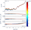 |
Fig. A.4. IMF indicator: CaH1. Same labels as in Fig. 7. |
| In the text | |
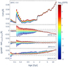 |
Fig. A.5. IMF indicator: CaH2. Same labels as in Fig. 7. |
| In the text | |
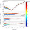 |
Fig. A.6. IMF indicator: Mg4780. Same labels as in Fig. 7. |
| In the text | |
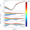 |
Fig. A.7. Abundance indicator: CN2. Same labels as in Fig. 7. |
| In the text | |
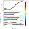 |
Fig. A.8. Abundance indicator: C24668. Same labels as in Fig. 7. |
| In the text | |
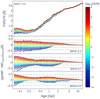 |
Fig. A.9. Abundance indicator: Fe5270. Same labels as in Fig. 7. |
| In the text | |
|
Fig. A.10. Abundance indicator: Fe5335. Same labels as in Fig. 7. |
| In the text | |
|
Fig. A.11. Age indicator: Hβ. Same labels as in Fig. 7. |
| In the text | |
|
Fig. A.12. Age indicator: HδF. Same labels as in Fig. 7. |
| In the text | |
|
Fig. A.13. Age indicator: Hγσ130. Same labels as in Fig. 7. |
| In the text | |
Current usage metrics show cumulative count of Article Views (full-text article views including HTML views, PDF and ePub downloads, according to the available data) and Abstracts Views on Vision4Press platform.
Data correspond to usage on the plateform after 2015. The current usage metrics is available 48-96 hours after online publication and is updated daily on week days.
Initial download of the metrics may take a while.