| Issue |
A&A
Volume 702, October 2025
|
|
|---|---|---|
| Article Number | A32 | |
| Number of page(s) | 20 | |
| Section | Planets, planetary systems, and small bodies | |
| DOI | https://doi.org/10.1051/0004-6361/202555614 | |
| Published online | 03 October 2025 | |
TOI-2322: Two transiting rocky planets close to the stellar rotation period and its first harmonic
1
Observatoire de Genève, Département d’Astronomie, Université de Genève,
Chemin Pegasi 51b,
1290
Versoix,
Switzerland
2
Instituto de Astrofísica de Canarias, c/ Vía Láctea s/n,
38205
La Laguna, Tenerife,
Spain
3
Departamento de Astrofísica, Universidad de La Laguna,
38206
La Laguna, Tenerife,
Spain
4
Department of Physics, University of Oxford,
Oxford
OX1 3RH,
UK
5
Instituto de Astrofísica e Ciências do Espaço, CAUP, Universidade do Porto, Rua das Estrelas,
4150-762
Porto,
Portugal
6
Departamento de Física e Astronomia, Faculdade de Ciências, Universidade do Porto, Rua do Campo Alegre,
4169-007
Porto,
Portugal
7
Institut d’Estudis Espacials de Catalunya (IEEC), Edifici RDIT, Campus UPC,
08860
Castelldefels (Barcelona),
Spain
8
Institut de Ciències de l’Espai (ICE, CSIC), Campus UAB, c/ de Can Magrans s/n,
08193
Cerdanyola del Vallès, Barcelona,
Spain
9
Physics Institute, University of Bern,
Gesellsschaftstrasse 6,
3012
Bern,
Switzerland
10
Center for Space and Habitability, University of Bern,
Gesellsschaftstrasse 6,
3012
Bern,
Switzerland
11
Centro de Astrobiología, CSIC-INTA,
Camino Bajo del Castillo s/n,
28692
Villanueva de la Cañada, Madrid,
Spain
12
Center for Astrophysics | Harvard & Smithsonian,
60 Garden Street,
Cambridge,
MA
02138,
USA
13
INAF – Osservatorio Astronomico di Trieste,
via G. B. Tiepolo 11,
34143
Trieste,
Italy
14
IFPU–Institute for Fundamental Physics of the Universe,
via Beirut 2,
34151
Trieste,
Italy
15
INAF – Osservatorio Astrofisico di Torino,
Via Osservatorio 20,
10025
Pino Torinese,
Italy
16
Department of Physics and Astronomy, University of New Mexico,
210 Yale Boulevard,
Albuquerque,
NM
87131,
USA
17
European Southern Observatory, Av. Alonso de Cordova,
3107 Vitacura,
Santiago de Chile,
Chile
18
Kavli Institute for Astrophysics and Space Research, Massachusetts Institute of Technology,
70 Vassar St,
Cambridge,
MA
02139,
USA
19
Centro de Astrofísica da Universidade do Porto, Rua das Estrelas,
4150-762
Porto,
Portugal
20
INAF – Osservatorio Astronomico di Palermo,
Piazza del Parlamento 1,
90134
Palermo,
Italy
21
Instituto de Astrofísica e Ciências do Espaço, Faculdade de Ciências da Universidade de Lisboa,
1749-016
Lisboa,
Portugal
22
Hamburger Sternwarte,
Gojenbergsweg 112,
21029
Hamburg,
Germany
23
Subaru Telescope, National Astronomical Observatory of Japan (NAOJ),
650 N Aohoku Place,
Hilo,
HI
96720,
USA
24
SETI Institute,
Mountain View, CA 94043, USA/NASA Ames Research Center,
Moffett Field,
CA
94035,
USA
25
Department of Physics, Engineering and Astronomy, Stephen F. Austin State University,
1936 North St,
Nacogdoches,
TX
75962,
USA
★ Corresponding author: This email address is being protected from spambots. You need JavaScript enabled to view it.
Received:
21
May
2025
Accepted:
25
August
2025
Abstract
Context. Active regions on the stellar surface can induce quasi-periodic radial velocity (RV) variations that can mimic planets and mask true planetary signals. These spurious signals can be problematic for RV surveys such as those carried out by the ESPRESSO consortium.
Aims. Using ESPRESSO and HARPS RVs and activity indicators, we aim to confirm and characterise two candidate transiting planets from TESS orbiting a K4 star with strong activity signals.
Methods. From the ESPRESSO FWHM, TESS photometry, and ASAS-SN photometry, we measure a stellar rotation period of 21.28 ± 0.08 d. We jointly model the TESS photometry, ESPRESSO and HARPS RVs, and activity indicators, applying a multivariate Gaussian process (GP) framework to the spectroscopic data.
Results. We are able to disentangle the planetary and activity components, finding that TOI-2322 b has a 11.307170−0.000079+0.000085 d period, close to the first harmonic of the rotation period, a ≤2.03 M⊕ mass upper limit and a 0.994−0.059+0.057 R⊕ radius. TOI-2322 c orbits close to the stellar rotation period, with a 20.225528−0.000044+0.000039 d period; it has a 18.10−5.36+4.34 M⊕ mass and a 1.874−0.057+0.066 R⊕ radius.
Conclusions. The multivariate GP framework is crucial to separating the stellar and planetary signals, significantly outperforming a one-dimensional GP. Likewise, the transit data is fundamental to constraining the periods and epochs, enabling the retrieval of the planetary signals in the RVs. The internal structure of TOI-2322 c is very similar to that of Earth, making it one of the most massive planets with an Earth-like composition known.
Key words: techniques: photometric / techniques: radial velocities / planets and satellites: composition / planets and satellites: detection / stars: individual: TOI-2322 / stars: rotation
© The Authors 2025
 Open Access article, published by EDP Sciences, under the terms of the Creative Commons Attribution License (https://creativecommons.org/licenses/by/4.0), which permits unrestricted use, distribution, and reproduction in any medium, provided the original work is properly cited.
This article is published in open access under the Subscribe to Open model. This email address is being protected from spambots. You need JavaScript enabled to view it. to support open access publication.
1 Introduction
From the start of radial velocity (RV) exoplanet-hunting surveys, it was clear that stellar activity would pose an obstacle to their endeavours (e.g. Saar & Donahue 1997; Santos et al. 2000). Different stellar phenomena such as oscillations, granulation, magnetic activity, and magnetic cycles induce spurious signals on a range of timescales from minutes to years (see Dumusque et al. 2014; Dumusque 2018 and references therein). Particularly problematic to the detection of exoplanets are active regions – dark spots and bright faculae – generated by magnetic activity on the stellar surface. These distort stellar line profiles, creating spurious quasi-periodic RV signals that match the stellar rotation period, as the active regions rotate into and out of view, but also evolve over time (e.g. Saar & Donahue 1997; Lagrange et al. 2010; Lovis et al. 2011). Persistent active regions can mimic planetary signals, as shown by numerous disproven ‘planets’ from Queloz et al. (2001), the first such case, to systems such as Gl 581 (Forveille et al. 2011; Baluev 2013) or Barnard’s star (Lubin et al. 2021; Artigau et al. 2022) where quasi-periodic activity signals persisted for years.
In order to correctly model planets around these active stars, this stellar activity needs to be accounted for. To do this, Gaussian processes (GPs, Haywood et al. 2014; Rajpaul et al. 2015) have become the typically adopted framework. To constrain the GPs, knowledge of the stellar activity is necessary. This information can be provided by spectroscopic stellar activity indicators. Broadly speaking, these consist of two types: the measurement of specific activity-sensitive stellar lines, such as the Hα line (Cincunegui et al. 2007; Bonfils et al. 2007) or the Ca II H and K lines (Vaughan et al. 1978; Noyes et al. 1984); or the measurement of changes in the shape of the cross-correlation function (CCF) used to measure the RVs (Baranne et al. 1996; Queloz et al. 2001). Persistent active regions on the stellar surface will imprint quasi-periodic variability on these indicators at the stellar rotation period and its harmonics.
In this paper, we present the TOI-2322 system, consisting of a K4 star with clear activity signals and two transiting planets orbiting it close to the rotation period and its first harmonic respectively. The planets were first identified as candidates by the Transiting Exoplanet Survey Satellite (TESS) NASA mission (Ricker et al. 2015). We confirm and characterise these planets using RVs and activity indicators from the Echelle SPectrograph for Rocky Exoplanets and Stable Spectroscopic Observations (ESPRESSO, Pepe et al. 2013, 2021). Located at ESO’s Very Large Telescope (VLT), Paranal, Chile, ESPRESSO reaches an RV precision of better than 25 cm s−1 during a single night. One of the goals of the ESPRESSO Guaranteed Time Observations (GTO, Pepe et al. 2021) is the follow-up of small planet candidates from TESS and Kepler, for which ESPRESSO’s exquisite RV precision is vital. We also incorporate RVs and activity indicators from the High Accuracy Radial velocity Planet Searcher spectrograph (HARPS, Mayor et al. 2003), which is located on the 3.6 m telescope at La Silla Observatory, Chile, to increase the temporal baseline and improve the sampling.
The paper is structured as follows: we describe the data in Section 2. Section 3 presents the stellar characterisation, and Section 4 the system modelling. We discuss our results in Section 5 and conclude in Section 6.
2 Observations
2.1 TESS photometry
TOI-2322 is in the southern TESS continuous viewing zone. It was observed by TESS in sectors 1–3 and 5–13 of the prime mission, from 25 July 2018 to 14 October 2018 and 15 November 2018 to 17 July 2019; sectors 27–33 and 35–39 of the first extended mission, from 5 July 2020 to 13 January 2021 and 2 February 2021 to 24 June 2021; and sectors 61–63 and 65–69 of the second extended mission, from 18 January 2023 to 6 April 2023 and 4 May 2023 to 20 September 2023. Camera 4 was used throughout. CCD 1 was used for sectors 35–37 and 61–63; CCD 2 for sectors 11–13, 27, 38–39, and 65–67; CCD 3 for sectors 1–3, 28–30, and 68–69; and CCD 4 for sectors 5–7 and 31–33. During the prime mission, it was observed only in the full frame images at 30 minute cadence. For the extended missions, it was observed at 2-minute cadence.
The TESS photometry was processed by the TESS Science Processing Operations Center (SPOC, Jenkins et al. 2016) at NASA Ames Research Center. Two potential transit signals at ~20.2 d and ~11.3 d were identified by the TESS Quick Look Pipeline (Kunimoto et al. 2021), and designated as TESS Objects of Interest TOI-2322.01 and TOI-2322.02 by the TESS Science Office (Guerrero et al. 2021) on 7 October 2020 and 12 August 2021, respectively. We highlight that the longer-period signal was identified first, due to its greater depth, and is thus numbered first. For our analysis, we use both the SPOC Simple Aperture Photometry (SAP) light curves (Twicken et al. 2010; Morris et al. 2020) and the SPOC Presearch Data Conditioning Simple Aperture Photometry (PDC-SAP) light curves (Stumpe et al. 2012, 2014; Smith et al. 2012). These are only available for the 2-minute cadence data from the extended missions, which is shown in Fig. A.1. Given the wealth of 2-minute cadence data, we do not include the prime mission lower-cadence photometry. We also note that the transits are of relatively short duration, spanning less than three hours from ingress to egress; at 30-minute cadence, there are only four to six points within each transit, making it difficult to correctly fit for the transit shape.
TESS has a large pixel size of 21″ per pixel, meaning the photometry can be contaminated by nearby stars. We used the tpfplotter package1 (Aller et al. 2020) and the TESS-cont algorithm2 (Castro-González et al. 2024) to search for potential contaminants in the TESS aperture used for TOI-2322. Nearby stars with a magnitude contrast down to 9 could mimic the smaller of the transit depths, that of TOI-2322.02 (Lillo-Box et al. 2014). Figure 1 shows the TESS target pixel file and SPOC pipeline aperture for sector 27. Accounting for the relative location of the nearby sources with respect to the SPOC aperture and the TESS pixel response functions (PRFs), TESS-cont finds that a 6.5% eclipse in the most contaminating source (TIC 300812728; Star#8 in Fig. 1) could generate the transit signal TOI-2322.02. A similar conclusion is reached for TIC 300812734 (Star#7) and TIC 764823031 (Star#2), with 29.8% and 33.3% eclipses potentially generating the observed signal. We note that we discard this possibility through follow-up transit observations (see Sect. 2.2), and that the PDCSAP data already account for flux dilution, so no additional corrections were necessary. The target pixel files for the remaining sectors with PDCSAP 2-minute cadence data are shown in Figs. B.1 and B.2.
As a complementary measurement to the ground-based follow-up, we obtain the difference-image centroid measurement from the SPOC analysis. The Data Validation module of the SPOC pipeline (Twicken et al. 2018) measures the location of the TOI-2322.01 transits to be 2.5 ± 3.1″ from TOI-2322, i.e. consistent with the presumed host. This measurement also excludes the surrounding stars as sources of the transits.
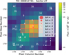 |
Fig. 1 TESS target pixel file for TOI-2322 for sector 27. The target star is labelled as 1 and marked by a white cross. All sources from the Gaia DR3 catalogue down to a magnitude contrast of 9 are shown as red circles, with the size proportional to the contrast. The SPOC pipeline aperture is overplotted in shaded red squares. |
2.2 Ground-based photometry
As the TESS pixel size is large and nearby stars can thus contaminate the photometry, follow-up ground-based photometry is used to vet the nearby stars as potential background eclipsing binaries (EBs), which can cause false-positive exoplanet detections (Lillo-Box et al. 2012). We observed a full transit window of TOI-2322.01 continuously for 145 minutes in Sloan i′ band on UTC 2022 November 23 from the Las Cumbres Observatory Global Telescope (LCOGT) (Brown et al. 2013) 1 m network node at Siding Spring Observatory near Coonabarabran, Australia (SSO). The 1 m telescope is equipped with a 4096 × 4096 SINISTRO camera having an image scale of ![Mathematical equation: $\[0^{\prime\prime}_\cdot389\]$](/articles/aa/full_html/2025/10/aa55614-25/aa55614-25-eq6.png) per pixel, resulting in a 26′ × 26′ field of view. The images were calibrated by the standard LCOGT BANZAI pipeline (McCully et al. 2018) and differential photometric data were extracted using AstroImageJ (Collins et al. 2017). We used the TESS Transit Finder, which is a customised version of the Tapir software package (Jensen 2013), to schedule our transit observations.
per pixel, resulting in a 26′ × 26′ field of view. The images were calibrated by the standard LCOGT BANZAI pipeline (McCully et al. 2018) and differential photometric data were extracted using AstroImageJ (Collins et al. 2017). We used the TESS Transit Finder, which is a customised version of the Tapir software package (Jensen 2013), to schedule our transit observations.
The TOI-2322.01 SPOC pipeline transit depth of 460 ppm is generally too shallow to reliably detect with ground-based observations, so we instead checked for possible nearby eclipsing binaries (NEBs) that could be contaminating the TESS photometric aperture and causing the TESS detection. To account for possible contamination from the wings of neighbouring star PSFs, we searched for NEBs out to ![Mathematical equation: $\[2^\prime_\cdot5\]$](/articles/aa/full_html/2025/10/aa55614-25/aa55614-25-eq7.png) from TOI-2322. If fully blended in the SPOC aperture, a neighbouring star that is fainter than the target star by 8.4 magnitudes in TESS-band could produce the SPOC-reported flux deficit at mid-transit (assuming a 100% eclipse). To account for possible TESS magnitude uncertainties and possible delta-magnitude differences between TESS-band and Sloan i′ band, we included an extra 0.5 magnitudes fainter (down to TESS-band magnitude 18.9). We calculated the RMS of each of the 62 nearby star light curves (binned in 10 minute bins) that meet our search criteria and find that the values are smaller by at least a factor of 5 compared to the required NEB depth in each respective star. We then visually inspected each neighbouring star’s light curve to ensure that there is no obvious eclipse-like signal. Our analysis ruled out an NEB blend as the cause of the SPOC pipeline TOI-2322.01 detection in the TESS data. All LCOGT light curve data are available on the EXOFOP-TESS website3.
from TOI-2322. If fully blended in the SPOC aperture, a neighbouring star that is fainter than the target star by 8.4 magnitudes in TESS-band could produce the SPOC-reported flux deficit at mid-transit (assuming a 100% eclipse). To account for possible TESS magnitude uncertainties and possible delta-magnitude differences between TESS-band and Sloan i′ band, we included an extra 0.5 magnitudes fainter (down to TESS-band magnitude 18.9). We calculated the RMS of each of the 62 nearby star light curves (binned in 10 minute bins) that meet our search criteria and find that the values are smaller by at least a factor of 5 compared to the required NEB depth in each respective star. We then visually inspected each neighbouring star’s light curve to ensure that there is no obvious eclipse-like signal. Our analysis ruled out an NEB blend as the cause of the SPOC pipeline TOI-2322.01 detection in the TESS data. All LCOGT light curve data are available on the EXOFOP-TESS website3.
2.3 ESPRESSO radial velocities
TOI-2322 was observed by the ESPRESSO GTO 33 times between 13 November 2022 and 26 March 2023, after the 2019 fibre link replacement (Pepe et al. 2021), under programme IDs 110.24CD.002, 110.24CD.003, and 110.24CD.009 (P.I. F. Pepe). The observations were done with an exposure time of 900 s, save one observation on 28 November 2022 with an increased exposure time of 1200 s due to poor weather conditions. The spectra have a median S/N of 63 at 550 nm. They were processed with the data reduction software (DRS, Pepe et al. 2021) v.3.2.5, in which the RVs are obtained through the CCF method (Baranne et al. 1996). The K6 mask was used to obtain the CCFs. The resulting RVs have a median error of 1.2 m/s.
In addition to RVs, the DRS also computes several activity indicators. Three of these are measured from the CCF: the full width at half maximum (FWHM), contrast, and bisector inverse slope (BIS, Queloz et al. 2001). Others measure chromospheric emission in the cores of specific lines: the Mount-Wilson S-index (SMW, Vaughan et al. 1978) and ![Mathematical equation: $\[\log~ R_{\mathrm{hk}}^{\prime}\]$](/articles/aa/full_html/2025/10/aa55614-25/aa55614-25-eq8.png) (Noyes et al. 1984), for the Ca II H and K lines; the Hα index (Cincunegui et al. 2007; Bonfils et al. 2007), for the Hα line; the Na index (Díaz et al. 2007), for the Na I D1 and D2 lines.
(Noyes et al. 1984), for the Ca II H and K lines; the Hα index (Cincunegui et al. 2007; Bonfils et al. 2007), for the Hα line; the Na index (Díaz et al. 2007), for the Na I D1 and D2 lines.
We downloaded the RVs and activity indicators from the Data & Analysis Center for Exoplanets (DACE) platform4. The RVs are shown in Fig. 6. The generalised Lomb-Scargle (GLS, Zechmeister & Kürster 2009) periodograms of the ESPRESSO RVs and activity indicators are shown in Fig. C.1.
2.4 HARPS radial velocities
TOI-2322 was observed with HARPS 19 times between 8 October 2022 and 16 January 2023, under programme ID 110.242T. 001 (P.I. R. Rebolo). The observations were done with an exposure time of 2700 s. The spectra have a median S/N of 52 at 550 nm. They were processed with a HARPS-adapted version of the ESPRESSO DRS v.3.2.5. As with ESPRESSO, the K6 mask was used to obtain the CCFs. The RVs have a median error of 1.8 m/s.
We again downloaded the RVs and activity indicators from the DACE platform. They are listed in Appendix C, and the RVs are shown in Fig. 6. The GLS periodograms of the HARPS RVs and activity indicators are shown in Fig. C.2.
We show the GLS periodograms of the joint ESPRESSO and HARPs RVs and activity indicators in Fig. 2. To compensate for any potential offset between the two instruments, we have subtracted the medians from each individual time-series prior to generating the periodograms. Significant signals appear close to the ~20 d period of TOI-2322.01 in both the RVs and all activity indicators save the Na index. The Na index likewise does not show significant periodic signals in the individual instruments; this contrasts with the RVs and other activity indicators, which generally show clear signals in the individual HARPS and ESPRESSO datasets (see Figs. C.2 and C.1), although in the smaller HARPS dataset they do not reach as high significance as for ESPRESSO. In general, the Na index is a better activity tracer for M-dwarfs (e.g. Gomes da Silva et al. 2011), and has been seen to be a poor tracer for K-dwarfs (e.g. Barragán et al. 2023). With a B − V = 1.14, it is also close to the B − V = 1.1 threshold below which Díaz et al. (2007) found no clear correlation with activity. There are also smaller tentative peaks close to the ~11 d period of TOI-2322.02 in several activity indicators.
2.5 High-contrast imaging
In addition to ground-based photometry, high-contrast imaging is valuable to vet stars hosting close companions. As well as false positives from close EBs, flux from any close additional source(s) can lead to an underestimated planetary radius if not accounted for in the transit model (Ciardi et al. 2015; Furlan & Howell 2017; Matson et al. 2018; Castro-González et al. 2022). TOI-2322 was observed with optical speckle imaging by the SOAR TESS survey (Ziegler et al. 2020) using the high-resolution camera (HRCam) imager on the 4.1-m Southern Astrophysical Research (SOAR) telescope at Cerro Pachón, Chile (Tokovinin 2018) on 31 October 2020, with no nearby sources detected within 3″. The contrast curve and speckle auto-correlation function are shown in Fig. 3.
3 Stellar parameters
3.1 Atmospheric and physical parameters
The stellar parameters for TOI-2322 are listed in Table 1. We used the Gaia Data Release 3 (Gaia Collaboration 2016, 2023) for its stellar coordinates, proper motions, and parallaxes. We further characterised TOI-2322 using the co-added ESPRESSO spectra, obtaining the atmospheric parameters via spectral synthesis with the STEPARSYN code5 (Tabernero et al. 2022). STEPARSYN provides the effective temperature, Teff, metallicity, [Fe/H], surface gravity, log g, and broadening parameter, vbroad, which accounts for both the macroturbulence, ζ, and the projected rotational velocity, v sin i. We performed an independent validation with the combined ARES+MOOG approach of Sousa (2014). The resulting parameters of Teff = 4499 ± 126 K, [Fe/H] = −0.14 ± 0.05, and log g = 4.56 ± 0.08 are compatible with those derived by STEPARSYN.
To determine the physical parameters of the star, we followed the procedure of Brahm et al. (2019), in which the broadband photometric measurements (converted to absolute magnitudes via the Gaia DR3 (Gaia Collaboration 2016, 2023) parallax) are compared with the stellar evolutionary models of Bressan et al. (2012). We used the STEPARSYN Teff and [Fe/H] as input values, taking the sum of the internal and systematic errors in quadrature. From this method we obtained the mass, radius, bolometric luminosity, and stellar age. We also obtain an independent estimation of log g = 4.64 ± 0.01, consistent with the spectroscopic measurement within the systematic error bar.
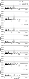 |
Fig. 2 GLS periodograms of the combined ESPRESSO and HARPS RVs (top) and activity indicators (second to bottom: CCF FWHM, CCF contrast, CCF bisector, Hα, |
![Mathematical equation: $\[\log~ \mathrm{R}_{\mathrm{HK}}^{\prime}\]$](/articles/aa/full_html/2025/10/aa55614-25/aa55614-25-eq9.png)
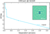 |
Fig. 3 Contrast curve and speckle auto-correlation function from the HRCam at SOAR for TOI-2322. The cyan points and solid line indicate the 5σ contrast curve; the inset shows the speckle auto-correlation function. No nearby sources are detected. |
3.2 Stellar rotation
TOI-2322 shows strong evidence of stellar activity, with highly significant peaks at a ~21 d period in most of the spectral activity indicators (Fig. 2). The TESS PDCSAP light curves, which we use for our transit fits, likewise show strong variability (Fig. A.1). We computed the GLS periodogram of the PDC-SAP light curves, which is shown in Fig. 4. While the highest power is obtained for a period of ~10 d, there are also peaks at the ~21 d period where all the spectral activity indicators peak. Since the PDC systematic error correction algorithm is known to distort astrophysical signals with timescales longer than about half a TESS sector (~14 days)6, we derive a more robust estimate of the stellar rotation by computing the GLS periodogram of the SPOC Simple Aperture Photometry (SAP) light curves. The light curves are shown in Fig. A.2 and the GLS periodogram in Fig. 4. The highest power is seen at ~21 d.
We also obtained ground-based g-band photometry from the All-Sky Automated Survey for Supernovae (ASAS-SN, Shappee et al. 2014; Kochanek et al. 2017), spanning a 7-year interval from 6 October 2017 to 5 October 2024, overlapping the TESS and ESPRESSO observations. The light curve and periodogram are shown in Fig. 5. The strongest periodogram peaks are at ~1111 d ≈ 3 yr and ~21 d, with a smaller peak at ~10 d.
Taking into account all the data, we conclude the most likely stellar rotation period is Prot ~ 21 d. The ~10 d peaks in the TESS PDSCAP periodogram would then correspond to the Prot/2 harmonic. To determine a final rotation period value, we fit Gaussians to the ~21 d peaks in the FWHM and ASAS-SN photometry periodograms, taking the mean and standard deviation as the Prot value and error. For the FWHM, we obtain Prot = 21.3 ± 1.4 d. For the ASAS-SN photometry, we obtain Prot = 21.28 ± 0.08 d; we adopt this last, more precise value as our rotation period.
Stellar parameters for TOI-2322.
4 Data analysis
Modelling a planetary system with significant stellar activity is complex, particularly when the stellar rotation period is close to a planet period. Gaussian process regression has become a standard way to deal with quasi-periodic stellar activity signals (see e.g. Haywood et al. 2014; Rajpaul et al. 2015). In this paper, we test two approaches: One incorporating a single GP with the juliet7 software (Espinoza et al. 2019), detailed in Section 4.1, and a more sophisticated multivariate GP regression with the pyaneti8 software (Barragán et al. 2019; Barragán et al. 2022), detailed in Section 4.2. We also test different GP kernels (Section 4.3) and RV extraction methods (Section 4.4), to ensure the robustness of our results.
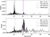 |
Fig. 4 GLS periodogram of the TESS PDCSAP light curves (top) and SAP light curves (bottom). The vertical green and purple lines mark the periods of TOI-2322.02 and TOI-2322.01, respectively; the vertical red line marks the period of the highest power seen in the FWHM periodogram. The dotted horizontal grey line indicates the 0.1% FAP level. |
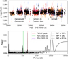 |
Fig. 5 Light curve (top, separated by camera in colours, and 1-day binned data in black) and GLS periodogram (bottom) of the ASAS-SN g-band photometry. The vertical green and purple lines indicate the periods of TOI-2322.02 and TOI-2322.01, respectively, while the vertical red line indicates the period of highest power seen in the FWHM periodogram. The dotted, dashed, and solid horizontal grey lines indicate the 10%, 1%, and 0.1% FAP levels, respectively. |
4.1 Preliminary joint fit with juliet
We first fitted the ESPRESSO RVs and TESS PDCSAP photometry simultaneously using the juliet software. We tested four models: a single transiting planet on a circular orbit at the period of TOI-2322.02 (model in), a single transiting planet on a circular orbit at the period of TOI-2322.01 (model out), two transiting planets on circular orbits (model 2c), and two transiting planets on free-eccentricity orbits (model 2e). Given the strong stellar activity apparent in both the spectral activity indicators and the photometry, we used GPs to model it in both the RVs and photometry.
Given the large quantities of TESS data, we used a two-step process where we first fit a GP to the out-of-transit data in each sector, then apply it to the in-transit data and use only this detrended in-transit data in the full fits. For this, we first masked the in-transit data, with a 5h padding of the transit window. We then fitted the out-of-transit data using the (approximate) Matérn 3/2 kernel, as implemented in celerite, with broad log-uniform priors of 𝒥(1 × 10⁻⁶, 1 × 10⁶) for the GP amplitude, σGP,sector, and 𝒥(1 × 10⁻³, 1 × 10³) for the GP length-scale, ρGP,sector. We also fitted the instrumental parameters for each sector, taking broad priors of 𝒩(0.0, 0.1) for the flux offset, mflux,sector and 𝒥(0.1, 1000) for the jitter, σw,sector, and setting the dilution factor, mdilution,sector, to 1. The priors and posteriors for these fits are listed in Tables D.3 and D.4. Finally, we use these GPs to detrend the in-transit data, which was used in the full fit. This detrended in-transit data was also used for the pyaneti analysis.
We present the details and full results of this analysis in Appendix D. Here, we highlight that the 2c model is favoured by likelihood comparison, and that this single-GP approach is not sufficient to characterise the system, as we do not reach a 3σ semi-amplitude measurement for either planet. With the 2c model, for TOI-2322.02 we find a period of ![Mathematical equation: $\[11.30727_{-0.00013}^{+0.00029}\]$](/articles/aa/full_html/2025/10/aa55614-25/aa55614-25-eq16.png) d, a radius of 1.01 ± 0.08 R⊕, and a semi-amplitude of
d, a radius of 1.01 ± 0.08 R⊕, and a semi-amplitude of ![Mathematical equation: $\[2.8_{-1.7}^{+2.3}\]$](/articles/aa/full_html/2025/10/aa55614-25/aa55614-25-eq17.png) m s−1, leading to an upper mass limit of < 26.66 M⊕. For TOI-2322.01 we find a period of
m s−1, leading to an upper mass limit of < 26.66 M⊕. For TOI-2322.01 we find a period of ![Mathematical equation: $\[20.225520_{-0.000041}^{+0.000037}\]$](/articles/aa/full_html/2025/10/aa55614-25/aa55614-25-eq18.png) d, a radius of 1.94 ± 0.13 R⊕, and a semi-amplitude of
d, a radius of 1.94 ± 0.13 R⊕, and a semi-amplitude of ![Mathematical equation: $\[4.90_{-2.94}^{+2.99}\]$](/articles/aa/full_html/2025/10/aa55614-25/aa55614-25-eq19.png) m s−1, giving an upper mass limit of <46.87 M⊕.
m s−1, giving an upper mass limit of <46.87 M⊕.
4.2 Multivariate GP fit with pyaneti
While the juliet fit showed promising results, the uncertainties on the semi-amplitudes, and thus the masses, were large. Therefore, we decided to explore a more sophisticated modelling of the activity signal with pyaneti. pyaneti is an RV and transit modelling software, presented in Barragán et al. (2019), which allows for joint RV and transit fitting, using MCMC sampling to explore the parameter space. Its second version (Barragán et al. 2022) also incorporates multidimensional GP regression, using the framework of Rajpaul et al. (2015).
We simultaneously fitted the same detrended TESS in-transit photometry and ESPRESSO RVs as used in the juliet fits. For this analysis, we also incorporated the HARPS RVs. We tested the same four in, out, 2c, and 2e models. For all the models, we used a multivariate GP on the RVs and activity indicators to constrain the stellar activity impact on the RVs. The framework of Rajpaul et al. (2015) uses two activity indicators: one which depends only on the fractional coverage by active regions, such as ![Mathematical equation: $\[\log~ \mathrm{R}_{\mathrm{HK}}^{\prime}\]$](/articles/aa/full_html/2025/10/aa55614-25/aa55614-25-eq20.png) or FWHM; and one which, like the RV, is also affected by the stellar surface velocity at the active regions, such as BIS. Barragán et al. (2023) explored one-, two-, and three-dimensional GPs in this framework and concluded the three-dimensional GPs provided the best constraints. We thus elected to model the RVs simultaneously with two activity indicators that have the desired properties. Since our
or FWHM; and one which, like the RV, is also affected by the stellar surface velocity at the active regions, such as BIS. Barragán et al. (2023) explored one-, two-, and three-dimensional GPs in this framework and concluded the three-dimensional GPs provided the best constraints. We thus elected to model the RVs simultaneously with two activity indicators that have the desired properties. Since our ![Mathematical equation: $\[\log~ \mathrm{R}_{\mathrm{HK}}^{\prime}\]$](/articles/aa/full_html/2025/10/aa55614-25/aa55614-25-eq21.png) time series shows some outliers and a slightly weaker periodicity at 21 d, we chose to use the FWHM as the first activity indicator. For the second, we examined the correlations between the RVs and each activity indicator. As the BIS shows a strong anti-correlation with the RVs, we selected it as our second activity indicator. We also note these indicators are the same ones that were used in Barragán et al. (2023) to model the active K3 star K2-233. Our GP model is thus expressed as
time series shows some outliers and a slightly weaker periodicity at 21 d, we chose to use the FWHM as the first activity indicator. For the second, we examined the correlations between the RVs and each activity indicator. As the BIS shows a strong anti-correlation with the RVs, we selected it as our second activity indicator. We also note these indicators are the same ones that were used in Barragán et al. (2023) to model the active K3 star K2-233. Our GP model is thus expressed as
![Mathematical equation: $\[\begin{aligned}& R V=A 0_{G P, r v} G(t)+A 1_{G P, r v} \dot{G}(t), \\& F W H M=A 2_{G P, F W H M} G(t), \\& B I S=A 4_{G P, B I S} G(t)+A 5_{G P, B I S} \dot{G}(t),\end{aligned}\]$](/articles/aa/full_html/2025/10/aa55614-25/aa55614-25-eq22.png) (1)
(1)
with G(t) a GP with a quasi-periodic covariance kernel
![Mathematical equation: $\[\gamma^{(G, G)}\left(t, t^{\prime}\right)=\exp \left\{-\frac{\sin ^2\left[\pi\left(t-t^{\prime}\right) / P\right]}{2 \lambda_p^2}-\frac{\left(t-t^{\prime}\right)^2}{2 \lambda_e^2}\right\}.\]$](/articles/aa/full_html/2025/10/aa55614-25/aa55614-25-eq23.png) (2)
(2)
For joint RV and transit fits, pyaneti takes as inputs the following parameters for each planet i: period, Pi, time of midtransit, t0,p, planet-to-star radius ratio, pi, impact parameter, bi, and either eccentricity, ei, and angle of periastron, ωi, or a derived parametrisation such as ![Mathematical equation: $\[\sqrt{e_{i}} ~\sin~ \omega_{\mathrm{i}}, \sqrt{e_{i}} ~\cos~ \omega_{\mathrm{i}}\]$](/articles/aa/full_html/2025/10/aa55614-25/aa55614-25-eq24.png) , which is the parametrisation we adopt. It can fit either ai/R⋆ for each planet, or the stellar density, ρ; we use the latter parametrisation. It also fits an offset, μ, and jitter, σ, for each RV or activity time series, which for this analysis are fitted to the ESPRESSO and HARPS data separately, thus allowing for offsets between the two instruments. Likewise, it fits a jitter, σ, and limb-darkening parameters, q1 and q2, for each transit time series; here we treat all the TESS sectors as a single instrument. The parameters for the quasiperiodic kernel are expressed in slightly different formulations to juliet, such that
, which is the parametrisation we adopt. It can fit either ai/R⋆ for each planet, or the stellar density, ρ; we use the latter parametrisation. It also fits an offset, μ, and jitter, σ, for each RV or activity time series, which for this analysis are fitted to the ESPRESSO and HARPS data separately, thus allowing for offsets between the two instruments. Likewise, it fits a jitter, σ, and limb-darkening parameters, q1 and q2, for each transit time series; here we treat all the TESS sectors as a single instrument. The parameters for the quasiperiodic kernel are expressed in slightly different formulations to juliet, such that ![Mathematical equation: $\[\lambda_{e}=\sqrt{1 / 2 \alpha_{G P}}\]$](/articles/aa/full_html/2025/10/aa55614-25/aa55614-25-eq25.png) and
and ![Mathematical equation: $\[\lambda_{p}=\sqrt{1 / 2 \Gamma_{G P}}\]$](/articles/aa/full_html/2025/10/aa55614-25/aa55614-25-eq26.png) .
.
To set priors on the periods and times of mid-transit, we used the values from the TOI designation, as reported by the EXOFOP-TESS website. We set broad uniform priors on the semi-amplitudes, planet-to-star radius ratios, impact parameters, stellar density, and ![Mathematical equation: $\[\sqrt{e_{i}} ~\sin~ \omega_{\mathrm{i}}, \sqrt{e_{i}} ~\cos~ \omega_{\mathrm{i}}\]$](/articles/aa/full_html/2025/10/aa55614-25/aa55614-25-eq27.png) where applicable. For the RV GP hyper-parameters, we set a uniform prior around the measured stellar rotation period for the period PGP, and broad uniform priors for the length-scale λp,GP and the evolutionary timescale λe,GP (while ensuring this last is longer than PGP). For the amplitudes A0GP,rv − A5GP,BIS, we generally followed the prescriptions of Delisle et al. (2022) to set bounds based on the RMS of the respective data series. Preliminary fits showed positive-negative degeneracies for the A2GP,FWHM and A5GP,BIS components. As the FWHM showed a positive correlation with the RVs, and the corresponding GP component for the RVs A0GP,rv is by convention fixed positive, we additionally set A2GP,FWHM to be positive. Likewise, as the BIS showed a strong negative correlation with the RVs, we set A5GP,BIS to be negative. For the limb-darkening parameters we set broad uniform priors. The remaining instrumental parameters are set internally by pyaneti with broad uniform or log-uniform priors.
where applicable. For the RV GP hyper-parameters, we set a uniform prior around the measured stellar rotation period for the period PGP, and broad uniform priors for the length-scale λp,GP and the evolutionary timescale λe,GP (while ensuring this last is longer than PGP). For the amplitudes A0GP,rv − A5GP,BIS, we generally followed the prescriptions of Delisle et al. (2022) to set bounds based on the RMS of the respective data series. Preliminary fits showed positive-negative degeneracies for the A2GP,FWHM and A5GP,BIS components. As the FWHM showed a positive correlation with the RVs, and the corresponding GP component for the RVs A0GP,rv is by convention fixed positive, we additionally set A2GP,FWHM to be positive. Likewise, as the BIS showed a strong negative correlation with the RVs, we set A5GP,BIS to be negative. For the limb-darkening parameters we set broad uniform priors. The remaining instrumental parameters are set internally by pyaneti with broad uniform or log-uniform priors.
As with the juliet analysis, the two-planet circular model is favoured by likelihood and BIC comparison, with Δ ln ℒ2c–in ≈ 255, Δ ln ℒ2c–out ≈ 62, and Δ ln ℒ2c–2e ≈ 8. The priors and posteriors for all the parameters are listed in Table 2. Figure 6 shows the GP models (and, for the RVs, two-Keplerian model) fitted to the RV, FWHM, and BIS time series. We highlight the clear agreement between the HARPS and ESPRESSO time series. The phase-folded RVs and light curves are shown in Figs. 7 and 8, respectively. The final parameters are consistent with those of the juliet fit, but with tighter constraints. In particular, the semi-amplitude Kc of the outer planet is measured to 3.36σ, significantly better than the 1.67σ measurement obtained with juliet, thus providing a solid detection and mass measurement rather than a mass upper limit. For the inner planet, we continue to not reach a 3σ measurement of Kb, as although the uncertainty decreases by a factor ~3, the best-fit value decreases by a similar factor. The typically reported 3σ upper limit on the mass, however, would lead to an unphysically dense planet, as we will discuss in Section 5. Therefore, we report in Table 2 the computed mass and uncertainties resulting from the best-fit value of Kb. From here onwards, we refer to TOI-2322.02 as TOI-2322 b, and to TOI-2322.01 as TOI-2322 c.
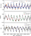 |
Fig. 6 Top: ESPRESSO RVs (blue dots), HARPS RVs (orange diamonds), model components (GP: blue, Keplerian: red), and median model (black) for the pyaneti 2c model. Centre: ESPRESSO (green dots) and HARPS (and red diamonds) FWHM values and joint GP model (black). Bottom: ESPRESSO (purple dots) and HARPS (brown diamonds) BIS values and joint GP model (black). In all panels, solid error bars show the pipeline errors, semi-transparent error bars the added jitter, and dark and light grey regions the 1σ and 2σ confidence intervals. The systemic offsets have been subtracted. |
4.3 Testing different GP kernels
The quasiperiodic GP kernel is a common choice to model stellar activity for various reasons: it is physically motivated, given we expect stellar activity signals to be modulated by the stellar rotation period; it has a low number of hyper-parameters, making it computationally attractive; and it has been shown to reproduce both simulated and real data well (Haywood et al. 2014; Rajpaul et al. 2015; Barragán et al. 2022). However, other kernel choices are possible. To verify the robustness of our results to different kernel choices, we performed additional fits of the detrended TESS photometry and HARPS and ESPRESSO RVs with alternative kernels for the RV GP using the S+LEAF9 software (Delisle et al. 2020, 2022; Hara & Delisle 2025). Specifically, we tested the following four cases: a linear combination of two stochastically driven harmonic oscillator (SHO, Foreman-Mackey et al. 2017) kernels; a Matérn 3/2 exponential periodic (MEP, Delisle et al. 2022) kernel; an exponential-sine periodic (ESP, Delisle et al. 2022) kernel; and an ESP kernel with four defined harmonic components rather than the default two components (ESP-4). The different kernels used and the RV semi-amplitudes obtained for the two planets with each kernel are listed in Table 3. In all cases, the obtained semi-amplitudes are consistent both with the pyaneti analysis and with each other at 1σ, highlighting the robustness of our results. We show the fitted models for each kernel in Appendix E. All the models strongly resemble both each other and the pyaneti model shown in Fig. 6. We highlight as commonalities the large amplitude of the RV GPs, which are much larger than the Keplerian model amplitudes; the sharp peaks of the FWHM model; and the broader, flatter peaks of the BIS model.
Prior and posterior planetary parameter distributions obtained with pyaneti for the 2c model. Top: fitted parameters. Bottom: derived orbital parameters and physical parameters.
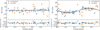 |
Fig. 7 Top: phase-folded ESPRESSO RVs (blue dots), HARPS RVs (orange diamonds), and median Keplerian model (black line) from the pyaneti 2c fit for the inner candidate planet TOI-2322.02 (left) and outer candidate planet TOI-2322.01 (right). The shaded grey regions show the 1σ and 2σ confidence intervals. Bottom: residuals to the fit. |
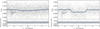 |
Fig. 8 Top: stacked phase-folded PDCSAP TESS data (grey dots), binned TESS data (blue dots), and the median model (black line) from the pyaneti 2c fit, for the inner candidate TOI-2322.02 (left) and outer candidate TOI-2322.01 (right). Bottom: residuals to the fit. |
4.4 Testing different data reductions
While the CCF method for computing radial velocities is a long-enduring field standard, newer techniques based on different principles such as template-matching (Anglada-Escudé & Butler 2012; Astudillo-Defru 2015) and line-by-line (LBL, Dumusque 2018; Artigau et al. 2022) computation have been shown to improve the RV extraction, especially for active stars (e.g. Zhao et al. 2022 and references therein). We first re-extracted the ESPRESSO RVs with the S-BART pipeline (Silva et al. 2022), which uses template matching to extract RV measurements in a semi-Bayesian framework, and tested the juliet 2c model with these RVs. Subsequently, we re-extracted both HARPS and ESPRESSO RVs, FWHM, and BIS using the YARARA pipeline (Cretignier et al. 2021, 2023), which corrects for telluric, stellar, and instrumental effects at the spectral level before extracting LBL RVs, and tested the pyaneti 2c model with these RVs and activity indicators. While in both cases our results were fully compatible with those obtained using the DRS RVs and activity indicators, in neither case did we obtain an improvement on the precision of the fitted semi-amplitudes. This is likely due to the spectra only reaching a moderate S/N, the relatively low number of measurements, and the host star being outside the optimal spectral types for either technique. YARARA, for example, is optimised for sun-like stars and TOI-2322 lies close to the lower edge of its range of validity in Teff. S-BART, meanwhile, shows the most significant gain in RV scatter and median uncertainty for M-dwarfs, while TOI-2322 is a K4 star.
Results from different S+LEAF GP kernels with the pyaneti values for comparison.
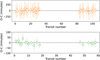 |
Fig. 9 O-C plots for TOI-2322.02 (top) and TOI-2322.01 (bottom). Solid error bars correspond to the 1 − σ error, fainter bars to the 3 − σ error. |
4.5 Impact of including the HARPS data
As the HARPS data have a lower precision, and show more scatter around the best-fit model obtained with the full dataset compared to the ESPRESSO data, we ran a comparison fit using pyaneti with the ESPRESSO data alone. Other than the removal of the HARPS offsets and jitters, all priors are identical to those in Table 2. We find overall larger error bars for the planets’ semi-amplitudes and the GP coefficients, indicating that despite their lower precision the HARPS data are contributing to the fit. We also note that their inclusion extends the temporal baseline covered by approximately a rotation period and a half, as seen in Fig. 6. Since the majority of the ESPRESSO data are clustered in only five rotation periods, this is a substantial increase.
4.6 Search for transit timing variations
Since the periods of the planet candidates are close to the 2:1 resonance, we carried out a search for transit timing variations (TTVs) with juliet. The input parameters for a TTV fit are the expected time of each transit; the stellar density ρ; the planet-to-star radius ratio pi, impact parameter bi, and either eccentricity ei and angle of periastron ωi or a derived parametrisation such as ![Mathematical equation: $\[\sqrt{e_{i}} ~\sin~ \omega_{\mathrm{i}}, \sqrt{e_{i}} ~\cos~ \omega_{\mathrm{i}}\]$](/articles/aa/full_html/2025/10/aa55614-25/aa55614-25-eq86.png) for each planet i; and the dilution factor mdilution,instrument, flux offset mflux,instrument, jitter σw,instrument, and limb-darkening parameters q1,instrument and q2,instrument for each transit instrument. To make the fit computationally feasible, we used the sector-by-sector GP fits to the out-of-transit data described in Appendix D to detrend the in-transit data, then treated it all as coming from a single instrument. We find no strong evidence for TTVs for either planet, as shown in Fig. 9. For TOI-2322 b, the best-fit O-C values have a median amplitude of ~38 minutes with a median error of ~96 minutes, while for TOI-2322 c the best-fit O-C values have a median amplitude of ~10 minutes with a median error of ~10 minutes. We note that TOI-2322 b especially has a small transit depth of ~210 ppm, as can be seen in Fig. 8, so the individual transit fits have high uncertainty, leading to the large errors on the O-C values.
for each planet i; and the dilution factor mdilution,instrument, flux offset mflux,instrument, jitter σw,instrument, and limb-darkening parameters q1,instrument and q2,instrument for each transit instrument. To make the fit computationally feasible, we used the sector-by-sector GP fits to the out-of-transit data described in Appendix D to detrend the in-transit data, then treated it all as coming from a single instrument. We find no strong evidence for TTVs for either planet, as shown in Fig. 9. For TOI-2322 b, the best-fit O-C values have a median amplitude of ~38 minutes with a median error of ~96 minutes, while for TOI-2322 c the best-fit O-C values have a median amplitude of ~10 minutes with a median error of ~10 minutes. We note that TOI-2322 b especially has a small transit depth of ~210 ppm, as can be seen in Fig. 8, so the individual transit fits have high uncertainty, leading to the large errors on the O-C values.
5 Discussion
5.1 Planetary composition
To explore the compositions of the planets of the TOI-2322 system and place them in a population context, we show the planets in Fig. 10 together with the small well-characterised planets from the PlanetS catalogue (Otegi et al. 2020; Parc et al. 2024). The mass and radius derived from the best-fit model for TOI-2322 b place it practically on the 100% Fe model. This may indicate a formation in an extremely volatile-poor environment, or a stripping of volatiles by radiation from the active host star; however, the uncertainties on the mass are very large. Since masses larger than that corresponding to a 100% Fe composition are unphysical, we compute an upper mass limit from the 100% Fe model of Mb ≤ 2.03 M⊕, slightly lower than but fully compatible with the mass derived from the best-fit model. TOI-2322 c, meanwhile, lies close to the 50% Fe, 50% silicates line, and becomes the most massive planet with this composition.
To further characterise the internal structure of TOI-2322 c, we performed interior modelling via the ExoMDN code (Baumeister & Tosi 2023)10. ExoMDN uses mixture density networks to perform interior inference modelling. From the planet’s mass, radius, and equilibrium temperature, the software fits a four-layer model consisting of an iron core, a silicate mantle, a water layer, and a H/He atmosphere. The posterior distributions for the ExoMDN model for TOI-2322 c are shown in Fig. 11. We retrieve a model with very similar layer fractions to the Earth of dCore = ![Mathematical equation: $\[0.75_{-0.19}^{+0.11}\]$](/articles/aa/full_html/2025/10/aa55614-25/aa55614-25-eq87.png) , dMantle =
, dMantle = ![Mathematical equation: $\[0.11_{-0.09}^{+0.19}\]$](/articles/aa/full_html/2025/10/aa55614-25/aa55614-25-eq88.png) , dWater =
, dWater = ![Mathematical equation: $\[0.09_{-0.08}^{+0.13}\]$](/articles/aa/full_html/2025/10/aa55614-25/aa55614-25-eq89.png) , and dGas =
, and dGas = ![Mathematical equation: $\[0.03_{-0.02}^{+0.05}\]$](/articles/aa/full_html/2025/10/aa55614-25/aa55614-25-eq90.png) . For comparison, the fractions retrieved for the Earth are dCore =
. For comparison, the fractions retrieved for the Earth are dCore = ![Mathematical equation: $\[0.69_{-0.09}^{+0.06}\]$](/articles/aa/full_html/2025/10/aa55614-25/aa55614-25-eq91.png) , dMantle =
, dMantle = ![Mathematical equation: $\[0.14_{-0.13}^{+0.20}\]$](/articles/aa/full_html/2025/10/aa55614-25/aa55614-25-eq92.png) , dWater =
, dWater = ![Mathematical equation: $\[0.09_{-0.08}^{+0.12}\]$](/articles/aa/full_html/2025/10/aa55614-25/aa55614-25-eq93.png) , and dGas =
, and dGas = ![Mathematical equation: $\[0.05_{-0.04}^{+0.08}\]$](/articles/aa/full_html/2025/10/aa55614-25/aa55614-25-eq94.png) . We thus characterise TOI-2322 c as one of the most massive planets with an Earth-like composition discovered to date, with a mass of
. We thus characterise TOI-2322 c as one of the most massive planets with an Earth-like composition discovered to date, with a mass of ![Mathematical equation: $\[18.10_{-5.36}^{+4.34}\]$](/articles/aa/full_html/2025/10/aa55614-25/aa55614-25-eq95.png) M⊕.
M⊕.
The closest analogues to TOI-2322 c in mass and composition are Kepler-411 b (Sun et al. 2019) and TOI-1347 b (Rubenzahl et al. 2024). Kepler 411 b is more massive and larger than TOI-2322 c, with a TTV-determined mass of 25.6 ± 2.6 M⊕ and a radius of 2.401 ± 0.053 R⊕. It likely has a larger rocky mantle and smaller iron core, with Sun et al. (2019) estimating a 21 ± 21% iron core mass fraction, compared to a core mass fraction from ExoMDN of ![Mathematical equation: $\[85_{-27}^{+10}\]$](/articles/aa/full_html/2025/10/aa55614-25/aa55614-25-eq96.png) % for TOI-2322 c. TOI-1347 b, meanwhile, is somewhat smaller and less massive than TOI-2322 c; it has an RV-measured mass of 11.1 ± 1.2 M⊕ and a radius of 1.8 ± 0.1 R⊕, leading to a larger core mass fraction of 41 ± 27% which makes it more directly comparable to TOI-2322 c. Both planets have shorter periods than TOI-2322 c, with TOI-1347 b in particular belonging to the ultra-short-period (USP) class, and receive significantly higher insolation fluxes which may have contributed to the stripping of any primordial H/He envelopes. While TOI-2322 c receives much lower insolation, the active host star may have contributed to stripping a primordial envelope, or it may have formed in a gas-poor environment and thus never have accreted an envelope at all.
% for TOI-2322 c. TOI-1347 b, meanwhile, is somewhat smaller and less massive than TOI-2322 c; it has an RV-measured mass of 11.1 ± 1.2 M⊕ and a radius of 1.8 ± 0.1 R⊕, leading to a larger core mass fraction of 41 ± 27% which makes it more directly comparable to TOI-2322 c. Both planets have shorter periods than TOI-2322 c, with TOI-1347 b in particular belonging to the ultra-short-period (USP) class, and receive significantly higher insolation fluxes which may have contributed to the stripping of any primordial H/He envelopes. While TOI-2322 c receives much lower insolation, the active host star may have contributed to stripping a primordial envelope, or it may have formed in a gas-poor environment and thus never have accreted an envelope at all.
5.2 Importance of the transit data to the planet detection
Historically, when faced with signals which are seen at the same period (or harmonics thereof) in both RVs and activity indicators, RV blind surveys have tended to attribute these signals entirely to stellar activity (e.g. Butler et al. 2017; Mignon et al. 2024). However, as the TOI-2322 system evidences, planets can and do exist at similar periods to their host star’s rotation period. In order to explore whether the RV data alone could have conclusively revealed the outer planet, which has the clearest RV signal, we perform a pyaneti fit only on the RVs, FWHM, and BIS for the outer planet alone. The priors are analogous to those listed in Table 2, with the exception of the period Pc and epoch t0,c. Lacking the information from the transit, to set a prior on the period we fit a Gaussian to the highest peak in the joint RV periodogram, which returns a median of 20.7 d and a standard deviation of 1.4 d. We conservatively set the prior for the period as a slightly broader Gaussian of 𝒩(20.7, 2). For t0,c we set an uninformative uniform prior spanning a 22 d range centred on the t0,c value from the transit data, to avoid convergence issues at the edge of the prior.
The resulting fit converges to a significantly shorter and more poorly constrained period of P = ![Mathematical equation: $\[19.82_{-2.29}^{+1.57}\]$](/articles/aa/full_html/2025/10/aa55614-25/aa55614-25-eq97.png) d. The epoch posterior is very broad and spans a large part of the prior space, with error bars of ±6 d. The semi-amplitude of K =
d. The epoch posterior is very broad and spans a large part of the prior space, with error bars of ±6 d. The semi-amplitude of K = ![Mathematical equation: $\[2.95_{-2.02}^{+2.89}\]$](/articles/aa/full_html/2025/10/aa55614-25/aa55614-25-eq98.png) ms−1 barely reaches 1.5σ confidence, and is notably lower than the value obtained in the full fit. In contrast, the A0GP,rv and A1GP,rv coefficients are larger, suggesting that part of the planetary signal is being absorbed by the GP. We also note that the RV residuals show no significant signals at the period of TOI-2322 b (or indeed any period), so from a pure-RV survey this planet would not have been detected, and therefore is not included in this analysis.
ms−1 barely reaches 1.5σ confidence, and is notably lower than the value obtained in the full fit. In contrast, the A0GP,rv and A1GP,rv coefficients are larger, suggesting that part of the planetary signal is being absorbed by the GP. We also note that the RV residuals show no significant signals at the period of TOI-2322 b (or indeed any period), so from a pure-RV survey this planet would not have been detected, and therefore is not included in this analysis.
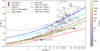 |
Fig. 10 Mass-radius diagram of the well-characterised small planet population (Mp < 40 M⊕, Rp < 4 R⊕, mass error better than 25%, radius error better than 8%) from the PlanetS catalogue (Otegi et al. 2020; Parc et al. 2024) (semi-transparent circles), coloured by insolation. TOI-2322 b and c are shown as a pentagon and a hexagon, respectively. The composition models of Zeng et al. (2019) are shown by the coloured curves. |
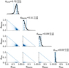 |
Fig. 11 Posterior distributions of the ExoMDN model for TOI-2322 c, showing an internal structure similar to that of the Earth. |
5.3 TOI-2322 as a benchmark system for activity correction
The RV-only analysis demonstrates the vital importance of transiting exoplanet systems like TOI-2322, which are the only systems in which we have as ground truth the existence of both a planet and significant stellar activity at similar periods. With the planet’s period and epoch tightly constrained by the transit data, the RV signal can be properly fitted, enabling a full characterisation of the planet(s). This contrasts with RV-only datasets, where a known stellar activity signal may be masking the presence of a planet at a close period.
The TOI-2322 system is thus an ideal benchmark for testing methods of disentangling these planets from stellar activity. More such planets are likely to emerge as the ongoing extended TESS missions and upcoming transit missions like PLATO begin uncovering more long-period transiting planets with periods in the range of typical stellar rotation periods for main-sequences solar-type stars. Further observations of TOI-2322 would be valuable to extend the observing baseline, enabling the exploration of the time variation of the stellar activity impact on the RVs, refinement of the planetary masses, and the search for additional long-period companions. Simultaneous optical and near-infrared (nIR) spectroscopy would be particularly useful, as stellar activity is wavelength-dependent and has been shown to decrease in the nIR (Carmona et al. 2023). Likewise, co-eval RVs and photometry could enable the simultaneous characterisation of the stellar activity in both datasets (e.g. Hara & Delisle 2025).
6 Conclusions
We have presented the confirmation and characterisation of TOI-2322 b and c, two planets orbiting an active K star. The inner, smaller planet TOI-2322 b has a period slightly above the first harmonic of the rotation period. As we do not reach a 3σ measurement of the semi-amplitude, we use physical considerations to establish an upper mass limit of Mb ≤ 2.03 M⊕, corresponding to the mass of a 100% Fe planet with the ![Mathematical equation: $\[0.994_{-0.059}^{+0.057}\]$](/articles/aa/full_html/2025/10/aa55614-25/aa55614-25-eq99.png) R⊕ radius extracted from the TESS photometry. The outer, larger planet TOI-2322 c has a period slightly below the stellar rotation period, at which significant periodicity is seen in the photometry and spectroscopic activity indicators. It has a mass of
R⊕ radius extracted from the TESS photometry. The outer, larger planet TOI-2322 c has a period slightly below the stellar rotation period, at which significant periodicity is seen in the photometry and spectroscopic activity indicators. It has a mass of ![Mathematical equation: $\[18.10_{-5.36}^{+4.34}\]$](/articles/aa/full_html/2025/10/aa55614-25/aa55614-25-eq100.png) M⊕ and a radius of
M⊕ and a radius of ![Mathematical equation: $\[1.874_{-0.057}^{+0.066}\]$](/articles/aa/full_html/2025/10/aa55614-25/aa55614-25-eq101.png) R⊕, yielding an internal structure very similar to that of the Earth, and so becoming the largest planet known with an Earth-like composition.
R⊕, yielding an internal structure very similar to that of the Earth, and so becoming the largest planet known with an Earth-like composition.
A fitting process involving the photometry, the RVs, and a multivariate GP applied to the RVs and the FWHM and BIS activity indicators was necessary to fully characterise the system, and in particular to separate the stellar activity effects from the planetary signals in the RVs. The TOI-2322 system is an ideal system for testing methods of disentangling planetary and activity signals in RVs. It is also an excellent candidate for follow-up nIR spectroscopy to explore how the interplay between signals of stellar and planetary origin changes across wavelength.
Data availability
RV and activity indicators (Tables C.1, C.2) are available at the CDS via https://cdsarc.cds.unistra.fr/viz-bin/cat/J/A+A/702/A32
Acknowledgements
We thank the referee for their careful reading and helpful comments that have improved this paper. We thank the Swiss National Science Foundation (SNSF) and the Geneva University for their continuous support to our planet low-mass companion search programmes. This work has been carried out within the framework of the National Centre of Competence in Research PlanetS supported by the Swiss National Science Foundation. This publication makes use of The Data & Analysis Center for Exoplanets (DACE), which is a facility based at the University of Geneva (CH) dedicated to extrasolar planets data visualisation, exchange and analysis. DACE is a platform of the Swiss National Centre of Competence in Research (NCCR) PlanetS, federating the Swiss expertise in Exoplanet research. The DACE platform is available at https://dace.unige.ch. This work made use of tpfplotter by J. Lillo-Box (publicly available in www.github.com/jlillo/tpfplotter), which also made use of the python packages astropy, lightkurve, matplotlib and numpy. This work made use of TESS-cont (https://github.com/castro-gzlz/TESS-cont), which also made use of tpfplotter (Aller et al. 2020) and TESS-PRF (Bell & Higgins 2022). This research has made use of the Exoplanet Follow-up Observation Program (ExoFOP; DOI: 10.26134/ExoFOP5) website, which is operated by the California Institute of Technology, under contract with the National Aeronautics and Space Administration under the Exoplanet Exploration Program. Funding for the TESS mission is provided by NASA’s Science Mission Directorate. This paper made use of data collected by the TESS mission and are publicly available from the Mikulski Archive for Space Telescopes (MAST) operated by the Space Telescope Science Institute (STScI). We acknowledge the use of public TESS data from pipelines at the TESS Science Office and at the TESS Science Processing Operations Center. Resources supporting this work were provided by the NASA High-End Computing (HEC) Program through the NASA Advanced Supercomputing (NAS) Division at Ames Research Center for the production of the SPOC data products. This work makes use of observations from the LCOGT network. Part of the LCOGT telescope time was granted by NOIRLab through the Mid-Scale Innovations Program (MSIP). MSIP is funded by NSF. Based on observations made with ESO Telescopes at the La Silla Paranal Observatory under programme IDs 110.24CD.002, 110.24CD.003, and 110.24CD.009. Based on observations carried out at the European Southern Observatory (ESO; La Silla, Chile) using the 3.6m telescope, under ESO programme 110.242T.001. This work has made use of data from the European Space Agency (ESA) mission Gaia (https://www.cosmos.esa.int/gaia), processed by the Gaia Data Processing and Analysis Consortium (DPAC, https://www.cosmos.esa.int/web/gaia/dpac/consortium). Funding for the DPAC has been provided by national institutions, in particular the institutions participating in the Gaia Multilateral Agreement. Co-funded by the European Union (ERC, FIERCE, 101052347). Views and opinions expressed are however those of the author(s) only and do not necessarily reflect those of the European Union or the European Research Council. Neither the European Union nor the granting authority can be held responsible for them. This work was also supported by FCT – Fundação para a Ciência e a Tecnologia through national funds by these grants: UIDB/04434/2020 DOI: 10.54499/UIDB/04434/2020, UIDP/04434/2020 DOI: 10.54499/UIDP/04434/2020, PTDC/FIS-AST/4862/2020, UID/04434/2025. S.G.S. acknowledges the support from FCT through Investigador FCT contract no. CEECIND/00826/2018 and POPH/FSE (EC). S.C.C.B. acknowledges the support from Fundação para a Ciência e Tecnologia (FCT) in the form of work contract through the Scientific Employment Incentive program with reference 2023.06687.CEECIND and DOI 10.54499/2023.06687.CEECIND/CP2839/CT0002. A.C.-G. is funded by the Spanish Ministry of Science through MCIN/AEI/10.13039/501100011033 grant PID2019-107061GB-C61. K.A.C. acknowledges support from the TESS mission via subaward s3449 from MIT. The INAF authors acknowledge financial support of the Italian Ministry of Education, University, and Research with PRIN 201278X4FL and the “Progetti Premiali” funding scheme. X.D. acknowledges the support from the European Research Council (ERC) under the European Union’s Horizon 2020 research and innovation programme (grant agreement SCORE No 851555) and from the Swiss National Science Foundation under the grant SPECTRE (No 200021_215200). J.I.G.H., A.S.M., R.R., and C.A.P. acknowledge financial support from the Spanish Ministry of Science, Innovation and Universities (MICIU) projects PID2020-117493GB-I00 and PID2023-149982NB-I00. J.L.-B. is funded by the Spanish Ministry of Science and Universities (MICIU/AEI/10.13039/501100011033) and NextGenerationEU/PRTR grants PID2019-107061GB-C61 and CNS2023-144309. This work was financed by Portuguese funds through FCT (Fundação para a Ciência e a Tecnologia) in the framework of the project 2022.04048.PTDC (Phi in the Sky, DOI 10.54499/2022.04048.PTDC). C.J.M. also acknowledges FCT and POCH/FSE (EC) support through Investigador FCT Contract 2021.01214.CEECIND/CP1658/CT0001 (DOI 10.54499/2021.01214.CEECIND/CP1658/CT0001). We acknowledge financial support from the Agencia Estatal de Investigación of the Ministerio de Ciencia e Innovación MCIN/AEI/10.13039/501100011033 and the ERDF “A way of making Europe” through project PID2021-125627OB-C32, and from the Centre of Excellence “Severo Ochoa” award to the Instituto de Astrofisica de Canarias. F.P. and C.L. would like to acknowledge the Swiss National Science Foundation (SNSF) for supporting research with ESPRESSO through the SNSF grants nr. 140649, 152721, 166227, 184618 and 215190. The ESPRESSO Instrument Project was partially funded through SNSF’s FLARE Programme for large infrastructures. V.A. acknowledges support from FCT through a work contract funded by the FCT Scientific Employment Stimulus program (reference 2023.06055.CEECIND/CP2839/CT0005, DOI: 10.54499/2023.06055.CEECIND/CP2839/CT0005).
Appendix A TESS light curves
In this appendix we show the sector-by sector TESS SAP and PDCSAP light curves.
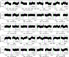 |
Fig. A.1 TESS PDCSAP light curves for TOI-2322. The transits of TOI-2322.02 and TOI-2322.01 are marked by vertical green and purple lines, respectively. The first three rows show the light curves from the first extended mission, while the last two show the light curves from the second extended mission. |
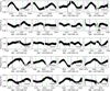 |
Fig. A.2 TESS SAP light curves for TOI-2322. The transits of TOI-2322.02 and TOI-2322.01 are marked by vertical green and purple lines, respectively. The first three rows show the light curves from the first extended mission, while the last two show the light curves from the second extended mission. |
Appendix B TESS pixel file plots
In this appendix we show the TESS pixel file plots for all observed sectors save sector 27, which is shown in Figure 1. Those for the first extended mission are shown in Fig. B.1, and those for the second extended mission in Fig. B.2.
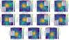 |
Fig. B.1 TESS target pixel files for sectors 28-33 and 35-39, observed during the first extended mission. The target star is labelled as 1 and marked by a white cross in each case. All sources from the Gaia DR3 catalogue down to a magnitude contrast of 9 are shown as red circles, with the size proportional to the contrast. The SPOC pipeline aperture is overplotted in shaded red squares. |
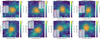 |
Fig. B.2 TESS target pixel files for sectors 61-63 and 65-69, observed during the second extended mission. The target star is labelled as 1 and marked by a white cross in each case. All sources from the Gaia DR3 catalogue down to a magnitude contrast of 9 are shown as red circles, with the size proportional to the contrast. The SPOC pipeline aperture is overplotted in shaded red squares. |
Appendix C Radial velocities and activity indicators
In this appendix we present the ESPRESSO RVs and activity indicators. Figures C.1 and C.2 show the periodograms of the RVs and activity indicators for ESPRESSO and HARPS, respectively.
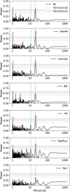 |
Fig. C.1 GLS periodograms of the ESPRESSO RVs (top) and activity indicators (second to bottom: CCF FWHM, CCF contrast, CCF bisector, Hα, |
![Mathematical equation: $\[\log~ \mathrm{R}_{\mathrm{HK}}^{\prime}\]$](/articles/aa/full_html/2025/10/aa55614-25/aa55614-25-eq102.png)
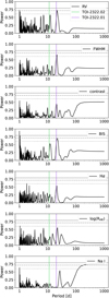 |
Fig. C.2 GLS periodograms of the HARPS RVs (top) and activity indicators (second to bottom: CCF FWHM, CCF contrast, CCF bisector, Hα, |
![Mathematical equation: $\[\log~ \mathrm{R}_{\mathrm{HK}}^{\prime}\]$](/articles/aa/full_html/2025/10/aa55614-25/aa55614-25-eq103.png)
Appendix D juliet fit to the ESPRESSO and TESS data
In this Appendix, we present the detailed juliet fit from Section 4.1. juliet enables the joint fitting of RVs and transit through the radvel package (Fulton et al. 2018) and the batman package (Kreidberg 2015), respectively, and incorporates Gaussian processes (GPs) via the celerite package (Foreman-Mackey et al. 2017). Importance nested sampling, using the dynesty package (Speagle 2020), is employed to explore the parameter space. By default, juliet adopts random walk sampling with 500 live points.
For joint RV and transit fits, juliet takes as parameters the stellar density, ρ; the period, Pi, time of mid-transit, t0,i, RV semi-amplitude, Ki, planet-to-star radius ratio, pi, impact parameter, bi, and either eccentricity, ei, and angle of periastron, ωi, or a derived parametrisation such as ![Mathematical equation: $\[\sqrt{e_{i}} ~\sin~ \omega_{\mathrm{i}}, \sqrt{e_{i}} ~\cos~ \omega_{\mathrm{i}}\]$](/articles/aa/full_html/2025/10/aa55614-25/aa55614-25-eq104.png) for each planet i; the systemic radial velocity, μinstrument, and jitter, σw,instrument, for each RV instrument; and the dilution factor, mdilution,instrument, flux offset, mflux,instrument, jitter, σw,instrument, and limb-darkening parameters, q1,instrument and q2,instrument for each transit instrument. For the limb-darkening parameters, we used the quadratic law parametrisation of Kipping (2013). We take separate dilution factor, flux offset, and jitter for each TESS sector, but joint limb-darkening parameters.
for each planet i; the systemic radial velocity, μinstrument, and jitter, σw,instrument, for each RV instrument; and the dilution factor, mdilution,instrument, flux offset, mflux,instrument, jitter, σw,instrument, and limb-darkening parameters, q1,instrument and q2,instrument for each transit instrument. For the limb-darkening parameters, we used the quadratic law parametrisation of Kipping (2013). We take separate dilution factor, flux offset, and jitter for each TESS sector, but joint limb-darkening parameters.
As noted in Section 4.1, we use GPs to model the stellar activity. For the RVs, we used the quasi-periodic kernel (called exp-sine-squared kernel in juliet) of Haywood et al. (2014), fitted simultaneously with the planet(s). To constrain the priors of this GP, we first fitted a GP to the FWHM activity indicator time series, which has been shown to be a good tracer of stellar activity in ESPRESSO data (Lillo-Box et al. 2020; Lavie et al. 2023; Castro-González et al. 2023), and which shows the highest power at Prot ~ 21 d. The priors and posteriors for this fit are shown in Table D.1. Subsequently, we used the resulting parameters as priors on the radial velocity GP. We use truncated normal priors for σGP,rv, αGP,rv, and ΓGP,rv, centred on the FWHM fit posteriors and taking the larger error bar as the width of the normal prior, truncating at 0 to avoid convergence issues. We also apply a scaling factor to the σGP,FWHM posterior, computed as the ratio of the standard deviation of the two time series, σRV/σFWHM. For ProtGP,FWHM the values are better constrained, so we can use a normal prior on ProtGP,rv.
Prior and posterior planetary parameter distributions obtained with juliet for the FWHM GP model.
For the photometry, meanwhile, we apply a two-step process on a sector-by-sector basis to detrend the in-transit data, which is used in the final fit. The full process is described in Section 4.1.
The Bayesian log-evidence comparison strongly favours a two-planet model over either of the single-planet models, with Δ log Z2c–in ≈ 119 and Δ log Z2c–out ≈ 21. The free-eccentricity two-planet model is not significantly favoured over the circular one, with Δ log Z2e–2c ≈ 0.2. We also tested the same four models without GP detrending, finding that the addition of the GP is favoured in all cases, with Δ log ZGP–noGP ≈ 19 − 24. The priors and posteriors for the favoured 2c model are given in Table D.2. Figure D.1 shows the RVs with the fitted model and phase-folded RVs for both planets, and Figure D.2 shows the phase-folded TESS photometry. Since we do not reach a 3σ measurement of the semi-amplitudes, we compute only upper limits on the planetary masses.
Prior and posterior planetary parameter distributions obtained with juliet for the 2c model. Top: Fitted parameters. Bottom: Derived orbital parameters and physical parameters.
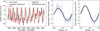 |
Fig. D.1 Left: ESPRESSO RVs (blue dots), model components (GP: red, Keplerian: grey), and median model (black) for the juliet 2c model. The error bars show the RV errors and jitter added in quadrature. The instrumental systemic velocity has been subtracted. The GP fit to the FWHM is also shown (dotted green line) for comparison. Centre and right: phase-folded RVs and median Keplerian model for the inner candidate planet TOI-2322.02 (centre) and outer candidate planet TOI-2322.01 (right). |
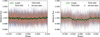 |
Fig. D.2 Stacked phase-folded PDCSAP TESS data with the median model (green line), for the inner candidate TOI-2322.02 (left) and outer candidate TOI-2322.01 (right). The points show the data from the TESS first extended mission (blue), second extended mission (orange), and binned data (black). |
Prior and posterior planetary parameter distributions obtained with juliet for the sector-by-sector detrending of the TESS photometry from the first extended mission.
Prior and posterior planetary parameter distributions obtained with juliet for the sector-by-sector detrending of the TESS photometry from the second extended mission.
Appendix E S+LEAF kernel models
In this Appendix, we show the fitted models using the four S+LEAF kernels described in 4.3.
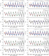 |
Fig. E.1 Fitted models using the S+LEAF kernels. Top to bottom and left to right: 2×SHO kernel, MEP kernel, ESP kernel, and ESP-4 kernel. Within each panel, the subplots are analogous to those in Fig. 6. |
References
- Aller, A., Lillo-Box, J., Jones, D., Miranda, L. F., & Barceló Forteza, S. 2020, A&A, 635, A128 [NASA ADS] [CrossRef] [EDP Sciences] [Google Scholar]
- Anglada-Escudé, G., & Butler, R. P. 2012, ApJS, 200, 15 [Google Scholar]
- Artigau, É., Cadieux, C., Cook, N. J., et al. 2022, AJ, 164, 84 [NASA ADS] [CrossRef] [Google Scholar]
- Astudillo-Defru, N. 2015, PhD thesis, Université Grenoble Alpes [Google Scholar]
- Baluev, R. V. 2013, MNRAS, 429, 2052 [Google Scholar]
- Baranne, A., Queloz, D., Mayor, M., et al. 1996, A&AS, 119, 373 [NASA ADS] [CrossRef] [EDP Sciences] [Google Scholar]
- Barragán, O., Gandolfi, D., & Antoniciello, G. 2019, MNRAS, 482, 1017 [Google Scholar]
- Barragán, O., Aigrain, S., Rajpaul, V. M., & Zicher, N. 2022, MNRAS, 509, 866 [Google Scholar]
- Barragán, O., Gillen, E., Aigrain, S., et al. 2023, MNRAS, 522, 3458 [CrossRef] [Google Scholar]
- Baumeister, P., & Tosi, N. 2023, A&A, 676, A106 [NASA ADS] [CrossRef] [EDP Sciences] [Google Scholar]
- Bell, K. J., & Higgins, M. E. 2022, TESS_PRF: Display the TESS pixel response function, Astrophysics Source Code Library [record ascl:2207.008] [Google Scholar]
- Bonfils, X., Mayor, M., Delfosse, X., et al. 2007, A&A, 474, 293 [NASA ADS] [CrossRef] [EDP Sciences] [Google Scholar]
- Brahm, R., Espinoza, N., Jordán, A., et al. 2019, AJ, 158, 45 [Google Scholar]
- Bressan, A., Marigo, P., Girardi, L., et al. 2012, MNRAS, 427, 127 [NASA ADS] [CrossRef] [Google Scholar]
- Brown, T. M., Baliber, N., Bianco, F. B., et al. 2013, PASP, 125, 1031 [Google Scholar]
- Butler, R. P., Vogt, S. S., Laughlin, G., et al. 2017, AJ, 153, 208 [Google Scholar]
- Carmona, A., Delfosse, X., Bellotti, S., et al. 2023, A&A, 674, A110 [NASA ADS] [CrossRef] [EDP Sciences] [Google Scholar]
- Castro-González, A., Díez Alonso, E., Menéndez Blanco, J., et al. 2022, MNRAS, 509, 1075 [Google Scholar]
- Castro-González, A., Demangeon, O. D. S., Lillo-Box, J., et al. 2023, A&A, 675, A52 [NASA ADS] [CrossRef] [EDP Sciences] [Google Scholar]
- Castro-González, A., Lillo-Box, J., Armstrong, D. J., et al. 2024, A&A, 691, A233 [NASA ADS] [CrossRef] [EDP Sciences] [Google Scholar]
- Ciardi, D. R., Beichman, C. A., Horch, E. P., & Howell, S. B. 2015, ApJ, 805, 16 [NASA ADS] [CrossRef] [Google Scholar]
- Cincunegui, C., Díaz, R. F., & Mauas, P. J. D. 2007, A&A, 469, 309 [NASA ADS] [CrossRef] [EDP Sciences] [Google Scholar]
- Collins, K. A., Kielkopf, J. F., Stassun, K. G., & Hessman, F. V. 2017, AJ, 153, 77 [Google Scholar]
- Cretignier, M., Dumusque, X., Hara, N. C., & Pepe, F. 2021, A&A, 653, A43 [NASA ADS] [CrossRef] [EDP Sciences] [Google Scholar]
- Cretignier, M., Dumusque, X., Aigrain, S., & Pepe, F. 2023, A&A, 678, A2 [NASA ADS] [CrossRef] [EDP Sciences] [Google Scholar]
- Delisle, J. B., Hara, N., & Ségransan, D. 2020, A&A, 638, A95 [EDP Sciences] [Google Scholar]
- Delisle, J. B., Unger, N., Hara, N. C., & Ségransan, D. 2022, A&A, 659, A182 [NASA ADS] [CrossRef] [EDP Sciences] [Google Scholar]
- Díaz, R. F., Cincunegui, C., & Mauas, P. J. D. 2007, MNRAS, 378, 1007 [Google Scholar]
- Dumusque, X. 2018, A&A, 620, A47 [NASA ADS] [CrossRef] [EDP Sciences] [Google Scholar]
- Dumusque, X., Boisse, I., & Santos, N. C. 2014, ApJ, 796, 132 [NASA ADS] [CrossRef] [Google Scholar]
- Espinoza, N., Kossakowski, D., & Brahm, R. 2019, MNRAS, 490, 2262 [Google Scholar]
- Foreman-Mackey, D., Agol, E., Ambikasaran, S., & Angus, R. 2017, AJ, 154, 220 [Google Scholar]
- Forveille, T., Bonfils, X., Delfosse, X., et al. 2011, arXiv e-prints, [arXiv:1109.2505] [Google Scholar]
- Fulton, B. J., Petigura, E. A., Blunt, S., & Sinukoff, E. 2018, PASP, 130, 044504 [Google Scholar]
- Furlan, E., & Howell, S. B. 2017, AJ, 154, 66 [NASA ADS] [CrossRef] [Google Scholar]
- Gaia Collaboration (Prusti, T., et al.) 2016, A&A, 595, A1 [NASA ADS] [CrossRef] [EDP Sciences] [Google Scholar]
- Gaia Collaboration (Vallenari, A., et al.) 2023, A&A, 674, A1 [NASA ADS] [CrossRef] [EDP Sciences] [Google Scholar]
- Gomes da Silva, J., Santos, N. C., Bonfils, X., et al. 2011, A&A, 534, A30 [NASA ADS] [CrossRef] [EDP Sciences] [Google Scholar]
- Guerrero, N. M., Seager, S., Huang, C. X., et al. 2021, ApJS, 254, 39 [NASA ADS] [CrossRef] [Google Scholar]
- Hara, N. C., & Delisle, J.-B. 2025, A&A, 696, A141 [NASA ADS] [CrossRef] [EDP Sciences] [Google Scholar]
- Haywood, R. D., Collier Cameron, A., Queloz, D., et al. 2014, MNRAS, 443, 2517 [Google Scholar]
- Høg, E., Fabricius, C., Makarov, V. V., et al. 2000, A&A, 355, L27 [Google Scholar]
- Jenkins, J. M., Twicken, J. D., McCauliff, S., et al. 2016, SPIE Conf. Ser.,. 9913, 99133E [Google Scholar]
- Jensen, E. 2013, Tapir: A web interface for transit/eclipse observability, Astrophysics Source Code Library [record ascl:ascl:1306.007] [Google Scholar]
- Kipping, D. M. 2013, MNRAS, 435, 2152 [Google Scholar]
- Kochanek, C. S., Shappee, B. J., Stanek, K. Z., et al. 2017, PASP, 129, 104502 [Google Scholar]
- Kreidberg, L. 2015, PASP, 127, 1161 [Google Scholar]
- Kunimoto, M., Huang, C., Tey, E., et al. 2021, RNAAS, 5, 234 [NASA ADS] [Google Scholar]
- Lagrange, A. M., Desort, M., & Meunier, N. 2010, A&A, 512, A38 [NASA ADS] [CrossRef] [EDP Sciences] [Google Scholar]
- Lavie, B., Bouchy, F., Lovis, C., et al. 2023, A&A, 673, A69 [NASA ADS] [CrossRef] [EDP Sciences] [Google Scholar]
- Lillo-Box, J., Barrado, D., & Bouy, H. 2012, A&A, 546, A10 [NASA ADS] [CrossRef] [EDP Sciences] [Google Scholar]
- Lillo-Box, J., Barrado, D., & Bouy, H. 2014, A&A, 566, A103 [NASA ADS] [CrossRef] [EDP Sciences] [Google Scholar]
- Lillo-Box, J., Figueira, P., Leleu, A., et al. 2020, A&A, 642, A121 [NASA ADS] [CrossRef] [EDP Sciences] [Google Scholar]
- Lovis, C., Dumusque, X., Santos, N. C., et al. 2011, arXiv e-prints, [arXiv:1107.5325] [Google Scholar]
- Lubin, J., Robertson, P., Stefansson, G., et al. 2021, AJ, 162, 61 [NASA ADS] [CrossRef] [Google Scholar]
- Matson, R. A., Howell, S. B., Horch, E. P., & Everett, M. E. 2018, AJ, 156, 31 [NASA ADS] [CrossRef] [Google Scholar]
- Mayor, M., Pepe, F., Queloz, D., et al. 2003, The Messenger, 114, 20 [NASA ADS] [Google Scholar]
- McCully, C., Volgenau, N. H., Harbeck, D.-R., et al. 2018, SPIE Conf. Ser.,. 10707, 107070K [Google Scholar]
- Mignon, L., Delfosse, X., Bonfils, X., et al. 2024, A&A, 689, A32 [NASA ADS] [CrossRef] [EDP Sciences] [Google Scholar]
- Morris, R. L., Twicken, J. D., Smith, J. C., et al. 2020, Kepler Data Processing Handbook: Photometric Analysis, Kepler Science Document KSCI-19081-003 [Google Scholar]
- Noyes, R. W., Hartmann, L. W., Baliunas, S. L., Duncan, D. K., & Vaughan, A. H. 1984, ApJ, 279, 763 [Google Scholar]
- Otegi, J. F., Bouchy, F., & Helled, R. 2020, A&A, 634, A43 [NASA ADS] [CrossRef] [EDP Sciences] [Google Scholar]
- Parc, L., Bouchy, F., Venturini, J., Dorn, C., & Helled, R. 2024, A&A, 688, A59 [NASA ADS] [CrossRef] [EDP Sciences] [Google Scholar]
- Pecaut, M. J., & Mamajek, E. E. 2013, ApJS, 208, 9 [Google Scholar]
- Pepe, F., Cristiani, S., Rebolo, R., et al. 2013, The Messenger, 153, 6 [NASA ADS] [Google Scholar]
- Pepe, F., Cristiani, S., Rebolo, R., et al. 2021, A&A, 645, A96 [NASA ADS] [CrossRef] [EDP Sciences] [Google Scholar]
- Queloz, D., Henry, G. W., Sivan, J. P., et al. 2001, A&A, 379, 279 [NASA ADS] [CrossRef] [EDP Sciences] [Google Scholar]
- Rajpaul, V., Aigrain, S., Osborne, M. A., Reece, S., & Roberts, S. 2015, MNRAS, 452, 2269 [Google Scholar]
- Ricker, G. R., Winn, J. N., Vanderspek, R., et al. 2015, J. Astron. Telesc. Instrum. Syst., 1, 014003 [Google Scholar]
- Rubenzahl, R. A., Dai, F., Howard, A. W., et al. 2024, AJ, 167, 153 [Google Scholar]
- Saar, S. H., & Donahue, R. A. 1997, ApJ, 485, 319 [Google Scholar]
- Santos, N. C., Mayor, M., Naef, D., et al. 2000, A&A, 361, 265 [NASA ADS] [Google Scholar]
- Shappee, B. J., Prieto, J. L., Grupe, D., et al. 2014, ApJ, 788, 48 [Google Scholar]
- Silva, A. M., Faria, J. P., Santos, N. C., et al. 2022, A&A, 663, A143 [NASA ADS] [CrossRef] [EDP Sciences] [Google Scholar]
- Skrutskie, M. F., Cutri, R. M., Stiening, R., et al. 2006, AJ, 131, 1163 [NASA ADS] [CrossRef] [Google Scholar]
- Smith, J. C., Stumpe, M. C., Van Cleve, J. E., et al. 2012, PASP, 124, 1000 [Google Scholar]
- Sousa, S. G. 2014, in Determination of Atmospheric Parameters of B, 297 [Google Scholar]
- Speagle, J. S. 2020, MNRAS, 493, 3132 [Google Scholar]
- Stassun, K. G. 2019, VizieR Online Data Catalog: IV/38 [Google Scholar]
- Stumpe, M. C., Smith, J. C., Van Cleve, J. E., et al. 2012, PASP, 124, 985 [Google Scholar]
- Stumpe, M. C., Smith, J. C., Catanzarite, J. H., et al. 2014, PASP, 126, 100 [Google Scholar]
- Sun, L., Ioannidis, P., Gu, S., et al. 2019, A&A, 624, A15 [NASA ADS] [CrossRef] [EDP Sciences] [Google Scholar]
- Tabernero, H. M., Marfil, E., Montes, D., & González Hernández, J. I. 2022, A&A, 657, A66 [NASA ADS] [CrossRef] [EDP Sciences] [Google Scholar]
- Tayar, J., Claytor, Z. R., Huber, D., & van Saders, J. 2022, ApJ, 927, 31 [NASA ADS] [CrossRef] [Google Scholar]
- Tokovinin, A. 2018, PASP, 130, 035002 [Google Scholar]
- Twicken, J. D., Clarke, B. D., Bryson, S. T., et al. 2010, Proc. SPIE, 7740, 774023 [NASA ADS] [CrossRef] [Google Scholar]
- Twicken, J. D., Catanzarite, J. H., Clarke, B. D., et al. 2018, PASP, 130, 064502 [Google Scholar]
- Vaughan, A. H., Preston, G. W., & Wilson, O. C. 1978, PASP, 90, 267 [Google Scholar]
- Wenger, M., Ochsenbein, F., Egret, D., et al. 2000, A&AS, 143, 9 [NASA ADS] [CrossRef] [EDP Sciences] [Google Scholar]
- Zechmeister, M., & Kürster, M. 2009, A&A, 496, 577 [CrossRef] [EDP Sciences] [Google Scholar]
- Zeng, L., Jacobsen, S. B., Sasselov, D. D., et al. 2019, PNAS, 116, 9723 [Google Scholar]
- Zhao, L. L., Fischer, D. A., Ford, E. B., et al. 2022, AJ, 163, 171 [NASA ADS] [CrossRef] [Google Scholar]
- Ziegler, C., Tokovinin, A., Briceño, C., et al. 2020, AJ, 159, 19 [Google Scholar]
Available at https://github.com/jlillo/tpfplotter
Available at https://github.com/castro-gzlz/TESS-cont
Available online at https://dace.unige.ch and at the CDS (see Data availability section).
Available at https://github.com/hmtabernero/SteParSyn/
See the Kepler Data Processing Handbook, https://archive.stsci.edu/files/live/sites/mast/files/home/missions-and-data/kepler/_documents/KSCI-19081-003-KDPH.pdf, for a detailed description of PDC.
Available at https://github.com/nespinoza/juliet
Available at https://github.com/oscaribv/pyaneti
Available at https://www.astro.unige.ch/~delisle/spleaf/doc/index.html
Available at https://github.com/philippbaumeister/ExoMDN
All Tables
Prior and posterior planetary parameter distributions obtained with pyaneti for the 2c model. Top: fitted parameters. Bottom: derived orbital parameters and physical parameters.
Prior and posterior planetary parameter distributions obtained with juliet for the FWHM GP model.
Prior and posterior planetary parameter distributions obtained with juliet for the 2c model. Top: Fitted parameters. Bottom: Derived orbital parameters and physical parameters.
Prior and posterior planetary parameter distributions obtained with juliet for the sector-by-sector detrending of the TESS photometry from the first extended mission.
Prior and posterior planetary parameter distributions obtained with juliet for the sector-by-sector detrending of the TESS photometry from the second extended mission.
All Figures
|
Fig. 1 TESS target pixel file for TOI-2322 for sector 27. The target star is labelled as 1 and marked by a white cross. All sources from the Gaia DR3 catalogue down to a magnitude contrast of 9 are shown as red circles, with the size proportional to the contrast. The SPOC pipeline aperture is overplotted in shaded red squares. |
| In the text | |
|
Fig. 2 GLS periodograms of the combined ESPRESSO and HARPS RVs (top) and activity indicators (second to bottom: CCF FWHM, CCF contrast, CCF bisector, Hα, |
| In the text | |
|
Fig. 3 Contrast curve and speckle auto-correlation function from the HRCam at SOAR for TOI-2322. The cyan points and solid line indicate the 5σ contrast curve; the inset shows the speckle auto-correlation function. No nearby sources are detected. |
| In the text | |
|
Fig. 4 GLS periodogram of the TESS PDCSAP light curves (top) and SAP light curves (bottom). The vertical green and purple lines mark the periods of TOI-2322.02 and TOI-2322.01, respectively; the vertical red line marks the period of the highest power seen in the FWHM periodogram. The dotted horizontal grey line indicates the 0.1% FAP level. |
| In the text | |
|
Fig. 5 Light curve (top, separated by camera in colours, and 1-day binned data in black) and GLS periodogram (bottom) of the ASAS-SN g-band photometry. The vertical green and purple lines indicate the periods of TOI-2322.02 and TOI-2322.01, respectively, while the vertical red line indicates the period of highest power seen in the FWHM periodogram. The dotted, dashed, and solid horizontal grey lines indicate the 10%, 1%, and 0.1% FAP levels, respectively. |
| In the text | |
|
Fig. 6 Top: ESPRESSO RVs (blue dots), HARPS RVs (orange diamonds), model components (GP: blue, Keplerian: red), and median model (black) for the pyaneti 2c model. Centre: ESPRESSO (green dots) and HARPS (and red diamonds) FWHM values and joint GP model (black). Bottom: ESPRESSO (purple dots) and HARPS (brown diamonds) BIS values and joint GP model (black). In all panels, solid error bars show the pipeline errors, semi-transparent error bars the added jitter, and dark and light grey regions the 1σ and 2σ confidence intervals. The systemic offsets have been subtracted. |
| In the text | |
|
Fig. 7 Top: phase-folded ESPRESSO RVs (blue dots), HARPS RVs (orange diamonds), and median Keplerian model (black line) from the pyaneti 2c fit for the inner candidate planet TOI-2322.02 (left) and outer candidate planet TOI-2322.01 (right). The shaded grey regions show the 1σ and 2σ confidence intervals. Bottom: residuals to the fit. |
| In the text | |
|
Fig. 8 Top: stacked phase-folded PDCSAP TESS data (grey dots), binned TESS data (blue dots), and the median model (black line) from the pyaneti 2c fit, for the inner candidate TOI-2322.02 (left) and outer candidate TOI-2322.01 (right). Bottom: residuals to the fit. |
| In the text | |
|
Fig. 9 O-C plots for TOI-2322.02 (top) and TOI-2322.01 (bottom). Solid error bars correspond to the 1 − σ error, fainter bars to the 3 − σ error. |
| In the text | |
|
Fig. 10 Mass-radius diagram of the well-characterised small planet population (Mp < 40 M⊕, Rp < 4 R⊕, mass error better than 25%, radius error better than 8%) from the PlanetS catalogue (Otegi et al. 2020; Parc et al. 2024) (semi-transparent circles), coloured by insolation. TOI-2322 b and c are shown as a pentagon and a hexagon, respectively. The composition models of Zeng et al. (2019) are shown by the coloured curves. |
| In the text | |
|
Fig. 11 Posterior distributions of the ExoMDN model for TOI-2322 c, showing an internal structure similar to that of the Earth. |
| In the text | |
|
Fig. A.1 TESS PDCSAP light curves for TOI-2322. The transits of TOI-2322.02 and TOI-2322.01 are marked by vertical green and purple lines, respectively. The first three rows show the light curves from the first extended mission, while the last two show the light curves from the second extended mission. |
| In the text | |
|
Fig. A.2 TESS SAP light curves for TOI-2322. The transits of TOI-2322.02 and TOI-2322.01 are marked by vertical green and purple lines, respectively. The first three rows show the light curves from the first extended mission, while the last two show the light curves from the second extended mission. |
| In the text | |
|
Fig. B.1 TESS target pixel files for sectors 28-33 and 35-39, observed during the first extended mission. The target star is labelled as 1 and marked by a white cross in each case. All sources from the Gaia DR3 catalogue down to a magnitude contrast of 9 are shown as red circles, with the size proportional to the contrast. The SPOC pipeline aperture is overplotted in shaded red squares. |
| In the text | |
|
Fig. B.2 TESS target pixel files for sectors 61-63 and 65-69, observed during the second extended mission. The target star is labelled as 1 and marked by a white cross in each case. All sources from the Gaia DR3 catalogue down to a magnitude contrast of 9 are shown as red circles, with the size proportional to the contrast. The SPOC pipeline aperture is overplotted in shaded red squares. |
| In the text | |
|
Fig. C.1 GLS periodograms of the ESPRESSO RVs (top) and activity indicators (second to bottom: CCF FWHM, CCF contrast, CCF bisector, Hα, |
| In the text | |
|
Fig. C.2 GLS periodograms of the HARPS RVs (top) and activity indicators (second to bottom: CCF FWHM, CCF contrast, CCF bisector, Hα, |
| In the text | |
|
Fig. D.1 Left: ESPRESSO RVs (blue dots), model components (GP: red, Keplerian: grey), and median model (black) for the juliet 2c model. The error bars show the RV errors and jitter added in quadrature. The instrumental systemic velocity has been subtracted. The GP fit to the FWHM is also shown (dotted green line) for comparison. Centre and right: phase-folded RVs and median Keplerian model for the inner candidate planet TOI-2322.02 (centre) and outer candidate planet TOI-2322.01 (right). |
| In the text | |
|
Fig. D.2 Stacked phase-folded PDCSAP TESS data with the median model (green line), for the inner candidate TOI-2322.02 (left) and outer candidate TOI-2322.01 (right). The points show the data from the TESS first extended mission (blue), second extended mission (orange), and binned data (black). |
| In the text | |
|
Fig. E.1 Fitted models using the S+LEAF kernels. Top to bottom and left to right: 2×SHO kernel, MEP kernel, ESP kernel, and ESP-4 kernel. Within each panel, the subplots are analogous to those in Fig. 6. |
| In the text | |
Current usage metrics show cumulative count of Article Views (full-text article views including HTML views, PDF and ePub downloads, according to the available data) and Abstracts Views on Vision4Press platform.
Data correspond to usage on the plateform after 2015. The current usage metrics is available 48-96 hours after online publication and is updated daily on week days.
Initial download of the metrics may take a while.