| Issue |
A&A
Volume 702, October 2025
|
|
|---|---|---|
| Article Number | A27 | |
| Number of page(s) | 19 | |
| Section | Interstellar and circumstellar matter | |
| DOI | https://doi.org/10.1051/0004-6361/202555716 | |
| Published online | 01 October 2025 | |
Revisiting G29.862–0.0044: A jet cavity disrupted by an outflow in a likely young stellar object wide binary system
1
CONICET – Universidad de Buenos Aires. Instituto de Astronomía y Física del Espacio CC 67,
Suc. 28,
1428
Buenos Aires,
Argentina
2
Universidad de Buenos Aires, Facultad de Ciencias Exactas y Naturales, Departamento de Física.
Buenos Aires,
Argentina
3
Observatorio Astronómico, Universidad Nacional de Córdoba,
Laprida 854,
X5000BGR
Córdoba,
Argentina
4
Isaac Newton Group of Telescopes,
E38700
La Palma,
Spain
5
Instituto de Astrofísica de Canarias (IAC) and Universidad de La Laguna, Dpto.
Astrofísica,
Spain
★ Corresponding author: This email address is being protected from spambots. You need JavaScript enabled to view it.
Received:
28
May
2025
Accepted:
13
August
2025
Abstract
Aims. A few years ago, we investigated the massive young stellar object (MYSO) G29.862–0.0044 (YSO-G29), an intriguing star-forming region at a distance of 6.2 kpc. Although the typical disc-jet scenario was proposed to explain the observations, it remained far from conclusive. We wonder if the puzzling observed near-IR features are produced by only one source or if it is due to confusion generated by an unresolved system of YSOs. Unveiling this issue is important for a better understanding of the star-forming processes.
Methods. We analysed YSO-G29 using new observations in the near-IR from Gemini-NIFS, at the radio continuum (10 GHz) from the Jansky Very Large Array (JVLA) and new continuum (1.3 mm) and molecular line data from the Atacama Large Millimeter Array (ALMA).
Results. The near-IR observations allowed us to detect emission of H2 1−0 S(1) and Brγ lines in YSO-G29, which are compatible with excitation and ionisation from UV radiation propagating in a highly perturbed ambient. In addition, we also found some evidence of H2 excitation by collisions. The ALMA data show the presence of a conspicuous and collimated molecular outflow propagating southwards, while to the north, an extended molecular feature perfectly surrounded by the Ks near-IR emission appears. The continuum emission at 1.3 mm allowed us to better resolve the molecular cores, one of which stands out due to its high temperatures and rich chemical composition. From the JVLA observations, we discovered a compact radio continuum source, a likely compact HII region or an ionised jet of a massive protostar, located at ~0.″7 (~0.02 pc) from the main millimetre core. In this way, we propose a YSO wide binary system.
Conclusions. We can explain the nature of the intriguing near-IR features previously observed: Cone-like structures produced by jets or winds of one of the components of the binary system that cleared out the surroundings were disrupted by a molecular outflow probably from the other component. These results complete the picture of what is happening in YSO-G29 and reveal a phenomenon that should be considered when investigating massive star-forming regions.
Key words: stars: formation / stars: protostars / ISM: jets and outflows / ISM: molecules
© The Authors 2025
 Open Access article, published by EDP Sciences, under the terms of the Creative Commons Attribution License (https://creativecommons.org/licenses/by/4.0), which permits unrestricted use, distribution, and reproduction in any medium, provided the original work is properly cited.
This article is published in open access under the Subscribe to Open model. This email address is being protected from spambots. You need JavaScript enabled to view it. to support open access publication.
1 Introduction
Massive stars (canonically with masses and luminosities above 8 M⊙ and 104 L⊙) form deeply embedded within molecular cores in molecular clumps (see e.g. Kumar et al. 2020; Moscadelli et al. 2021; Beuther et al. 2025). These are places with very high visual absorption due to the presence of abundant interstellar dust. Moreover, since that massive stars tend to form in clusters, the regions in which they form are very confused. These issues make it difficult to obtain useful observational data on individual massive young stellar objects (MYSOs), and hence, understanding of the physics and chemistry of massive star formation remains incomplete. Therefore, efforts to observe such regions in the multi-wavelength regime are fundamental.
The molecular cores in which the stars form, called hot molecular cores (HMCs), are among the chemically richest regions in the interstellar medium (e.g. Herbst & van Dishoeck 2009; Bonfand et al. 2019), and the star-forming processes strongly influence the chemistry of these environments (Jørgensen et al. 2020). The observation of molecular lines and the study of their emission and chemistry are essential for characterising the physical and chemical conditions of the gas and for constraining the evolutionary stage of a star-forming region.
To investigate high-mass star formation, it is appropriate to carry out large surveys of MYSOs, molecular outflows, and extended near-IR H2 emission associated with high-mass young stars (Lumsden et al. 2013; Navarete et al. 2015; Caratti o Garatti et al. 2015; Maud et al. 2015a,b; Yang et al. 2018), which provide important information from a statistical point of view. Additionally, we point out that selecting particular objects to perform dedicated observations for deeper and more detailed studies is also essential. Studies of particular sources (see e.g. Gredel 2006; Fedriani et al. 2018, 2019; Ferrero et al. 2022; Paron et al. 2022) in which the observations, mainly at near-IR and (sub)millimetre wavelengths, are analysed in depth are extremely valuable for shedding light on the formation processes of MYSOs and the physical and chemical characterisation of these interstellar environments.
A few years ago, we investigated the MYSO G29.862–0.0044 (hereafter YSO-G29) (Areal et al. 2020, 2021).
Using near-IR data from Gemini-NIRI, millimetre data from the James Clerk Maxwell Telescope, observations from the Atacama Submillimeter Telescope Experiment, and some Atacama Large Millimeter Array (ALMA) data, we performed a multi-spatial scale analysis of this a source located at the kinematic near distance of about 6.2 kpc and associated with the star-forming region G29.96-0.02 (W43-South, Carlhoff et al. 2013). More recently in Martinez et al. (2024), also using ALMA data, we briefly reported the chemical complexity of the region, confirming the hot core nature of the molecular structure related to YSO-G29.
Particularly, in Areal et al. (2020), we found that YSO-G29 exhibits a conspicuous asymmetric morphology at both clump and core spatial scales. We proposed a scenario in which the YSO jet has flowed more freely towards the north, consistent with the direction of a red-shifted molecular outflow observed at low angular resolution, generating striking and extended features in the near-IR (see Fig. 1). Such features, which are commonly observed at these wavelengths, are due to cavities cleared out in the circumstellar material by the action of jets and winds (Sanna et al. 2019; Paron et al. 2016, 2013; Bik et al. 2005; Reipurth et al. 2000).
Although a typical disc-jet scenario was proposed for YSO-G29 in Areal et al. (2020) – with the disc represented by a dark lane (Fig. 1) – we now question whether the observed near-IR features arise from a single source or from confusion caused by an unresolved system of YSOs and/or if it is due to complex pro-tostar(s) dynamics. Unveiling this issue is important not only for interpretation of this intriguing source but also for improving our understanding of the underlying star-forming processes.
Hence, we decided to carry out new observations to investigate the nature of this region and its features in greater detail. We used the Jansky Very Large Array (JVLA) to map the radio continuum emission and the NIFS instrument at Gemini-North to perform near-IR spectroscopy. In addition, we analysed more recent ALMA data with higher angular resolution than in our previous studies to examine the molecular gas distribution associated with the striking observed near-IR features. Notably, one spectral window of these new ALMA data includes the 12CO J=2−1 line and some of its isotopes, which are well suited for investigating potential molecular outflows extending on small spatial scales.
2 Observations and data
This section outlines the datasets used. We begin by describing the new observations obtained with Gemini-NIFS and the JVLA, and we subsequently present the archival ALMA data.
2.1 Near-IR observations using Gemini-NIFS
The near-IR integral field spectroscopic observations were carried out using the Near-infrared Integral Field Spectrograph (NIFS; McGregor et al. 2003), mounted on Gemini North, during the first semester of 2022 (project: GN-2022A-Q-125, PI: S. Paron). Four fields towards YSO-G29 were observed (see Fig. 2 and Table 1) covering almost the entire near-IR structure analysed in Areal et al. (2020). The observations were performed in seeing-limited mode using Peripheral WaveFront Sensor 2 (PWFS2) for guiding, rather than with adaptive optics correction via the ALTAIR system due to the difficulty in finding suitable guide stars for this object. The K_G5605 grating (central wavelength: 2.20 µm, spectral resolution 5290) together with the HK_G0603 filter (central wavelength: 2.16 µm) were used to observe the four fields in the K-band only. The observations followed the object-sky-object dithering sequence, with off-source sky positions at 90 arcsec. The spectra are centred at 2.2 µm, covering a spectral range of 2.009–2.435 µm. The spectral resolution ranges from 2.4 to 4.0 Å, as determined from the full width at half maximum (FWHM) measured in the ArXe lamp lines used for wavelength calibration.
In seeing-limited mode, the angular resolution is in the range of 0.″22–0.″26, as derived from the FWHM of the flux distribution of telluric standard stars, corresponding to ≈0.007 pc (1444 au) at the distance of YSO-G29. The standard NIFS tasks included in the Gemini IRAF package v1.161 were used for data reduction. The procedure included shifting to the MDF file, flat-fielding, sky subtraction, wavelength calibration, and correction for spatial curvature and spectral distortion. Telluric correction of the fields was performed when appropriate by observing two telluric standards: HD 164222 and HD 183596. The telluric correction process included fitting the hydrogen absorption lines of the stellar spectrum and fitting a synthetic blackbody spectrum to recover the correct shape of the spectral distribution. These telluric stars were also used to flux calibrate the data cubes. The main observational parameters are summarised in Table 2.
Finally, data cubes were created for each field with a field of view (FoV) of 3″ × 3″ and an angular sampling of 0.″05 × 0.″05. For the analysis of the data cubes, DS92 and QFITSview3 software were used. For each emission line detected in the data cube, this analysis consisted of fitting a continuum to each spaxel and then integrating over the full line profile. With this information, we were able to construct the line emission maps.
 |
Fig. 1 Three-colour image of a 55″×45″ region towards YSO-G29 obtained with Gemini-NIRI in our previous work showing the J, H, and Ks broad-band emission in blue, green, and red, respectively. The indicated features correspond to the disc-jet system scenario discussed in Areal et al. (2020). |
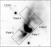 |
Fig. 2 Fields observed using Gemini-NIFS superimposed over the Ks image of YSO-G29 obtained with Gemini-NIRI. |
Observed fields using NIFS at Gemini North.
NIFS-Gemini observational parameters.
2.2 Radio observations using JVLA
We observed YSO-G29 with the JVLA at X frequency band (10 GHz; λ ~ 3 cm) in the A-array configuration (project ID: 22A–063, PI: M. Ortega), which provides the best angular resolution of the interferometer (sub arcsecond resolutions) in an FoV of about 4 arcmin. We used the full 8-12 GHz band-width with 32 spectral windows and full polarisation. As primary and secondary calibrators, 3C 286 and J1832–105 were used, respectively. The secondary calibrator is catalogued as C in the VLA calibrator source list4, which corresponds to a positional accuracy between 0.01 and 0.15 arcsecs. The total on-source integration time was 30 min. We obtained calibrated visibilities from the CASA pipeline version 5.6.2-2.el7. Additional flagging of radio frequency interference was manually performed before imaging. The image was obtained using the tclean task and Briggs weighting. We set ROBUST = 0.25 to reduce sidelobe effects from the nearby complex of bright HII regions located at ~4′ to the northwest of YSO-G29. The final image has a synthesised beam of 0.″42 × 0.″17 (FWHM), a position angle (PA) of −51.6°, and a mean noise (rms) of σrms = 6 µJy beam−1 (S/N ≥ 30). The main observational parameters are summarised in Table 3.
Additionally, we generated an image of the secondary calibrator J1832–105 (the phase calibrator) to assess the astrometric error in the final image. This source exhibits a clear point-like morphology, and its measured position was consistent with the coordinates given by the VLA calibrator source list, showing an offset of less than 0.″1.
JVLA observational parameters.
Used ALMA data.
2.3 ALMA data
The continuum emission image and data cubes from Project 2021.1.00311.S (PI: Liu, Sheng-Yuan) at Band 6 were retrieved from the ALMA Science Archive5. The single pointing observations for the target were carried out using the 34.5/226.8 telescope configuration in the 12 m array. Table 4 shows the main ALMA data parameters. The data are of QA2 quality level, which assures a reliable calibration for ‘science ready’ data. The astrometric accuracy of the data is about 3 milliarcsec (mas).
The continuum map was obtained averaging the continuum emission of each of the four spectral windows and was corrected for the primary beam. The continuum map has an rms noise level of about 0.2 mJy beam−1. The beam size of the observations (0.3 arcsec) provides a spatial resolution of about 0.009 pc (~ 1800 au) at the distance of 6.2 kpc.
3 Results
In this section we present the results from our analysis of YSO-G29. They are presented in the following subsections, according to what was obtained from the different wavelengths.
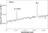 |
Fig. 3 Average spectrum obtained towards Field 1 presented as an example to show the detected near-IR lines. |
3.1 The near-IR integral field spectroscopy
In this subsection, we report the emission lines detected from the NIFS observations towards each field (Fig. 2). Continuum maps are not shown here, as they do not present any significant difference from the broad-band Ks image obtained with NIRI in our previous work (Areal et al. 2020). After inspecting the fields along the whole observed spectral range (2.009–2.435 µm), we only found Brγ and H2 S(1) 1−0 lines (rest wavelengths: 2.1661 and 2.1218 µm, respectively). Figure 3 displays, as an example, an averaged spectrum from Field 1. Both lines were detected in Fields 1 and 3, only Brγ line appears in Field 2, and no line is observed in Field 4. Figures 4, 5, and 6 exhibit maps of the observed integrated lines in each field. Figure 7 presents the H2/Brγ ratio in Field 1 at the regions in which both emissions are observed.
3.2 Discovering a compact radio continuum source
In our new radio continuum observations at 10 GHz, we detected a source located at RA=18:45:59.521, Dec= −02:45:06.618. Figure 8 displays in red contours the radio continuum emission at levels of 20 and 50 µJy beam−1. The radio emission appears as a compact source located ~0.″7 from the peak position of the central core detected at 1.3 mm (displayed in blue contours). The astrometry accuracy of JVLA and ALMA observations (see Sect. 2) confirms that this is indeed a physical separation. The flux density integrated within the 50 µJy beam−1 contour level is 0.13 ± 0.01 mJy. The complete radio image is shown in Appendix A.
3.3 The dust emission and the molecular environment
As mentioned above, Fig. 8 shows, in blue contours, the ALMA continuum emission at 1.3 mm and depicts the dust cores in the region. It is worth noting that these ALMA data provide a better resolution of such cores compared to our previous works (Areal et al. 2020; Martinez et al. 2024). The main core is the only one with a rich abundance of complex molecules. In the others, some molecules are observed, but this is mostly due to extended emission that it is centred on the main core. This indicates that these cores are colder and very probably lack protostars within them. A chemical and physical characterisation of the main dust core is included in Appendix D.
We inspected the four spectral windows (spw) from the ALMA data cubes. Apart from the many lines of complex organic molecules peaking mainly at the main core (see Appendix D), we found intense emission of 12CO, 13CO, and C18 O J=2−1 line (see Fig. 9). The systemic velocity of 101 km s−1 for the molecular core was confirmed from the C18O line. Since carbon monoxide and its isotopes effectively trace outflow activity and core envelopes, our main molecular analysis is focused on them.
To appreciate the morphology of the molecular gas in the region, as observed in carbon monoxide, we present in Fig. 10 maps of the integrated emission (moment 0) of the three CO isotopes (in green) superimposed to the Ks NIRI-Gemini emission (in red). Additionally, contours of the continuum emissions at 1.3 mm and 10 GHz are included (white and blue, respectively). The 12CO emission appears quite extended, likely depicting molecular outflows towards the south, and an intriguing shell-like feature towards the northwest. The emission of 13CO concentrates primarily at the main 1.3 mm core with some extended structures close to the peak of the near-IR emission. The C18O emission is centralised at the main core with some emission nearby.
Given the remarkable 12CO morphology observed north-westwards of the main near-IR structure – a complete shell-like feature of 2 in diameter – we present in Figs. B.1 and B.2 channel maps of the 12CO emission every 1.2 km s−1 (the spectral resolution of the observations). These channel maps show that the molecular shell-like structure extends from 87.6 to 96.0 km s−1, forming a complete and closed shell perfectly surrounded by the near-IR emission. Indeed, we can wonder whether the near-IR morphology is due to such a molecular structure, or vice versa. The velocity range from 97.2 to 102.0 km s−1, corresponding to the central and self-absorbed component of the 12CO line towards the densest region, was excluded from the analysis. Finally, from 103.2 to 108.0 km s−1, another conspicuous molecular structure extends towards the southeast. It seems to be a lobe, likely of a molecular outflow. In the first channels (103.2 and 104.4 km s−1), it appears open and composed of two structures, while from channel 105.6–108.0 km s−1, it appears collimated and quite aligned with the radio continuum source observed at 10 GHz (blue contours in the channel maps) and it coincides with the southeastern near-IR feature.
To better appreciate the red- and blue-shifted molecular gas associated with YSO-G29 we, present in Fig. 11 the 12CO emission integrated between 87.6 and 96.0 km s−1 (blue) and between 102 and 108 km s−1 (red). These integrated emissions are presented superimposed over the near-IR emission displayed in green.
Additionally, we further analysed the 13CO emission in the area where the previously described12 CO shell-like structure is observed. Figure 12 displays the 13CO integrated emission between 89.3 and 94.6 km s−1 missed in the image that presents the whole integration (Fig. 10, medium panel). This demonstrates that the observed 12CO shell is mostly filled with 13CO emission. Finally, a 12CO spectrum towards the centre of this region was extracted (black cross in Fig. 12). It is presented in Fig. 13. These results cast doubt on the nature of the observed molecular shell in 12CO, implying it might result from self-absorption or flux loss in the line signal. We address this in Sect. 4.
After confirming that the southeastern 12CO structure does not exhibit line absorption issues, we estimated the mass of the southern molecular outflow shown in Fig. 10 (upper panel), in the channel maps in Fig. B.2 (channels 102 to 108 km s−1), and in Fig. 11 (displayed in red). We obtained the 12CO column density from the 12CO J=2−1 transition following the works of Turner (1991) and Miao et al. (1995). From these studies the following equation was derived:
 (1)
(1)
where θa and θb (in arcsec) are the major and minor axes of the clean beam, respectively; W (in Jy beam−1 km s−1) is the integrated intensity; gk is the K-ladder degeneracy; gl is the degeneracy due to the nuclear spin; ν0 (in gigahertz) is the rest frequency of the transition; Sul is the line strength of the transition; µ0 (in Debye) is the permanent dipole moment of the molecule; Eu/k is energy of the upper level; and Tex is the excitation temperature.
From the moment zero map of the outflow structure, we estimated an integrated intensity of about 0.5 Jy beam−1 km s−1. Thus, assuming Tex = 20 K and using the transition and molecular parameters obtained from the Splatalogue Database for Astronomical Spectroscopy (SDAS)6, we derived an average 12CO column density of about 6.7 × 1016 cm−2.
We estimated the total mass of the molecular outflow using the following equation:
![Mathematical equation: ${{\rm{M}}_{{\rm{out}}}} = {\rm{N}}\left( {^{12}{\rm{CO}}} \right)\left[ {{{\rm{H}}_2}/{\rm{CO}}} \right]\,\,{\mu _{{{\rm{H}}_2}}}\,{{\rm{m}}_{\rm{H}}}\,{{\rm{A}}_{{\rm{pixel}}}}\,{{\rm{N}}_{{\rm{pixel}}}},$](/articles/aa/full_html/2025/10/aa55716-25/aa55716-25-eq2.png) (2)
(2)
where N(12CO) is the average column density of the lobe, [CO/H2] = 10−4 is the abundance ratio between the molecules,  is the mean molecular weight, mH = 1.67 × 10⁻²⁴ g is the mass of the hydrogen atom, Apixel is the pixel area, and Npixel is the number of pixels that fills the lobe. Using the distance of 6.2 kpc to YSO-G29, we obtained a mass for the outflow of about 0.2 M⊙.
We then estimated the outflow rate (Ṁ = Mout/tdyn), momentum  , and outflow momentum rate (Ṗ = P/tdyn). We obtained the dynamical time (tdyn) from L/υmax, where L is the length of the outflow (about 0.06 pc), and
  and υmax are the median and maximum velocity with respect to the systemic velocity. The following values were obtained: tdyn ~ 8.3 × 10³ yr, Ṁ = 2.4 × 10⁵ M⊙ yr−1, P ~ 0.8 M⊙ km s−1, and Ṗ ~ 1 × 10⁻⁴ M⊙ km s−1 yr−1. Caution is advised when interpreting these values due to potential projection effects. The small velocity range indicates that such an outflow is observed mainly along the plane of the sky. In that case, the derived values for P and Ṗ should be considered lower limits.
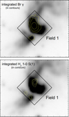 |
Fig. 4 Integrated Brγ and H2 1−0 S(1) emissions (continuum subtracted) towards Field 1 (yellow contours) superimposed over the Ks image obtained with NIRI. The contour levels are 1.3, 2.1, and 4.0 ×10⁻¹⁹ erg s−1cm−2 for the Brγ line, whereas they are 2.6, 3.0, and 3.8 ×10⁻¹⁹ erg s−1cm−2 for the H2 1−0 S(1) line. In both cases, the first contour is above 4σ. Box area is 3″ × 3″. |
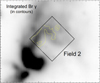 |
Fig. 5 Integrated Brγ emission (continuum subtracted) towards Field 2 (yellow contours) superimposed over the Ks image obtained with NIRI. The contour levels are 0.7 and 1.2 ×10⁻¹⁹ erg s−1cm−2. The first contour is above 4σ. Box area is 3″ × 3″. |
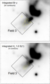 |
Fig. 6 Integrated Brγ and H2 1−0 S(1) emissions (continuum subtracted) towards Field 3 (yellow contours) superimposed over the Ks image obtained with NIRI. The contour levels are 2.2 and 5.0 for the Brγ line, whereas they are 0.6, 1.0, and 2.0 ×10⁻¹⁹ erg s−1 cm−2 for the H2 1−0 S(1) line. In both cases, the first contour is above 4σ. Box area is 3″ × 3″. |
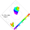 |
Fig. 7 Ratio of H2/Brγ in Field 1. Black (solid) and blue (dashed) contours are the lowest contours of the H2 and Brγ integrated emissions, respectively, presented in Fig. 4. These contours are displayed for reference. |
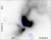 |
Fig. 8 Ks image presented in our previous work obtained with NIRI at Gemini North (Areal et al. 2020). Blue contours represent the continuum emission at 1.3 mm obtained with ALMA at levels 1.8, 2.4, 4.0, and 8.0 mJy beam−1 (rms = 0.2 mJy beam−1). Radio continuum emission at 10 GHz acquired with JVLA is presented in red contours with levels of 20 and 50 µJy beam−1 (rms = 6 µJy beam−1). The beams of the ALMA and JVLA observations (blue and red) are presented at the top-right corner. |
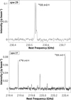 |
Fig. 9 Portions of spectra from the spectral windows spw29 (up) and spw27 (bottom) obtained from a beam centred at the peak of the main dust core shown in Fig. 8. The lines of the 12CO (upper spectrum) and C18O and 13CO (bottom spectrum) are indicated. |
 |
Fig. 10 Two-colour maps of the YSO-G29 region. In green is displayed the 12CO, 13CO, and C18O J=2−1 emissions integrated along the whole frequency/velocity range in which each line extends as presented in Fig. 9. The Ks emission obtained with NIRI-Gemini is shown in red. White contours represent the continuum emission at 1.3 mm (same levels as Fig. 8), and blue contours are the continuum emission at 10 GHz (same levels as Fig. 8). The units of the colour bars at the right of each image are Jy beam−1 km s−1 and correspond to the green colour of the maps. The rms noise level of the molecular integrated emission is about 0.15 Jy beam−1 km s−1 for the three maps. |
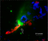 |
Fig. 11 12CO J=2−1 integrated in the velocity ranges 87.6–96.0 and 102–108 km s−1 displayed in blue and red, respectively. The NIRI near-IR emission is displayed in green. The contour levels are 0.37, 0.50, and 0.75 Jy beam−1 km s−1 for the blue emission and 0.50, 0.75, and 1.00 Jy beam−1 km s−1 for the red emission. The white and black contours are the continuum emission at 1.3 mm and 10 GHz as presented in previous figures. |
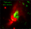 |
Fig. 12 13CO J=2−1 integrated between 89.3 and 94.6 km s−1 with contours with levels of 0.095, 0.150, and 0.200 Jy beam−1 km s−1. The rms noise level of the integrated map is 0.030 Jy beam−1 km s−1. The black cross represents the position from which the 12CO spectrum shown in Fig. 13 was extracted. |
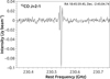 |
Fig. 13 12CO J=2−1 spectrum obtained towards the region indicated with the black cross in Fig. 12 (coordinates are indicated in the top right-corner). |
4 Discussion
With a new set of high-quality data at higher angular resolutions than previous studies, we propose a compelling new scenario for the intriguing morphology of YSO-G29. This analysis provides valuable observational insights into star formation processes.
4.1 Near-IR emission: Lines from Gemini-NIFS
The new Gemini-NIFS near-IR data reveal H2 1−0 S(1) and Bγ emission towards the main near-IR structure and the southern smaller feature (Figs. 4 and 6, respectively) previously observed with Gemini-NIRI. On the other hand, only the Brγ feature is detected to the north (Fig. 5). No other lines at near-IR were observed.
The hydrogen Brγ emission line is commonly observed towards massive YSOs (e.g. Cooper et al. 2013). Here, the extended emission observed in Fields 1, 2, and 3, which has a morphological correspondence with the continuum emission, strongly suggests that this line arises from stellar strong winds (Fedriani et al. 2019) probably extending along cavities cleared out by jets.
Conversely, it is well known that the excitation of H2 1−0 S(1) can be due to collisions or UV fluorescence. Ratios among different H2 near-IR lines are typically used to distinguish between excitation mechanisms (e.g. Paron et al. 2022). However, the 1−0 S(1) is the only H2 line detected in our observations. By comparing the regions in which H2 is detected with their corresponding Brγ emission in Field 1, we find that the H2 1−0 S(1)/Brγ ratio presents a gradient going from values less than one to somewhat larger than the unity at the main region of near-IR emission (see Fig. 7). This suggests a combination of excitation mechanisms for the H2 emission in the region: UV excitation (ratios < 1) and shocked gas (ratios > 1) (see Hatch et al. 2005; Chen et al. 2015; Reiter et al. 2024). For its part, the southern near-IR structure in Field1 presents H2/Brγ ratios larger than one, suggesting that this H2 feature is due to shocked gas.
We conclude that the detected near-IR lines are compatible with excitation and ionisation from UV radiation propagating in a highly perturbed ambient by the activity of YSO-G29, with some contribution of shocked gas. It should be emphasised that no line at near-IR was detected towards the dark lane (see Fig. 1) purported to be a disc or a toroid of material observed edge-on in Areal et al. (2020). As spectral lines can be detected towards discs and/or toroids (e.g. Murakawa et al. 2013), we ruled out such a nature for the dark lane, proposing it to be just a region lacking near-IR emission.
4.2 Molecular outflows
Using ALMA data in band 6 with an angular resolution of 0.″3, we discovered molecular outflows associated with YSO-G29 (systemic velocity about 101 km s−1) at small spatial scales (resolving structures of about 1800 au). This discovery also challenges the conclusions drawn in Areal et al. (2020) regarding the red- and blue-shifted jets and outflows.
We discovered a conspicuous 12CO outflow extending south-eastwards (see Figs. 10, B.2, and 11). Considering the velocity range over which this outflow extends, although not particularly broad, we infer that it is a red-shifted outflow. Hence, the features observed northwestwards can be attributed to blue-shifted gas (see Figs. B.1 and 11), conforming a more open and fragmented structure. Changing the scenario regarding the directions of jets and outflows proposed in Areal et al. (2020), we conclude that, at present, the observed extensions of the near-IR features make sense: the northern-southern asymmetry in the extension of the structures observed at the Ks broad-band should partially be due to possible extinction effects that are more pronounced in the southern red-shifted feature.
The southern CO outflow appears quite collimated and somewhat clumpy along the line of sight. For instance, in velocity channels at 102.0, 103.2, and 104.4 km s−1 (see Fig. B.2), the out-flow seems to be composed of two structures: one more aligned with the main millimetre core and the other along the same direction of the radio continuum source. In velocity channels at 105.6 and 106.8 km s−1, the outflow presents a well-collimated structure aligned mostly towards the position of the radio continuum source. Notably, in these velocity channels, the CO emission seems to originate at the position of the main millimetre core, extending southwards before bending to the southeast, where it forms the collimated outflow previously mentioned.
The obtained mass of such a southern molecular outflow, about 0.2 M⊙, is in agreement with the mass of many CO out-flows associated with cores embedded in massive 70 µm dark clumps (Li et al. 2020). It is worth mentioning that the mentioned authors carried out a statistical study of molecular outflows using ALMA observations based on the 12CO J=2−1 line, and they found a median outflow velocity of about 21 km s−1 with respect to the systemic velocity. Therefore, the low velocity of the YSO-G29 southern outflow, about 4 km s−1, indicates that this molecular feature should extend mostly along the plane of the sky, confirming that P and Ṗ should be lower limits. More-over, one must also be careful with the parameters obtained, as the analysed outflow may be the product of outflows from more than one source.
Regarding the northern-northwestern molecular ambient, there does not appear to be any collimated feature as in the southern region. On the contrary, we found fragmented molecular gas, with the most remarkable features being a quite extended CO shell-like structure with an excellent morphological correspondence with the near-IR emission from Gemini-NIRI (see Fig. 10 upper panel, channels from 87.6 to 94.8 km s−1 in Figs. B.1 and 11). However, the presence of a 13CO structure contained by such a 12CO shell-like structure (Fig. 12) also perfectly matching with the near-IR emission casts doubt on the shell nature of the molecular gas. Indeed, the 12CO spectra towards the centre of this structure are highly absorbed (Fig. 13). This can be due to the high optical depth effects that 12CO lines usually suffer in dense gaseous structures. Additionally, the deep 12CO absorption spectral feature could indicate missing flux coming from more extended spatial scales that are filtered out by the interferometer. Certainly, this phenomenon can produce not only missing flux but also deep absorption features (e.g. Choi et al. 2004; Rodón et al. 2012; Paron et al. 2021). We conclude that the observed structure is not a molecular shell enclosed by near-IR emission but a non-collimated molecular outflow component likely produced by one or multiple ejections from YSO-G29 that have impacted the feature observed in the near-IR.
The near-IR emission related to YSOs at these small spatial scales usually has a cone-shaped nebulae morphology. This is due to cavities cleared out in the circumstellar material by the action of jets and winds, which are bright mainly at near-IR (Reipurth et al. 2000; Bik et al. 2005; Paron et al. 2013, 2016; Sanna et al. 2019). It could be the case of YSO-G29, and taking into account the perfect morphological correspondence between the molecular emission and the intriguing morphology of the northern near-IR feature, we suggest that an ejection of molecular gas could have disrupted a previously carved cone-shaped cavity. We discuss this further in Sect. 4.4.
4.3 Radio continuum source
Weak and compact radio sources in star-forming regions may be associated with HII regions in their earlier stages of evolution (namely, HC/UC HII regions), where thermal radio emission forms as a consequence of photoionisation by a recently born star. Alternatively, radio emission may be associated with jets of YSOs, where thermal free–free emission arises as a consequence of shock ionisation in the wind or jet of the protostars. In some cases, these so-called ionised jets trace the base of the jet (i.e. they trace the position of the powering protostar), while in other cases they form in knots along the jet away from the protostar. The most powerful knots, where strong shocks arise, can also be sources of non-thermal radio emission of synchrotron origin, which are sometimes referred to as non-thermal lobes (see Anglada et al. 2018 for a review of radio jets in YSOs).
In an attempt to classify our discovered compact radio source, we compared the radio luminosity (Sν D2) and the bolo-metric luminosity (Lbol). Anglada et al. (1992) found that the Sν D2 of ionised jets is positively correlated with Lbol, and sub-sequent surveys in the radio band have confirmed that this correlation is valid for both low- and high-mass protostars (see Purser et al. 2016; Rosero et al. 2019; Purser et al. 2021). Following Purser et al. (2021), we extrapolated our radio flux at 10 GHz to 5.8 GHz while assuming some spectral behaviour and estimated the radio luminosity for a distance of D = 6.2 kpc. For an ionised jet or knot, we took a canonical spectral index of α = 0.6, while for a HC/UC HII region, we used α = −0.1, which is the theoretical value of a photoionised nebula in the optically thin regime. We obtained S58D2 = 3.5 and 5.2 mJy kpc2 for α = 0.6 and −0.1, respectively. Regarding the bolometric luminosity of the region, we estimated Lbol ~ 3.7 × 10⁴ L⊙ following the method presented in Rosero et al. (2019) (see Appendix C).
In Fig. 14, we show the S5.8 D2 versus Lbol diagram of Purser et al. (2021) (see their Figure 4), where we have included our compact radio source (yellow dot crossed by dashed lines)7. The figure shows that the compact radio source is located in the region of the diagram populated by ionised jets and non-thermal lobes from high-mass protostars. However, taking into account the large dispersion of the diagram and the possibility that multiple sources in the region contribute to Lbol, we could not rules out the fact that the compact radio source may be a HC/UC HII region. Indeed, if ~3.7 × 10 L⊙ is an upper limit to the bolometric luminosity of the radio source, its actual position in the diagram may be displaced in the direction of the Lyman continuum of a zero age main sequence star. By considering the possibility of an HII region, we could estimate the Lyman continuum photon flux of the putative star responsible for the ionisation. From Kurtz et al. (1994), using the radio flux at 10 GHz (Sν = 86 µJy), Te = 104 K and the parameter a = 1, we derived NLy, = 3.2 × 1044 ph s−1. Following Avedisova (1979), this amount of Lyman photons should be produced by a B1 type star.
In summary, our analysis of the available information about the radio compact source points to single-source and multiple-source scenarios for the YSO-G29 region. In the former, the compact radio source may be a thermal knot or a non-thermal lobe located along the jet of a putative protostar likely situated at the centre of the 1.3 mm core (the unique core with high temperatures in the region). In the multiple-source scenario, the ALMA main core may host a massive protostar, while the radio source may indicate the position of a second massive young star: either a massive protostar powering an ionised thermal jet (which traces the base of the jet, i.e. the position of the powering protostar) or an HC/UC HII region excited by a B1 type star. Conducting a radio spectral index study would provide valuable insights for discerning the nature of the radio source. Based on these possibilities, the following section explores the most plausible interpretation for this region, focusing on the complex morphology observed mainly at near-IR and the molecular emission distribution.
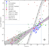 |
Fig. 14 Reproduction of Fig. 4 from Purser et al. (2021): radio luminosity (S νd2) vs. bolometric luminosity (Lbol). Our source is indicated with a yellow circle crossed by dashed lines. |
4.4 Proposed scenario for YSO-G29
As shown above, the discovered radio continuum emission could be an UCHII region, an ionised jet from a massive object, or even a non-thermal lobe. This last possibility would suggest that it should be a jet coming from an undetected object embedded in the main molecular core. Notably, a similar case has been reported in Beltrán et al. (2016). However, taking into account the complexity of the morphology of the different emissions, hereafter we favour a scenario of multiple YSOs in the region.
Given that the radio continuum source is not associated with a peak of a molecular core (traced by dust emission), we suggest that it is more likely to be an UCHII region than an ionised jet from a massive object. Such an UCHII region would probably have evacuated the surrounding dust. Then, taking into account that the main 1.3 mm core is the only one in the region with a rich presence of complex organic molecules peaking at its maximum (it has indeed high temperatures; see Appendix D), we propose that this core and the discovered radio continuum source are the sole objects related to active star formation in the region. Hence, the positional offset between them merits further discussion.
Assuming the main core must contain an internal heat source, we propose the existence of a protostar or a non-detected massive star embedded within it. Considering the latter case, from the rms noise level of the radio continuum image, we can roughly estimate an upper limit of Lyman photons emanating from such a star and then estimate an upper limit for its spectral type. Following the same procedure as described above for the compact radio source, we obtained an amount of ionising photons of NLy = 2.2 × 1043 ph s−1 from considering a flux density equal to the rms noise level of the radio image. Then, based on Avedisova (1979), we concluded that the spectral type of the putative star could be B3 or later, i.e. a star with a lower or a much lower mass than the star responsible of the detected radio compact source. Of course, the object embedded in this core could be a young protostar that has not begun to ionise the surrounding gas yet.
In addition, it is worth noting that the Brγ emission detected at near-IR with Gemini-NIFS (see Sect. 4.1) shows the presence of ionised gas in the region, reinforcing the hypothesis of ionising sources, which indeed could be young HII regions. Even though the Brγ peak is not coincident with the position of the radio continuum source proposed to be an UCHII region, it may indicate ionised gas escaping from it, with some contribution from the source embedded in the dust main core. In conclusion, a crucial finding of this study is the identification of a likely YSO binary system.
It is known that binary and multiple systems are a common outcome of the star formation process (Ricciardi et al. 2025, and references therein). YSO-G29 could be a binary system composed of a star later than B3 or a non-ionising protostar and a B1 type star generating an UCHII region. If this is the case, the observed system would present a projected separation of 0.02 pc (about 4000 au) between the two stellar components. Following Ricciardi et al. (2025), this could be a probable separation for a wide binary system, likely generated by turbulent fragmentation of a molecular cloud. In such a case, assuming both stars began forming at the same time and considering that massive stars form more rapidly, the mass difference between the two objects is consistent with the less evolved stage of the embedded one. Additionally, it is important to note that if the embedded source in the core is a protostar, it is likely that it will not become a massive star (see the estimated mass for the core in Appendix D).
The scenario of a wide binary system would explain the morphology of the different features detected in infrared and molecular lines. For instance, the observed structures of the molecular outflows (see Figs. B.1 and B.2, and Sect. 4.2) would be due to ejections originating from both objects. What is indeed outstanding is the perfect morphological matching between the molecular gas and the near-IR emission towards the northwest (see Figs. B.1, 11 and 12). Given that it is normal to detect cone-like near-IR features towards YSOs tracing cavities cleared out in the circumstellar material by the action of jets and winds (Reipurth et al. 2000; Bik et al. 2005; Paron et al. 2013, 2016; Sanna et al. 2019), we are probably observing this type of cavity but one that was disrupted at the western part.
Thus, it is probable that one of the sources generated the mentioned cavity and that molecular outflows from the other source subsequently disrupted it. This proposed scenario could finally elucidate the infrared structure associated with YSO-G29, which has remained virtually unexplained since our initial study focusing on this region published in 2020 (Areal et al. 2020).
This type of interaction might be relatively common in star-forming regions with multiple components (see Bally 2016, and references therein). For instance, Zapata et al. (2018) have described the collision between two outflows in a protostar binary system. Our case resembles this scenario, as a YSO circumstellar cavity is being disrupted by an outflow in this reported collision. These kinds of interactions and disruptions are important phenomena to consider when studying massive star-forming regions with high angular resolutions.
5 Conclusion
Using a new set of high-quality multi-wavelength data, we set out to shed light on YSO G29.862-0.0044 (YSO-G29). The most intriguing aspect was the morphology that the YSO presents in near-IR, which was observed more than five years ago with Gemini-NIRI. We conclude that the results presented in this work may resolve this question, and they can provide valuable observational evidence for our understanding of star-forming regions that exhibit high confusion.
From the discovery of a compact radio source and the analysis of a hot molecular core with a probable stellar object embedded within it, we found evidence of a YSO binary system that has one component that may have generated a cavity in the surrounding interstellar medium. Our most significant result is the observational evidence that such a cavity was partially disrupted by a molecular outflow likely generated by the other component of the YSO binary system. This would be a similar case to others reported in the literature regarding collisions of outflows and cavity disruptions.
These results obtained from highly detailed observations of a distant star-forming site (about 6.2 kpc) not only help complete the picture of what is happening in this particular region, but also reveal an interesting disruption phenomenon. This is something of importance to be considered when investigating high-mass star-forming regions that exhibit high confusion.
Acknowledgements
We thank the anonymous referee for her/his insightful comments and suggestions that helped us to improve this work. N.C.M. is a doctoral fellow of CONICET, Argentina. This work was partially supported by the Argentine grants PIP 2021 11220200100012 and PICT 2021-GRF-TII-00061 awarded by CONICET and ANPCYT. This work is based on the following ALMA data: ADS/JAO.ALMA # 2021.1.00311.S. ALMA is a partnership of ESO (representing its member states), NSF (USA) and NINS (Japan), together with NRC (Canada), MOST and ASIAA (Taiwan), and KASI (Republic of Korea), in cooperation with the Republic of Chile. The Joint ALMA Observatory is operated by ESO, AUI/NRAO and NAOJ.
Appendix A Radio image
In Fig. A.1, we show the JVLA radio continuum image at 10 GHz, covering the FoV of ALMA observation. Figure A.2 shows a zoomed-in image of the compact radio source.
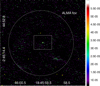 |
Fig. A.1 Radio continuum emission at 10 GHz. The white circle is ALMA’s FoV and the white rectangle is the zoomed-in region shown in Fig. A.2. Colour scale is expressed in Jy beam−1 and goes from 6 to 60 µJy beam−1, corresponding to 1 and 10 times the image noise (σrms = 6 µJy beam−1), respectively. Countor levels are: −3σrms (yellow), 2σrms (green), and 3σrms (red). |
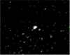 |
Fig. A.2 Zoomed-in view of the compact radio source. Contour levels are: 2σrms (green), 3σrms (red), 5σrms (cyan), and 10σrms (magenta). |
Appendix B 12CO emission in velocity channels
In this appendix we include the channel maps of the 12CO J=2−1 emission (Figs. B.1 and B.2).
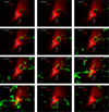 |
Fig. B.1 12CO J=2−1 channel maps towards YSO-G29 in green contours with levels of 0.075, 0.100, and 0.150 Jy beam−1. Ks emission from NIRI-Gemini is displayed in red. Contours of the continuum emissions at 1.3 mm (white) and at 10 GHz (blue) are included (same levels as the above figures). Maps continue in Fig. B.2. The rms noise level of each 12CO channel is 0.025 Jy beam−1. The systemic velocity of the source is 101 km s−1. |
Appendix C Bolometric luminosity of the region
We estimated the bolometric luminosity of the region following the same procedure of R19, who used a linear interpolation of the fluxes between the mid-IR and the millimetre bands. In Table C.1 we report the fluxes ƒλ of the catalogued sources from the Bolocam Galactic Plane Survey (BGPS, Rosolowsky et al. 2010), the APEX Telescope Large Area Survey of the Galaxy (ATLAS-GAL, Urquhart et al. 2014), and the Herschel Space Observatory infrared Galactic Plane Survey (Hi-GAL, Molinari et al. 2016). In the mid-IR band, R19 used the 24 µm flux from the MIPS-GAL survey, but in our case the catalogued source MIPSGAL MG029.8569-00.0434 overlaps with a masked out area of the MIPSGAL image, probably due to saturation. Instead, we used the flux at 22 µm of the Wide-field Infrared Survey Explorer (allWISE, Cutri et al. 2021). In Fig. C.1 we show the spectral energy distribution and the linear interpolation. The area under the interpolation gives the bolometric flux A = (3.06 ± 0.01) × 10−8 erg s−1 cm−2. To estimate the error, we obtained a lower and an upper limits of the area by interpolating ƒλ − ∆ƒλ and ƒλ + ∆ƒλ, respectively, where ∆ƒλ are the fluxes errors of Table C.1. For a distance d = 6.2 ± 0.6 kpc, the bolometric luminosity is Lbol = 4πAd2 = (3.7 ± 0.7) × 104 L⊙.
Mid-IR, submillimetre and millimetre fluxes ƒλ in the direction of YSO-G29.
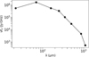 |
Fig. C.1 Spectral energy distribution in the mid-IR, submillimeter and millimeter bands in the direction of YSO-G29. The bolometric flux of the region is estimated as the area under the linear interpolation of the fluxes. |
Appendix D Chemical and physical characterisation of the main dust core
To complement the multi-wavelength characterisation of YSO-G29, we examined the chemical composition of the main dust core revealed by the ALMA observations, the only one in the region with noticeable emission of complex organic molecules. Hot molecular cores such as G29 generally have elevated temperatures, high densities, and a rich molecular content. The extreme conditions cause the ice on the dust grains to sublimate, releasing molecules into the gas phase and initiating complex chemical reactions. Molecular composition studies of these environments provide insight into both the physical conditions of the gas and the formation pathways of complex organic molecules.
In this context, we conducted a detailed spectral analysis of the ALMA Band 6 data to identify the molecular species in the hot core associated with YSO-G29. This study integrates spectral data from two independent datasets: Project 2021.1.00311.S (PI: Liu, Sheng-Yuan), mentioned in Sect. 2.3, and Project 2015.1.01312.S (PI: G. Fuller), described in Ortega et al. (2023). These observations provide complementary coverage of the 216.6–242.7 GHz frequency range, distributed across eight spectral windows. Spectra were extracted from them using a circular region centred at the continuum emission peak (see green dashed circle in Fig. D.1). We visually inspected each spectrum to identify molecular lines and labelled all distinguishable features. Molecular identification was performed using the SDAS, considering the rest frequency, line strength, upper-level energy, and molecular species. This process led to identifying a chemically rich inventory displayed in Figs. D.2 and D.3. It includes both simple and complex species such as CH3CN, HC3N, H2CO, HNCO, CN, SO, SO2, and various isotopologs, among others.
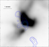 |
Fig. D.1 Ks Gemini-NIRI image with ALMA continuum at 1.3 mm contours as presented above. The green dashed circle indicates the position from which spectra presented in Figs. D.2 and D.3 were extracted. |
The rotational diagram analysis was carried out for certain detected molecules −CH3CN, CH3CCH, E-CH3OH, A-CH3OH, HC3N, and CH3OCH3− that exhibit at least two unblended transitions accompanied by well-characterised upper-level energies (Eu) and integrated intensities. Following the formalism described in Ortega et al. (2023) (see their Sect. 4.3.1.) we computed the natural logarithm of the column density per statistical weight (ln(Nu/gu)) as a function of the Eu (Fig. D.4). This calculation used the integrated line intensities, beam dimensions, and spectroscopic parameters retrieved from the SDAS, which compiles spectroscopic constants from the Cologne Database for Molecular Spectroscopy (CDMS) and Jet Propulsion Laboratory Molecular Spectroscopy (JPL) catalogs. Under the assumptions of local thermodynamic equilibrium (LTE) and optically thin emission, the inverse of the slope of the linear fit yields the rotational temperature (Trot). In this approximation Trot is considered a proxy for the kinetic temperature (Tk) of the gas.
The derived rotational temperatures span a wide range, from approximately 70 K to over 360 K, indicating that chemically distinct species trace gas layers with varying thermal conditions within the hot core. The derived Trot for CH3CN and HC3N are 361 K and 236 K, respectively. These values are consistent with those reported in previous studies of hot molecular cores. For instance, Ortega et al. (2023) found that CH3CN traces gas layers with temperatures around 340 K, indicating its association with the innermost, hottest regions of the core. Similarly, Chen et al. (2025) reported rotational temperatures for HC3N in the range of 160–335 K, with a mean value of 235 K, in excellent agreement with our result. However, it is important to note that their analysis was based on vibrationally excited transitions of the molecule, while in our case, only the ground state was considered. Although we did not detect vibrationally excited lines of this molecule, their presence in the region cannot be ruled out. Therefore, obtaining a similar temperature from ground-state transitions is plausible and consistent with the presence of compact warm gas. It should be noted that our HC3N fit is based on only two transitions. Although the derived Trot is consistent with previous high-resolution studies, additional data would be necessary to confirm this estimate with higher confidence.
The detection of vibrationally excited transitions of CH3CN (v8 = 1) and CH3OH (vt = 1) provides further evidence of hot, compact gas near the central source. These lines are typically excited in regions with temperatures above ~ 200–300 K and have been observed in well-studied hot cores such as Orion (Sutton et al. 1986) and in star-forming regions such as G9.62+0.19 (Peng et al. 2022). These detections in YSO-G29 indicate the presence of deeply embedded, high-excitation gas layers, consistent with physical conditions near a massive protostar.
Both Trot obtained for CH3OH in their A and E configurations indicate that this molecule probes gas found at moderate temperatures in the core. A more detailed analysis of the relative behaviour of the A/E symmetry states and their implications for the thermal and chemical structure of the source is discussed in Martinez et al. (in prep.). On the other hand, CH3CCH and CH3OCH3 appear to trace colder gas components within the hot core environment. Both molecules exhibit lower rotational temperatures in our analysis, suggesting that their emission originates from more extended and less heated regions of the core. CH3CCH, in particular, has been widely used as a tracer of lukewarm gas in dense molecular clouds and hot cores, often reflecting temperatures in the 30-100 K range (Santos et al. 2022; Ortega et al. 2023). Similarly, CH3OCH3 is typically associated with chemically evolved gas released into the gas phase through thermal desorption. However, it can persist in cooler layers, especially if it forms on grain surfaces and is desorbed early during the heating phase, where it is found to trace similar temperatures (Fontani et al. 2007; Li et al. 2024). The relatively low excitation temperatures derived for CH3OCH3 in YSO-G29 are therefore consistent with an origin in the outer and cooler regions of the hot core—likely within the envelope—where complex organic molecules may survive for longer periods before being further processed or destroyed. In addition, sulfur-bearing species such as SO, SO2, and H2CS were also identified, highlighting the chemical diversity of the region and suggesting active sulfur chemistry operating in this range of physical conditions.
In summary, the molecular inventory and excitation analysis of YSO-G29 reveal a chemically rich and thermally stratified hot core. The range of rotational temperatures derived from species probing different excitation regimes—ranging from compact, high-temperature gas to cooler, more extended components—points to the presence of a radial thermal gradient, as expected in internally heated protostellar environments. The detection of vibrationally excited transitions and complex organics further supports the advanced chemical evolution of the core.
As a final step in the physical characterisation of the chemically rich core, we estimated its mass using the approach described by Kauffmann et al. (2008) (eq. B.1):
![Mathematical equation: $\eqalign{ & {{\rm{M}}_{{\rm{gas}}}} = 0.12\,{{\rm{M}}_ \odot }\left[ {\exp \left( {{{1.439} \over {\left( {\lambda /{\rm{mm}}} \right)\left( {{{\rm{T}}_{{\rm{dust}}}}/10\,{\rm{K}}} \right)}}} \right) - 1} \right] \cr & \,\,\,\,\,\,\,\,\,\,\, \times {\left( {{{{\kappa _v}} \over {0.01\,{\rm{c}}{{\rm{m}}^2}\,{{\rm{g}}^{ - 1}}}}} \right)^{ - 1}}\left( {{{{{\rm{S}}_v}} \over {{\rm{Jy}}}}} \right){\left( {{{\rm{d}} \over {{\rm{100 pc}}}}} \right)^2}{\left( {{\lambda \over {{\rm{mm}}}}} \right)^3} \cr} $](/articles/aa/full_html/2025/10/aa55716-25/aa55716-25-eq7.png) (D.1)
(D.1)
We used the integrated flux at 1.3 mm, Sν = 0.03 Jy, and assumed a dust temperature, Tdust = 361 K, derived from the CH3CN emission and considering the thermal coupling of gas and dust. The dust opacity per gram of matter at 1.3 mm, κν, was adopted as 0.013 cm2 g−1 (Lin et al. 2021). The resulting mass is approximately 1 M⊙, for a distance of 6.2 kpc.
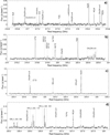 |
Fig. D.2 Spectra of the eight spectral windows analysed in this study. Panels a), b), e), and f) present data obtained from the observations reported by Liu et al. (Project 2021.1.00311.S), whereas panels c), d), g), and h) correspond to the dataset acquired by Fuller et al. (Project 2015.1.01312.S). Each spectrum was extracted from a beam-size region centred at the peak of the continuum emission. Molecular transitions were identified using the SDAS database. |
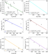 |
Fig. D.4 Rotational diagrams of selected molecules towards YSO-G29: (a) CH3CN, (b) HC3N, (c) E − CH3OH, (d) A − CH3OH, (e) CH3OCH3, and (f) CH3CCH. Panels c), d), and f) are reproduced from Martinez et al. (2025, in prep.). The coloured lines represent the best linear fit of each dataset. For HC3N, the uncertainty of the rotational temperature was not estimated due to insufficient degrees of freedom. |
References
- Anglada, G., Rodriguez, L. F., Canto, J., Estalella, R., & Torrelles, J. M. 1992, ApJ, 395, 494 [NASA ADS] [CrossRef] [Google Scholar]
- Anglada, G., Rodriguez, L. F., & Carrasco-González, C. 2018, A&A Rev., 26, 3 [Google Scholar]
- Areal, M. B., Paron, S., Fariña, C., et al. 2020, A&A, 641, A104 [NASA ADS] [CrossRef] [EDP Sciences] [Google Scholar]
- Areal, M. B., Paron, S., Fariña, C., et al. 2021, A&A, 651, C1 [NASA ADS] [CrossRef] [EDP Sciences] [Google Scholar]
- Avedisova, V. S. 1979, Soviet Ast., 23, 544 [NASA ADS] [Google Scholar]
- Bally, J. 2016, ARA&A, 54, 491 [Google Scholar]
- Bayo, A., Rodrigo, C., Barrado Y Navascués, D., et al. 2008, A&A, 492, 277 [NASA ADS] [CrossRef] [EDP Sciences] [Google Scholar]
- Beltrán, M. T., Cesaroni, R., Moscadelli, L., et al. 2016, A&A, 593, A49 [NASA ADS] [CrossRef] [EDP Sciences] [Google Scholar]
- Beuther, H., Kuiper, R., & Tafalla, M. 2025, arXiv e-prints [arXiv:2501.16866] [Google Scholar]
- Bik, A., Kaper, L., Hanson, M. M., & Smits, M. 2005, A&A, 440, 121 [NASA ADS] [CrossRef] [EDP Sciences] [Google Scholar]
- Bonfand, M., Belloche, A., Garrod, R. T., et al. 2019, A&A, 628, A27 [NASA ADS] [CrossRef] [EDP Sciences] [Google Scholar]
- Caratti o Garatti, A., Stecklum, B., Linz, H., Garcia Lopez, R., & Sanna, A. 2015, A&A, 573, A82 [NASA ADS] [CrossRef] [EDP Sciences] [Google Scholar]
- Carlhoff, P., Nguyen Luong, Q., Schilke, P., et al. 2013, A&A, 560, A24 [NASA ADS] [CrossRef] [EDP Sciences] [Google Scholar]
- Chen, Z., Nürnberger, D. E. A., Chini, R., Jiang, Z., & Fang, M. 2015, A&A, 578, A82 [NASA ADS] [CrossRef] [EDP Sciences] [Google Scholar]
- Chen, L., Qin, S.-L., Liu, T., et al. 2025, A&A, 694, A166 [NASA ADS] [CrossRef] [EDP Sciences] [Google Scholar]
- Choi, M., Kamazaki, T., Tatematsu, K., & Panis, J.-F. 2004, ApJ, 617, 1157 [Google Scholar]
- Cooper, H. D. B., Lumsden, S. L., Oudmaijer, R. D., et al. 2013, MNRAS, 430, 1125 [NASA ADS] [CrossRef] [Google Scholar]
- Cutri, R. M., Wright, E. L., Conrow, T., et al. 2021, VizieR On-line Data Catalog: II/328 [Google Scholar]
- Fedriani, R., Caratti o Garatti, A., Coffey, D., et al. 2018, A&A, 616, A126 [NASA ADS] [CrossRef] [EDP Sciences] [Google Scholar]
- Fedriani, R., Caratti o Garatti, A., Purser, S. J. D., et al. 2019, Nat. Comm., 10, 3630 [Google Scholar]
- Ferrero, L. V., Günthardt, G., Garcia, L., et al. 2022, A&A, 657, A110 [NASA ADS] [CrossRef] [EDP Sciences] [Google Scholar]
- Fontani, F., Pascucci, I., Caselli, P., et al. 2007, A&A, 470, 639 [NASA ADS] [CrossRef] [EDP Sciences] [Google Scholar]
- Gredel, R. 2006, A&A, 457, 157 [NASA ADS] [CrossRef] [EDP Sciences] [Google Scholar]
- Hatch, N. A., Crawford, C. S., Fabian, A. C., & Johnstone, R. M. 2005, MNRAS, 358, 765 [NASA ADS] [CrossRef] [Google Scholar]
- Herbst, E., & van Dishoeck, E. F. 2009, ARA&A, 47, 427 [NASA ADS] [CrossRef] [Google Scholar]
- Jørgensen, J. K., Belloche, A., & Garrod, R. T. 2020, ARA&A, 58, 727 [Google Scholar]
- Kauffmann, J., Bertoldi, F., Bourke, T. L., Evans, N. J., I., & Lee, C. W. 2008, A&A, 487, 993 [NASA ADS] [CrossRef] [EDP Sciences] [Google Scholar]
- Kumar, M. S. N., Palmeirim, P., Arzoumanian, D., & Inutsuka, S. I. 2020, A&A, 642, A87 [EDP Sciences] [Google Scholar]
- Kurtz, S., Churchwell, E., & Wood, D. O. S. 1994, ApJS, 91, 659 [Google Scholar]
- Li, S., Sanhueza, P., Zhang, Q., et al. 2020, ApJ, 903, 119 [Google Scholar]
- Li, C., Qin, S.-L., Liu, T., et al. 2024, MNRAS, 533, 1583 [NASA ADS] [CrossRef] [Google Scholar]
- Lin, Z.-Y. D., Lee, C.-F., Li, Z.-Y., Tobin, J. J., & Turner, N. J. 2021, MNRAS, 501, 1316 [Google Scholar]
- Lumsden, S. L., Hoare, M. G., Urquhart, J. S., et al. 2013, ApJS, 208, 11 [Google Scholar]
- Martinez, N. C., Paron, S., Mast, D., et al. 2024, Boletín de la Asociación Argentina de Astronom a, 65, 173 [Google Scholar]
- Maud, L. T., Lumsden, S. L., Moore, T. J. T., et al. 2015a, MNRAS, 452, 637 [Google Scholar]
- Maud, L. T., Moore, T. J. T., Lumsden, S. L., et al. 2015b, MNRAS, 453, 645 [Google Scholar]
- McGregor, P. J., Hart, J., Conroy, P. G., et al. 2003, SPIE Conf. Ser., 4841, 1581 [NASA ADS] [Google Scholar]
- Miao, Y., Mehringer, D. M., Kuan, Y.-J., & Snyder, L. E. 1995, ApJ, 445, L59 [NASA ADS] [CrossRef] [Google Scholar]
- Molinari, S., Schisano, E., Elia, D., et al. 2016, A&A, 591, A149 [NASA ADS] [CrossRef] [EDP Sciences] [Google Scholar]
- Moscadelli, L., Beuther, H., Ahmadi, A., et al. 2021, A&A, 647, A114 [EDP Sciences] [Google Scholar]
- Murakawa, K., Lumsden, S. L., Oudmaijer, R. D., et al. 2013, MNRAS, 436, 511 [NASA ADS] [CrossRef] [Google Scholar]
- Navarete, F., Damineli, A., Barbosa, C. L., & Blum, R. D. 2015, MNRAS, 450, 4364 [NASA ADS] [CrossRef] [Google Scholar]
- Ortega, M. E., Martinez, N. C., Paron, S., Marinelli, A., & Isequilla, N. L. 2023, A&A, 677, A129 [NASA ADS] [CrossRef] [EDP Sciences] [Google Scholar]
- Paron, S., Fariña, C., & Ortega, M. E. 2013, A&A, 559, L2 [NASA ADS] [CrossRef] [EDP Sciences] [Google Scholar]
- Paron, S., Fariña, C., & Ortega, M. E. 2016, A&A, 593, A132 [NASA ADS] [CrossRef] [EDP Sciences] [Google Scholar]
- Paron, S., Ortega, M. E., Marinelli, A., Areal, M. B., & Martinez, N. C. 2021, A&A, 653, A77 [NASA ADS] [CrossRef] [EDP Sciences] [Google Scholar]
- Paron, S., Mast, D., Fariña, C., et al. 2022, A&A, 666, A105 [NASA ADS] [CrossRef] [EDP Sciences] [Google Scholar]
- Peng, Y., Liu, T., Qin, S.-L., et al. 2022, MNRAS, 512, 4419 [CrossRef] [Google Scholar]
- Purser, S. J. D., Lumsden, S. L., Hoare, M. G., et al. 2016, MNRAS, 460, 1039 [NASA ADS] [CrossRef] [Google Scholar]
- Purser, S. J. D., Lumsden, S. L., Hoare, M. G., & Kurtz, S. 2021, MNRAS, 504, 338 [NASA ADS] [CrossRef] [Google Scholar]
- Reipurth, B., Yu, K. C., Heathcote, S., Bally, J., & Rodríguez, L. F. 2000, AJ, 120, 1449 [NASA ADS] [CrossRef] [Google Scholar]
- Reiter, M., Haworth, T. J., Manara, C. F., et al. 2024, MNRAS, 527, 3220 [Google Scholar]
- Ricciardi, G., van Terwisga, S. E., Roccatagliata, V., et al. 2025, A&A, 695, A257 [NASA ADS] [CrossRef] [EDP Sciences] [Google Scholar]
- Rodón, J. A., Beuther, H., & Schilke, P. 2012, A&A, 545, A51 [Google Scholar]
- Rosero, V., Hofner, P., Kurtz, S., et al. 2019, ApJ, 880, 99 [NASA ADS] [CrossRef] [Google Scholar]
- Rosolowsky, E., Dunham, M. K., Ginsburg, A., et al. 2010, ApJS, 188, 123 [Google Scholar]
- Sanna, A., Moscadelli, L., Goddi, C., et al. 2019, A&A, 623, L3 [NASA ADS] [CrossRef] [EDP Sciences] [Google Scholar]
- Santos, J. C., Bronfman, L., Mendoza, E., et al. 2022, ApJ, 925, 3 [NASA ADS] [CrossRef] [Google Scholar]
- Sutton, E. C., Blake, G. A., Genzel, R., Masson, C. R., & Phillips, T. G. 1986, ApJ, 311, 921 [NASA ADS] [CrossRef] [Google Scholar]
- Turner, B. E. 1991, ApJS, 76, 617 [NASA ADS] [CrossRef] [Google Scholar]
- Urquhart, J. S., Csengeri, T., Wyrowski, F., et al. 2014, A&A, 568, A41 [NASA ADS] [CrossRef] [EDP Sciences] [Google Scholar]
- Yang, A. Y., Thompson, M. A., Urquhart, J. S., & Tian, W. W. 2018, ApJS, 235, 3 [Google Scholar]
- Zapata, L. A., Fernández-López, M., Rodriguez, L. F., et al. 2018, AJ, 156, 239 [NASA ADS] [CrossRef] [Google Scholar]
To facilitate the comparison, we used a radio luminosity of 4 mJy kpc2 and Lbol = 4 × 10⁴ L⊙.
All Tables
All Figures
|
Fig. 1 Three-colour image of a 55″×45″ region towards YSO-G29 obtained with Gemini-NIRI in our previous work showing the J, H, and Ks broad-band emission in blue, green, and red, respectively. The indicated features correspond to the disc-jet system scenario discussed in Areal et al. (2020). |
| In the text | |
|
Fig. 2 Fields observed using Gemini-NIFS superimposed over the Ks image of YSO-G29 obtained with Gemini-NIRI. |
| In the text | |
|
Fig. 3 Average spectrum obtained towards Field 1 presented as an example to show the detected near-IR lines. |
| In the text | |
|
Fig. 4 Integrated Brγ and H2 1−0 S(1) emissions (continuum subtracted) towards Field 1 (yellow contours) superimposed over the Ks image obtained with NIRI. The contour levels are 1.3, 2.1, and 4.0 ×10⁻¹⁹ erg s−1cm−2 for the Brγ line, whereas they are 2.6, 3.0, and 3.8 ×10⁻¹⁹ erg s−1cm−2 for the H2 1−0 S(1) line. In both cases, the first contour is above 4σ. Box area is 3″ × 3″. |
| In the text | |
|
Fig. 5 Integrated Brγ emission (continuum subtracted) towards Field 2 (yellow contours) superimposed over the Ks image obtained with NIRI. The contour levels are 0.7 and 1.2 ×10⁻¹⁹ erg s−1cm−2. The first contour is above 4σ. Box area is 3″ × 3″. |
| In the text | |
|
Fig. 6 Integrated Brγ and H2 1−0 S(1) emissions (continuum subtracted) towards Field 3 (yellow contours) superimposed over the Ks image obtained with NIRI. The contour levels are 2.2 and 5.0 for the Brγ line, whereas they are 0.6, 1.0, and 2.0 ×10⁻¹⁹ erg s−1 cm−2 for the H2 1−0 S(1) line. In both cases, the first contour is above 4σ. Box area is 3″ × 3″. |
| In the text | |
|
Fig. 7 Ratio of H2/Brγ in Field 1. Black (solid) and blue (dashed) contours are the lowest contours of the H2 and Brγ integrated emissions, respectively, presented in Fig. 4. These contours are displayed for reference. |
| In the text | |
|
Fig. 8 Ks image presented in our previous work obtained with NIRI at Gemini North (Areal et al. 2020). Blue contours represent the continuum emission at 1.3 mm obtained with ALMA at levels 1.8, 2.4, 4.0, and 8.0 mJy beam−1 (rms = 0.2 mJy beam−1). Radio continuum emission at 10 GHz acquired with JVLA is presented in red contours with levels of 20 and 50 µJy beam−1 (rms = 6 µJy beam−1). The beams of the ALMA and JVLA observations (blue and red) are presented at the top-right corner. |
| In the text | |
|
Fig. 9 Portions of spectra from the spectral windows spw29 (up) and spw27 (bottom) obtained from a beam centred at the peak of the main dust core shown in Fig. 8. The lines of the 12CO (upper spectrum) and C18O and 13CO (bottom spectrum) are indicated. |
| In the text | |
|
Fig. 10 Two-colour maps of the YSO-G29 region. In green is displayed the 12CO, 13CO, and C18O J=2−1 emissions integrated along the whole frequency/velocity range in which each line extends as presented in Fig. 9. The Ks emission obtained with NIRI-Gemini is shown in red. White contours represent the continuum emission at 1.3 mm (same levels as Fig. 8), and blue contours are the continuum emission at 10 GHz (same levels as Fig. 8). The units of the colour bars at the right of each image are Jy beam−1 km s−1 and correspond to the green colour of the maps. The rms noise level of the molecular integrated emission is about 0.15 Jy beam−1 km s−1 for the three maps. |
| In the text | |
|
Fig. 11 12CO J=2−1 integrated in the velocity ranges 87.6–96.0 and 102–108 km s−1 displayed in blue and red, respectively. The NIRI near-IR emission is displayed in green. The contour levels are 0.37, 0.50, and 0.75 Jy beam−1 km s−1 for the blue emission and 0.50, 0.75, and 1.00 Jy beam−1 km s−1 for the red emission. The white and black contours are the continuum emission at 1.3 mm and 10 GHz as presented in previous figures. |
| In the text | |
|
Fig. 12 13CO J=2−1 integrated between 89.3 and 94.6 km s−1 with contours with levels of 0.095, 0.150, and 0.200 Jy beam−1 km s−1. The rms noise level of the integrated map is 0.030 Jy beam−1 km s−1. The black cross represents the position from which the 12CO spectrum shown in Fig. 13 was extracted. |
| In the text | |
|
Fig. 13 12CO J=2−1 spectrum obtained towards the region indicated with the black cross in Fig. 12 (coordinates are indicated in the top right-corner). |
| In the text | |
|
Fig. 14 Reproduction of Fig. 4 from Purser et al. (2021): radio luminosity (S νd2) vs. bolometric luminosity (Lbol). Our source is indicated with a yellow circle crossed by dashed lines. |
| In the text | |
|
Fig. A.1 Radio continuum emission at 10 GHz. The white circle is ALMA’s FoV and the white rectangle is the zoomed-in region shown in Fig. A.2. Colour scale is expressed in Jy beam−1 and goes from 6 to 60 µJy beam−1, corresponding to 1 and 10 times the image noise (σrms = 6 µJy beam−1), respectively. Countor levels are: −3σrms (yellow), 2σrms (green), and 3σrms (red). |
| In the text | |
|
Fig. A.2 Zoomed-in view of the compact radio source. Contour levels are: 2σrms (green), 3σrms (red), 5σrms (cyan), and 10σrms (magenta). |
| In the text | |
|
Fig. B.1 12CO J=2−1 channel maps towards YSO-G29 in green contours with levels of 0.075, 0.100, and 0.150 Jy beam−1. Ks emission from NIRI-Gemini is displayed in red. Contours of the continuum emissions at 1.3 mm (white) and at 10 GHz (blue) are included (same levels as the above figures). Maps continue in Fig. B.2. The rms noise level of each 12CO channel is 0.025 Jy beam−1. The systemic velocity of the source is 101 km s−1. |
| In the text | |
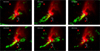 |
Fig. B.2 Continuation of Fig. B.1. |
| In the text | |
|
Fig. C.1 Spectral energy distribution in the mid-IR, submillimeter and millimeter bands in the direction of YSO-G29. The bolometric flux of the region is estimated as the area under the linear interpolation of the fluxes. |
| In the text | |
|
Fig. D.1 Ks Gemini-NIRI image with ALMA continuum at 1.3 mm contours as presented above. The green dashed circle indicates the position from which spectra presented in Figs. D.2 and D.3 were extracted. |
| In the text | |
|
Fig. D.2 Spectra of the eight spectral windows analysed in this study. Panels a), b), e), and f) present data obtained from the observations reported by Liu et al. (Project 2021.1.00311.S), whereas panels c), d), g), and h) correspond to the dataset acquired by Fuller et al. (Project 2015.1.01312.S). Each spectrum was extracted from a beam-size region centred at the peak of the continuum emission. Molecular transitions were identified using the SDAS database. |
| In the text | |
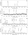 |
Fig. D.3 Continuation of Fig. D.2. |
| In the text | |
|
Fig. D.4 Rotational diagrams of selected molecules towards YSO-G29: (a) CH3CN, (b) HC3N, (c) E − CH3OH, (d) A − CH3OH, (e) CH3OCH3, and (f) CH3CCH. Panels c), d), and f) are reproduced from Martinez et al. (2025, in prep.). The coloured lines represent the best linear fit of each dataset. For HC3N, the uncertainty of the rotational temperature was not estimated due to insufficient degrees of freedom. |
| In the text | |
Current usage metrics show cumulative count of Article Views (full-text article views including HTML views, PDF and ePub downloads, according to the available data) and Abstracts Views on Vision4Press platform.
Data correspond to usage on the plateform after 2015. The current usage metrics is available 48-96 hours after online publication and is updated daily on week days.
Initial download of the metrics may take a while.