| Issue |
A&A
Volume 702, October 2025
|
|
|---|---|---|
| Article Number | A57 | |
| Number of page(s) | 25 | |
| Section | Extragalactic astronomy | |
| DOI | https://doi.org/10.1051/0004-6361/202555816 | |
| Published online | 07 October 2025 | |
RUBIES: A spectroscopic census of little red dots
All point sources with v-shaped continua have broad lines
1
Max-Planck-Institut für Astronomie, Königstuhl 17 D-69117, Heidelberg, Germany
2
Center for Interdisciplinary Exploration and Research in Astrophysics (CIERA), Northwestern University, 1800 Sherman Ave, Evanston, IL 60201, USA
3
Department of Astrophysical Sciences, Princeton University, 4 Ivy Lane, Princeton, NJ 08544, USA
4
Centre for Astrophysics and Supercomputing, Swinburne University of Technology, Melbourne, VIC 3122, Australia
5
Cosmic Dawn Center (DAWN), Copenhagen, Denmark
6
Niels Bohr Institute, University of Copenhagen, Jagtvej 128, Copenhagen, Denmark
7
Department of Physics and Astronomy and PITT PACC, University of Pittsburgh, Pittsburgh, PA 15260, USA
8
Leiden Observatory, Leiden University, PO Box 9513 NL-2300 RA Leiden, The Netherlands
9
Department of Astronomy & Astrophysics; Institute for Computational & Data Sciences; Institute for Gravitation and the Cosmos; The Pennsylvania State University, University Park, PA 16802, USA
10
Department of Astronomy, University of Wisconsin-Madison, Madison, WI 53706, USA
11
Institute of Science and Technology Austria (ISTA), Am Campus 1 3400 Klosterneuburg, Austria
12
MIT Kavli Institute for Astrophysics and Space Research, 70 Vassar Street, Cambridge, MA 02139, USA
13
Department of Astronomy, University of Geneva, Chemin Pegasi 51 1290 Versoix, Switzerland
14
Department of Astronomy, University of Massachusetts, Amherst, MA 01003, USA
15
NSF National Optical-Infrared Astronomy Research Laboratory, 950 North Cherry Avenue, Tucson, AZ 85719, USA
⋆ Corresponding author: This email address is being protected from spambots. You need JavaScript enabled to view it.
Received:
4
June
2025
Accepted:
29
July
2025
Abstract
The physical nature of little red dots (LRDs), a population of compact red galaxies revealed by JWST, remains unclear. Photometric samples were constructed from varying selection criteria with limited spectroscopic follow-up available to test intrinsic spectral shapes and the prevalence of broad emission lines. We used the RUBIES survey, a large spectroscopic program with wide color-morphology coverage and homogeneous data quality, to systematically analyze the emission-line kinematics, spectral shapes, and morphologies of ∼1500 galaxies at z > 3.1. We identified broad Balmer lines via a novel fitting approach that simultaneously models NIRSpec/PRISM and G395M spectra, yielding 80 broad-line sources with 28 (35%) at z > 6. A large subpopulation naturally emerged from the broad Balmer line sources, with 36 exhibiting v-shaped UV-to-optical continua and a dominant point source component in the rest-optical; we define these as spectroscopic LRDs, constituting the largest such sample to date. Strikingly, the spectroscopic LRD population is largely recovered when either a broad line or rest-optical point source is required in combination with a v-shaped continuum, suggesting an inherent link between these three defining characteristics. We compared the spectroscopic LRD sample to published photometric searches. Although these selections have high accuracy, 80%−95% down to F444W < 26.5, only 50%−80% of the RUBIES LRDs were photometrically identified, depending on the selection criteria used. The remainder were missed due to a mixture of faint rest-UV photometry, comparatively blue rest-optical colors, or highly uncertain photometric redshifts. Our findings highlight that well-selected spectroscopic campaigns are essential for robust LRD identification, while photometric criteria require refinement to capture the full population.
Key words: galaxies: active / galaxies: high-redshift
Brinson Prize Fellow.
NHFP NASA Hubble Fellow.
© The Authors 2025
 Open Access article, published by EDP Sciences, under the terms of the Creative Commons Attribution License (https://creativecommons.org/licenses/by/4.0), which permits unrestricted use, distribution, and reproduction in any medium, provided the original work is properly cited.
This article is published in open access under the Subscribe to Open model.
Open access funding provided by Max Planck Society.
1. Introduction
The James Webb Space Telescope (JWST; Gardner et al. 2023) has revealed a remarkable population of high-redshift sources with extremely red rest-optical colors. These sources span a broad redshift range (z ∼ 1 − 10; de Graaff et al. 2025a) and show diverse morphological properties, ranging from unresolved point sources to large disks that extend out to several kiloparsecs (e.g. Baggen et al. 2023; Furtak et al. 2023; Pérez-González et al. 2023; Gibson et al. 2024; Williams et al. 2024; Xiao et al. 2025). Follow-up spectroscopy has revealed a variety of spectral properties. Although high equivalent width emission lines explain the red broadband colors of some sources (e.g., Larson et al. 2023), others indeed have red continua, which can be smoothly rising or show strong spectral breaks (e.g., Carnall et al. 2024; Cooper et al. 2025; Wang et al. 2024). Importantly, this diversity in properties also points to a mixture of physical interpretations, including (dust-reddened) star formation, evolved stellar populations, or emission from active galactic nuclei (AGN).
A peculiar subset of red sources are distinguished by their highly compact nature, and are commonly referred to as little red dots (LRDs). While the term was originally coined by Matthee et al. 2024 to describe potential AGN with broad Balmer emission that appeared red and compact in JWST/NIRCam rest-optical imaging, its usage has since expanded. In particular, several independent searches aimed at identifying extremely massive galaxies within the first gigayear of the Universe relied on NIRCam photometry alone to select candidates based on very red observed rest-optical colors (F277W − F444W ≳ 1), indicative of strong Balmer breaks, along with nondetections at wavelengths shorter than 1 μm, consistent with a Lyman-α break at z ≳ 6 Labbé et al. 2023; Barro et al. 2024. These searches uncovered a population of objects with v-shaped continua: red in the rest-optical, but blue in the rest-UV, many of which also exhibit point-like morphologies in the long-wavelength (LW) NIRCam bands and have since also been referred to as LRDs.
Follow-up spectroscopy with JWST/NIRSpec of individual sources has suggested an intriguing link between compact, red photometric sources and broad-line AGN. The strongly lensed source with a v-shaped broadband spectral energy distribution (SED) of Furtak et al. 2023 was shown to have broad (FWHM ∼ 3000 km s−1) Balmer emission lines consistent with AGN emission Furtak et al. 2024. Among the candidate massive galaxies at zphot ∼ 7 − 9 identified by Labbé et al. 2023, one was spectroscopically confirmed as a broad-line AGN at zspec = 5.6 Kocevski et al. 2023, while others were verified at high redshift and showed both strong Balmer breaks and broad Balmer lines Wang et al. 2024. Greene et al. 2024 conducted the first systematic spectroscopic follow-up of photometric LRDs from Labbe et al. 2025 as part of the UNCOVER survey Bezanson et al. 2024, finding that 9/12 sources (75%) exhibit broad Balmer emission. Collectively, these studies suggest a high incidence of broad-line AGN among some LRD samples, though the exact fraction appears sensitive to the selection criteria and highlights the need for uniform, large-scale spectroscopic follow-up.
If interpreted as AGN-dominated sources, the number density of LRDs would exceed that of the faint AGN expected from extrapolation of the quasar UV luminosity function by an order of magnitude Matthee et al. 2024; Pizzati et al. 2025. Furthermore, if the LRDs were AGN with properties consistent with their lower-redshift counterparts, the implied high black hole masses would appear to greatly exceed local BH-galaxy scaling relations (e.g., Harikane et al. 2023; Maiolino et al. 2024; Furtak et al. 2024; Kokorev et al. 2023), though this may be, in part, due to biases in estimating host properties, AGN attenuation or bolometric luminosities, and/or black-hole masses (e.g., Li et al. 2025; Rusakov et al. 2025; Chen et al. 2025a). The population of LRDs may therefore have important implications for our understanding of the formation and growth history of supermassive black holes.
On the other hand, if the rest-optical continuum is dominated by starlight, it would imply the presence of very massive galaxies in the first gigayear (up to 1011 M⊙ by z ∼ 7 − 8; Labbé et al. 2023), requiring extremely efficient star formation that pushes the boundaries of the maximum stellar mass growth possible in the ΛCDM model Boylan-Kolchin 2023. Combined with their highly compact morphologies, it would also imply that LRDs are the densest stellar systems in the Universe Baggen et al. 2024; Guia et al. 2024; Ma et al. 2025; de Graaff et al. 2025b, exceeding observations and theoretical expectations of the maximum densities in star clusters Hopkins et al. 2010; Grudić et al. 2019. However, this is unlikely to be true for all LRDs, as some show Balmer breaks that are far stronger than can be produced with evolved stars alone de Graaff et al. 2025b; Naidu et al. 2025.
This uncertainty has motivated systematic searches aimed at quantifying the prevalence of LRDs and characterizing their population-wide properties, which so far have focused primarily on photometry (e.g., Labbe et al. 2025; Barro et al. 2024; Kokorev et al. 2024; Kocevski et al. 2025; Pérez-González et al. 2024; Akins et al. 2024). Although the precise selection criterion used differs for each study, all require a red rest-optical continuum, most require that the rest-optical morphology is unresolved or very compact, and some additionally require that the continuum is v-shaped, i.e., a blue rest-UV continuum as well as a red rest-optical continuum. Notably, the inferred number densities and SED properties vary greatly depending on the selection method and modeling choices. Whereas some favor an AGN-dominated interpretation of the SED, using the LRD population to quantify the AGN bolometric, luminosity and/or black hole mass functions (e.g., Labbe et al. 2025; Kocevski et al. 2025; Kokorev et al. 2024), others argue that the SEDs may be best described by stellar populations and that LRDs therefore represent a class of dust-obscured star-forming galaxies Pérez-González et al. 2024 or dust-obscured post-starburst galaxies (e.g., Labbé et al. 2023; Labbe et al. 2024; Williams et al. 2024; Wang et al. 2024, 2025). Hainline et al. 2025 also point out that a large fraction of sources may not have red continua, but that the broadband colors may be boosted by strong emission lines. Finally, brown dwarfs can also appear to have v-shaped broadband photometric SEDs and are necessarily point sources (e.g., Langeroodi & Hjorth 2023; Greene et al. 2024; Hainline et al. 2024, 2025).
Although targeted spectroscopic follow-up of small LRD samples has revealed a high fraction of broad Balmer emission lines and v-shaped continua, it remains unclear how these findings extend to the broader photometric samples in the literature, whose selection criteria can vary significantly. For example, Pérez-González et al. 2024 compiled spectra from various spectroscopic surveys for 18 sources in their photometric LRD sample and found that only 3 show broad Balmer emission, three times fewer than reported in the systematic follow-up by Greene et al. 2024. These discrepancies have critical implications for the interpretation of the physical properties of LRDs.
To robustly link the spectral properties of LRDs to these large photometric samples therefore requires comprehensive follow-up spectroscopy of photometric candidates. The JWST/NIRCam grism has been demonstrated to be highly successful at determining robust redshifts and selecting broad Balmer emission lines (e.g., Matthee et al. 2024; Naidu et al. 2024; Sun et al. 2025; Lin et al. 2024, 2025), but simultaneous coverage of forbidden lines such as [O III] is still rare, making it difficult to rule out broadening from stellar feedback and outflows. Only JWST/NIRSpec can reveal the continuum shape and at the same time kinematically resolve multiple emission lines. However, such targeted follow-up often leads to a complex spectroscopic selection function, and robustly quantifying the fraction of photometrically selected LRDs with broad Balmer lines and v-shaped continua is therefore challenging.
The Red Unknowns: Bright Infrared Extragalactic Survey (RUBIES; de Graaff et al. 2025a) was designed to deliver a large spectroscopic dataset with a well-characterized selection function: RUBIES has observed a large number (∼300) of red sources without morphological pre-selection, while at the same time has sampled several thousand galaxies with a broad distribution in color space. For this paper, we used the full RUBIES dataset at z > 3.1 to robustly quantify the prevalence of (1) broad Balmer emission lines, (2) v-shaped continua, and (3) a dominant point source in the rest-optical. As we show below, a population of spectroscopic LRDs, i.e., those that meet all three criteria, naturally arises from the data, hinting that these features may be physically interlinked.
In Section 2 we present an overview of the RUBIES survey and the relevant data used in this work. We describe our methodology for measuring typical LRD features in Section 3, while in Sect. 4 we explore the relationship between these characteristics to construct a spectroscopic LRD definition. Section 5 compares our results to existing photometric LRD selection techniques. Finally, we present our summary and discussion in Section 6. Where relevant, we assume a flat ΛCDM cosmological model with Ωm = 0.3 and h = 0.7. All magnitudes are reported using the AB system Oke & Gunn 1983 and nondetections (< 1σ) are reported as their 1σ upper limits.
2. Data and spectroscopic sample
The JWST Cycle 2 program RUBIES (GO-4233; PIs: de Graaff & Brammer) is a 60-hour spectroscopic survey with the NIRSpec microshutter array (MSA) that has observed ∼4500 high-redshift sources selected across ∼150 arcmin2 from JWST Cycle 1 NIRCam imaging programs. A detailed description of the observing strategy, parent catalogs, and spectroscopic selection function, as well as the spectroscopic data reduction can be found in de Graaff et al. 2025a. In this section, we provide a brief summary of key details relevant to this work.
2.1. JWST imaging
The RUBIES targets were selected from two extragalactic deep fields, the Ultra Deep Survey (UDS) and Extended Growth Strip (EGS). Both fields have extensive photometric coverage from X-ray to radio wavelengths, and were central to the CANDELS and 3D-HST surveys Grogin et al. 2011; Koekemoer et al. 2011; Brammer et al. 2012; Skelton et al. 2014. Public JWST/NIRCam imaging was obtained for these fields as part of multiple programs in Cycles 1−3.
For the EGS the majority of NIRCam imaging data comes from the Cosmic Evolution Early Release Science Survey (CEERS; GO-1345, PI: Finkelstein; Finkelstein et al. 2025). This imaging spans approximately 80 arcmin2 Bagley et al. 2023 in 7 different NIRCam filters (F115W, F150W, F200W, F277W, F356W, F410M, F444W), with a 5σ point source depth of 28.6 mag at 4 μm. In addition, the Cycle 1 program GO-2234 (PI: Bañados; Khusanova et al., in prep.) obtained NIRCam/F090W imaging over the same footprint as CEERS.
The UDS was one of two fields observed as part of the Public Release IMaging for Extragalactic Research Survey (PRIMER; GO-1837; PI: Dunlop). This survey used the same 8 filters as the programs in the EGS, reaching a comparable typical depth (see Donnan et al. 2024), but for a larger area of ∼220 arcmin2. Combined, these surveys therefore provide a homogeneous dataset for spectroscopic follow-up.
All imaging data were reduced with the grizli pipeline Brammer 2023a, the details of which are described in Valentino et al. 2023. The resulting image mosaics have a pixel scale of 0.04″ and are publicly available from the DAWN JWST Archive1 (DJA). The RUBIES targets were selected using version 7.2 of the DJA image mosaics; for this paper we used version 7.2 for the UDS mosaics and version 7.4 for the EGS mosaics to perform morphological modeling.
The RUBIES photometric parent catalog was constructed primarily from the public catalogs on the DJA, with photometry measured in circular apertures of diameter 0.5″ and photometric redshift measurements from eazy Brammer et al. 2008. This catalog was thoroughly visually inspected to remove artifacts and stars and supplemented with a small number of candidate high-redshift (z > 6.5) sources from the photometric catalogs of Weibel et al. 2024.
We caution that the photometry in this parent catalog does not account for the wavelength-dependent point spread function (PSF) of JWST. To measure consistent colors in this paper, we therefore cross-match our final spectroscopic sample, as described in Section 2.2, to the catalogs of Weibel et al. 2024, who provide photometry measured from image mosaics that were matched in resolution to the F444W filter using empirical PSF models. We use circular aperture flux measurements with diameter of 0.5″ to compute colors, and use the Kron flux measured in the F444W band as a measurement of the total flux.
2.2. RUBIES spectroscopy
The RUBIES dataset consists of 12 NIRSpec MSA pointings in the UDS and 6 pointings in the EGS, covering a total area of approximately 150 arcmin2. The pointing locations were chosen to optimize the total number of high-priority targets across the survey. Priorities were assigned to sources in the parent catalog using a small number of parameters (see de Graaff et al. 2025a for full details): the total flux at 4 μm, F150W−F444W color, and photometric redshift. The highest priority red sources were selected by requiring F444W < 27 and F150W − F444W > 2 with no restriction on photometric redshift; high-priority high-redshift sources were selected by F444W < 27 and zphot > 6.5 with visual vetting to remove low-redshift interlopers. The remainder of the catalog was rank-ordered using the source weight W, a quantity that is inversely proportional to the source number density in the parameter space of F444W, F150W−F444W and zphot. In designing the masks, targets were assigned shutters in order of priority and weight.
In total there are 4444 unique spectroscopic targets. As the result of the prioritization strategy, this sample includes a large number of rare, red sources at z > 1 and the survey overall reaches high spectroscopic completeness (> 70%) in sparsely populated regions in observed color space. Source morphology was explicitly not used in any of the target prioritization, and RUBIES therefore probes a large variation of red sources, ranging from LRDs to dust-obscured extended star-forming disks. At the same time, the survey includes a representative sample of the high-redshift population that is less red, providing a crucial census sample to place rare sources in context.
Of the 4444 targets, approximately 3000 were observed with both the low-resolution PRISM/CLEAR (ℛ ∼ 50 − 500; 0.6 − 5.5 μm) and medium-resolution G395M/F290LP (ℛ ∼ 1000 − 1500; 2.7 − 5.5 μm) disperser/filter combinations. The remainder were observed only with the G395M grating. Observations were taken by constructing 3-shutter slitlets for each target and performing a 3-point nodding pattern. The total exposure time is 48 min for each disperser.
The RUBIES spectra were reduced using version 3 of the msaexp pipeline Brammer 2023b, as described in detail in Heintz et al. 2025 and de Graaff et al. 2025a. These reductions offer two types of background subtraction for the PRISM mode. To ensure that the spectral extractions of the PRISM and G395M spectra are matched, we use only the local background subtracted spectra in this paper, i.e., those obtained from the image differences between the three nodded exposures. Spectroscopic redshifts were measured with the msaexp template fitting and visually inspected to assign quality flags. Grading is fully described in Section 3.2 of de Graaff et al. 2025a; however, we note that a grade = 3 corresponds to a robust redshift. We note that RUBIES overall has a very high spectroscopic success rate, as approximately 90% (70%) of high-priority red sources (all sources) have robust redshifts. We find a total of 2014 sources with robust redshifts and both G395M and PRISM spectroscopy.
For a subset of sources (N = 297), we also use the newly developed version 4 of msaexp (Brammer et al., in prep.). The most important change in version 4 is in the flux calibration, which was re-derived empirically from standard stars observed in a range of commissioning and calibration programs. Crucially, these new calibrations extend the nominal wavelength ranges of the PRISM and G395M dispersers by ±0.2 μm, enabling the measurement of [O III] and Hα emission down to z ∼ 5.5 and z ∼ 3.1 in G395M compared to z ∼ 5.8 and z ∼ 3.4 respectively, and Hα out to z ∼ 7.4 in both dispersers compared to z ∼ 7.1. We use these v4 reductions only for broad-line identification for sources at zspec ∈ [3.1, 3.4] and zspec > 6.9, and rely on the v3 reductions for other analyses, i.e., continuum fitting.
Lastly, we add one serendipitous compact red source (F444W = 24.1) to our sample that was coincidentally observed as the neighbor of a lower-priority object (RUBIES-UDS-50432) in an outer slitlet. Using a custom spectral extraction using the global background, we determine that the source is at zspec = 6.42 and could potentially be a bright LRD as preliminary visual inspections of its spectroscopy indicate a broad line and v-shaped continuum. This source is referred to as RUBIES-UDS-57040 going forward.
To select our final sample for uniform and robust broad line identification, we require a robust zspec, i.e., visually inspected grade = 3, and that either the Hα or Hβ line fall into the G395M defined as any pixels falling within 1000 km s−1 of the emission line position predicted by the DJA zspec. This is especially relevant for robustly detecting broad lines at lower redshifts as the resolution of the PRISM disperser is very low (ℛ < 100) at < 3 μm. In practice, this limits our sample to zspec > 3.1 with the extended coverage from the v4 reduction. This yields a sample of 1482 sources, with a median redshift of zspec = 4.66 and maximum redshift of zspec = 9.3, hereafter referred to as RUBIES sources with robust zspec > 3.1. Of these 1198 (80%) have PRISM spectroscopy; only these targets are used to to measure LRD features in the following sections. As shown in Figures 5 and 6 of de Graaff et al. 2025a, the z ≳ 3 sources in RUBIES have a broad distribution in color space, spanning not only a broad range in the color used for target prioritization, F150W−F444W, but also in F115W−F200W and F277W−F444W.
The diversity of our sample extends far beyond broadband colors. In Figure 1 we demonstrate that sources with similar observed colors can have drastically different spectral shapes, emission line properties, and emission line kinematics. In the top row, we present a prototypical LRD: a point-like red source with a v-shaped continuum and broad Hα emission. The middle row shows a compact, yet resolved, dusty star-forming galaxy, which has a v-shaped continuum but narrow Hα and [N II] emission. The bottom row shows an AGN, a point source with a relatively blue continuum that appears red in broadband photometry due to strong emission lines, including broad Hα emission. Despite similar broadband colors, the sources span a wide range of morphologies, star formation histories, dust content, and ionizing mechanisms. The spectroscopic diversity of these sources underscores the importance of the RUBIES spectroscopic dataset for disentangling the nature of red JWST sources.
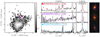 |
Fig. 1. Diversity of red high-redshift sources in RUBIES. Right: F115W−F200W vs. F277W−F444W for RUBIES sources with robust zspec > 3.1 (gray histogram), which populate a broad distribution in color space. Right: PRISM spectra and NIRCam photometry, G395M spectra (zoomed in on Hα), and 1″ × 1″ NIRCam F444W/F277W/F150W RGB images for three RUBIES targets that are close in color space. The top row shows a typical LRD, with a v-shaped continuum, broad Hα emission line and very compact morphology. The middle row shows an extended red object with a v-shaped continuum, but narrow Hα and [N II] emission. The red source in the bottom row is a point source with a relatively blue continuum, but appears as red due to high equivalent width emission lines, including a broad Hα line. This demonstrates that sources with similar broadband photometric colors can have very different spectral properties. |
3. LRD features
In this section we aim to robustly measure photometric and spectroscopic features commonly associated with LRDs: a broad Balmer line in Section 3.1, a v-shaped continuum in Section 3.2, and a dominant rest-optical point source in Section 3.3.
3.1. Broad Balmer emission
Our goal is to robustly identify and measure broad emission components that are distinct from narrow line emission and uniquely associated with the Balmer lines, i.e., Hα and Hβ. This requires differentiating broad Balmer emission from potential contamination by other broadening mechanisms, such as galactic outflows that might similarly affect forbidden lines, for example [O III].
3.1.1. Simultaneous spectroscopic fitting
To impose the strictest constraints on the presence of broad emission lines, we introduce the Python package unite2, Uniform NIRSpec Inference (Turbo) Engine Hviding 2025, to simultaneously fit all available NIRSpec spectra for each individual source within a given mask. Because extractions within a mask are performed using a consistent aperture, background subtraction, and trace extraction, we assume that the intrinsic source spectrum is the same across exposures. Differences between spectra arise primarily from the dispersion characteristics of the gratings, which affect the spectral resolution and sampling, as well as from relative calibration uncertainties between dispersers. By jointly fitting these spectra, we leverage the complementary wavelength coverage, signal-to-noise (S/N), and resolution to enhance our sensitivity to broad emission features. For sources observed in multiple masks, we treat each mask independently, as differing apertures preclude the assumption of a shared underlying spectrum. The mask with the highest S/N spectra is taken as the fiducial mask for a source.
We begin by constructing a statistical model for emission lines and continua: we include the Hα and Hβ emission lines along with the [O III]λλ4960, 5008 Å, [N II]λλ6549, 6585 Å, and [S II]λλ6718, 6732 Å doublets. Our fitting region is centered around each line and extends ±15 000 km s−1. Overlapping regions are merged, resulting in two primary fitting windows: 4619 Å−5258 Å and 6222 Å−7070 Å in the rest frame. Each region is modeled with a linear continuum, where the slope θ follows a noninformative prior, θ ∼ 𝒰(−π/2, π/2), and the height is drawn from a broad uniform prior based on an initial continuum estimate. Emission lines are modeled as Gaussians, with redshift z ∼ 𝒰(zspec − 0.005, zspec + 0.005), FWHM wnarrow ∼ 𝒰(0, 750) km s−1, and flux constrained to be positive, drawn from a broad uniform prior based on an initial flux estimate.
Because the default pipeline does not account for covariance in error propagation, we rescale the error spectrum in each fitting region to account for systematic over- or underestimation of uncertainties. We mask ±3500 km s−1 around each expected emission line to isolate the continuum. The remaining region is fit with a weighted least squares (WLS) linear model from which we compute the reduced chi-squared, χν2. Assuming that the continuum is well described by a linear model, the normalized residuals should have unit variance. To enforce this, we multiply the error spectrum by  in each region and for each disperser. This correction ensures that uncertainties in the final fit reflect the true variance in the continuum, improving the reliability of emission line constraints. Across all RUBIES spectra in this work, we find a typical correction factor of ∼1.1 ± 0.2.
We build two physical models: a narrow model, consisting only of narrow emission lines, and a broad model, which includes additional broad Balmer emission lines. In the narrow model, all emission lines share a common redshift and intrinsic velocity width. The broad model extends this by incorporating two additional Gaussians for Hα and Hβ. To ensure reliable broad line detection, these additional lines are constrained to share the same redshift as the narrow lines. However, their FWHM is drawn from the prior wbroad ∼ 𝒰(wnarrow + 100, 2500) km s−1. For both models, the [O III] and [N II] flux ratios are fixed to the quantum-mechanically derived values of 1:2.98 and 1:2.95 respectively Galavis et al. 1997.
Fitting the physical model to each spectrum requires accounting for several instrumental and observational effects. First, emission lines are broadened by the line-spread function (LSF), using the NIRSpec LSF curves of an idealized point source obtained with msafit de Graaff et al. 2024. Because these are model LSFs rather than empirical calibrations, we introduce a scale factor drawn from a prior, sLSF ∼ 𝒩(1.2, 0.1), truncated to [0.9, 1.5], to adjust for potential deviations. To address systematic flux offsets between the G395M and PRISM spectra observed in de Graaff et al. 2025a, we introduce a flux scale prior. The G395M scale is fixed at 1, while the PRISM scale follows sflux ∼ 𝒩(1.1, 0.2), truncated to [0.5, 1.7], reflecting the observed range. Similarly, we account for pixel offsets between the two dispersers, with the G395M offset fixed at 0 and the PRISM offset drawn from δpx ∼ 𝒰(−0.3, 0.7) px. The choice of G395M as the reference is arbitrary and symmetric, ensuring that the relevant fluxes and redshifts remain recoverable for either disperser. Finally, to account for NIRSpec detector’s undersampling of the LSF, the model is integrated in each pixel, rather than computed at the pixel center, before comparison with the observed data.
We implement these models using NumPyro Phan et al. 2019, a probabilistic programming library built on top of JAX Bradbury et al. 2018. Leveraging JAX’s automatic differentiation and Just-In-Time (JIT) compilation, NumPyro allows us to efficiently define and sample from our joint Bayesian model. We employ Markov chain Monte Carlo (MCMC) using the No-U-Turn Sampler (NUTS; Hoffman & Gelman 2014) with one chain comprised of 250 warmup steps and 500 posterior samples, ensuring robust convergence diagnostics and a typical runtime of < 10 seconds for a typical source. Finally, to compare the relative model fits, we compute the Widely Applicable Information Criterion (WAIC) Watanabe & Opper 2010, which accounts for model complexity while estimating out-of-sample predictive accuracy.
We present an example of our simultaneous broad and narrow fitting for RUBIES-EGS-926125 and RUBIES-EGS-966323 in Figure 2. The latter source was not conclusively identified as a broad-line source in Kocevski et al. 2025, denoted as CEERS-9083, or Wang et al. 2024. Due to the low S/N in the G395M spectrum and the relatively narrow width of the broad component, the broad-line was not identified from single spectrum fitting. By simultaneously leveraging the resolution of the G395M to constrain the narrow line width and the S/N of the PRISM to detect deviations from the derived width, the broad line is measured with a ΔWAIC = 55, i.e., a > 6σ detection.
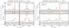 |
Fig. 2. Zoomed-in images of the spectroscopic fits for RUBIES-EGS-926125 (left) and RUBIES-EGS-966323 (right) using narrow (blue) and broad (orange) models for both G395M (top) and PRISM (bottom) spectra along with their residual deviations. We plot the maximum posterior sample from the MCMC fitting. Simultaneous fitting leverages all available data to constrain linewidths in both gratings across different wavelength regimes. For 926125 we show both the Hβ + [O III] and Hα + [N II] complexes, while for 966323 we only have coverage of the Hβ + [O III] complex. We note that a broad component could not be conclusively fit in 966323 from the PRISM or G395M spectrum alone in Wang et al. 2024 or Kocevski et al. 2025, but is detected in this work at the > 6.5σ level. |
3.1.2. Broad line validation
While a broad Balmer line will lead to a better fit with our fitting setup, data quality (DQ) issues can lead to a statistically improved fit even when the line profile is not well described by two kinematic components. An initial examination of the data reveal several failure modes for our unite fits: spectral trace overlaps, low S/N, or large offsets between the PRISM and G395M dispersers. To minimize contamination from false positives, we therefore implement the following quality cuts:
-
A ΔWAIC > 11.8, corresponding to a confidence level greater than 3σ is required, i.e., ensuring that the improvement in fit provided by the broad model is statistically significant over the narrow model alone.
-
wbroad > 1000 km s−1 to exclude narrow-line contamination or ambiguous features.
-
In spectra with both Hα and Hβ coverage, the flux of the broad Hα must exceed the flux of the Hβ in order to eliminate unphysical fits.
Following our quality cuts, three individuals (REH, AdG, JEG) visually inspected all 121 broad-line candidates. The inspectors identified 19 sources (15.7%) with no clear evidence for a broad component (requiring 2/3 agreement), finding these cases showed flux contamination in the G395M due to other traces or DQ artifacts near the edge of the spectral range. We refer to these, and any other fitting failures due to DQ issues as indeterminate broad sources and present the common failure modes in Appendix B. In addition, we also denote objects without Hα coverage and no broad Balmer detection as indeterminate broad sources.
However, a detected broad Balmer line does not guarantee that the line is not due to phenomena that can broaden other narrow lines, such as star-formation-driven outflows. We therefore use information from forbidden transitions, such as [O III], to investigate the origin of the broad line. For nearly every zspec ≳ 5 galaxy we recover [O III] in the G395M grating, provided the line does not fall into a chip gap or encounter other DQ issues. To distinguish between these scenarios, we further refine our sample of 102 detected broad Balmer lines based on the following criteria:
-
wbroad ≥ 1500 km s−1: we attribute the broadening to arise from nonstellar feedback origins and therefore be tied directly to the Balmer line itself (N = 69). While it is not impossible for feedback and outflows to generate velocities in excess of this limit, the number of these outflows even in AGN-driven scenarios, drops sharply beyond 1000 km s−1 Hao et al. 2005; Leung et al. 2019; Förster Schreiber et al. 2019. In addition, we note that we still visually inspect the forbidden-line properties where available for this sample and find no evidence for comparable broadening in these lines.
-
wbroad < 1500 km s−1: we then examine other strong nebular emission lines where available in the G395M grating, such as [N II] or [O III].
-
(a)
If no other narrow lines are detected, typically due to a lack of [N II] paired with redshifts where [O III] falls out of the G395M spectrum (z ≲ 5), the Balmer line is not classified as broad and is also referred to as an indeterminate broad source (N = 19).
-
(b)
If another narrow line is detected and there is equal broadening present in that line and/or significant residuals in its fit, as determined by 2/3 agreement, we do not consider the source to be a broad Balmer line source (N = 3).
-
(c)
If another narrow line is detected and there is no broadening present, then the Balmer line is considered to be broad (N = 11).
-
(a)
We therefore conclude with a robust broad Balmer line sample of 80 galaxies and three with broadening in all narrow lines. The availability of both sensitive PRISM and higher-resolution G395M grating spectra allows for robust broad-line selection, yielding one of the largest sample of broad-line objects to date at z > 4 Harikane et al. 2023; Maiolino et al. 2024; Kocevski et al. 2023; Taylor et al. 2025a; Juodžbalis et al. 2025; Lin et al. 2024, 2025; Zhuang et al. 2025. The broad Balmer line sample is presented in Appendix B, including examples of failures of the fitting due to DQ issues.
Our emission line model, i.e., Gaussian profiles with uniform priors, is optimized for broad-line detection rather than detailed characterization. We caution that the reported FWHM values may not best represent the physical system, especially as LRDs often exhibit extended line wings that may be better modeled with Lorentzian functions Wang et al. 2025; de Graaff et al. 2025b; Naidu et al. 2025; Rusakov et al. 2025; Labbe et al. 2024. Future work will address the full emission-line profile modeling taking these intricacies into account.
3.2. V-shaped continuum
To robustly measure the continuum shape of LRDs, we adapt and extend the fitting method described in Setton et al. 2024 to measure spectral slopes from both PRISM spectroscopy and NIRCam photometry. As established in Setton et al. 2024, the break in LRDs preferentially occurs at the Balmer limit of 3645 Å (H∞) in a sample selected independent of broad-line width. We therefore fix the continuum break location and fit the data on either side of the Balmer limit. For the rest-UV, we fit the range from 1200 Å–H∞, and for the rest-optical, we fit the range from H∞–7000 Å. The continua ranges are fit using a power law of the form  with nonlinear least squares optimization.
3.2.1. Photometric continuum
We measure the continuum slopes from photometry by using all available wide NIRCam photometric bands whose central wavelength lie within the aforementioned spectral ranges. In addition, in order to fit a slope we require at least two photometric filters be available in the given spectral range. Since our primary goal in this section is to characterize the intrinsic continuum shape, we only measure photometric continua for sources with accompanying PRISM spectroscopy.
3.2.2. Spectroscopic continuum
In order to mitigate the effect of strong emission lines, we mask the rest-frame spectrum ±50 Å around the Hα, Hβ, Hγ, Hδ, He Iλλ4471, 6680 Å, [O II], and [Ne III] lines along with the [O III] and [N II] doublets. In addition, we require at least 25 wavelength elements be present after applying the emission line mask to fit a slope. While the photometric and spectroscopic continuum fits are performed independently, we use the photometry as evidence for blue rest-UV slopes as the rest-UV faintness or slit losses can lead to low continuum sensitivity. However, we always require a measurement of the rest-optical continuum from the spectroscopy. To define a source as v-shaped from spectroscopy, we impose the following criteria:
-
A blue rest-UV continuum with a nonnegative fit: βUV < −0.2 detected at the 2σ level and aUV > 0 from either spectroscopy or photometry.
-
A red rest-optical continuum with a nonnegative fit: βopt (Spec.) > 0 detected at the 2σ level and aopt (Spec.) > 0.
-
βopt − βUV > 0.5 using the rest-UV slope from spectroscopy if it satisfies our blue rest-UV continuum cut in spectroscopy, otherwise from photometry.
We are able to measure spectroscopic continua in 1158 (97%) of our robust zspec > 3.1 sample with PRISM spectroscopy; of these 55 (5%) are classified as v-shaped.
In Figure 3, we present the continuum fits for RUBIES-EGS-49140 and RUBIES-UDS-934230 using both photometric and spectroscopic data. Although both methods fit the data well, they differ in their results. While the photometry is often able to provide a higher S/N measurement, particularly in the rest-UV, it is significantly impacted by emission line contamination in broadband photometry, leading to different inferred red-optical slopes. However, photometry also can find bluer rest-UV slopes due to the extended UV ‘fluff’ often seen in LRDs Labbe et al. 2024; Rinaldi et al. 2024; Chen et al. 2025b, which can be lost in spectroscopy due to slit losses.
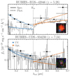 |
Fig. 3. Rest-UV (blue) and rest-optical (orange) continuum fitting of RUBIES-EGS-42046 (top) and RUBIES-UDS-934230 (bottom) from PRISM spectroscopy (solid) and NIRCam photometry (dashed). In the insets are the 0.5″ × 0.5″ NIRCam F444W/F277W/F150W RGB cutouts of the sources. We emphasize that spectroscopic rest-optical continuum fitting can mitigate the effect of strong emission lines, but can suffer in S/N in the rest-UV where the spectrum is fainter or cannot capture extended rest-UV emission due to slit losses. RUBIES-EGS-42046 is identified as a spectroscopic v-shape, while RUBIES-UDS-934230 is not despite a red photometric rest-optical color. |
3.3. Rest-optical point source morphology
Our morphological analysis addresses two key questions: (1) Is the source spatially resolved? and (2) if resolved, is there still a dominant point source component? We first assess basic resolvability in Section 3.3.1, recognizing that Sérsic profile fitting inherently assumes extended emission and requires careful calibration against known point sources. In addition, Section 3.3.2 will investigate whether resolved sources still contain a dominant nuclear point source component.
We characterize unresolved sources by performing Sérsic profile fits using pysersic Pasha & Miller 2023 on all LW NIRCam bands, employing empirical PSFs from Weibel et al. 2024 for convolution. Our analysis requires S/N > 10 per filter and adopts uniform priors for the Sérsic index, n ∼ 𝒰(0.65, 6), and effective radius, reff ∼ 𝒰(0.25, 25) px. The posterior distributions for the morphological parameters are sampled using the NUTS sampler implemented in NumPyro using 2 chains with 1000 warm up and 1000 sampling steps each. We validate fits by requiring  , minimum effective sample size of 250 across all parameters, and χ2/(# px) < 2 to rule out poor sampling or large residuals.
3.3.1. Rest-optical unresolved morphology
We first begin by assessing if the source is spatially resolved at all, i.e., can we robustly detect spatially extended emission beyond the PSF? However, this is not straightforward from Sérsic profile fitting, which by definition assumes an extended profile. Even when a source’s inferred radius approaches the lower bound of the prior, this reflects an imposed modeling choice. While the prior limit can be adjusted, the interpretation ultimately depends on the precision of the PSF model, and there is no definite threshold for declaring a source resolved. We therefore perform Sérsic profiles to our robust zspec > 3.1 sample and a sample of stars which are known point sources and thus unresolved.
We begin by selecting a sample of stars in the UDS field starting with the same criteria used in Weibel et al. 2024 but extending down to fainter magnitudes, 23 < mF444W < 27, to better match the brightness of sources discussed in this study. To eliminate contaminants from this selection, typically compact galaxies at 1 < z < 4, we require that stars satisfy two additional color cuts: F200W − F444W < 0.75 and F150W − F200W < 0.1. Visual inspection of the images and SEDs confirms that these cuts yield a clean sample of stars. We ultimately identify 97 stars, to which we apply the same morphological fitting procedure and S/N cuts as used for our galaxy sample.
The posterior distributions of reff for the stellar sample are all bounded by the lower limit of the prior, with peaks in the distribution near 0.25 px and an extended tail out to larger radii. To quantify the spread of these posteriors, we plot the stellar magnitude against the 95th percentile of the reff posterior, reff, 95%, for each LW NIRCam filter in Figure 4. For bright stars, we observe a floor in reff, 95% around 1/3 px, which we interpret as a systematic limit set by the PSF width and the accuracy of our PSF model. At magnitudes fainter than 25, reff, 95% increases, likely due to lower signal-to-noise ratios broadening the morphological posteriors. We observe that the slope of this increase is approximately 0.2 mag per log(r/px), consistent with a  dependence, confirming our expectation that the trend is driven by Poisson-dominated noise in the source centers.
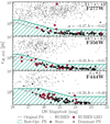 |
Fig. 4. Stellar locus and morphological classification in LW NIRCam filters. The black stars show the 95th percentile effective radius posterior (reff, 95%) vs. magnitude for reference stars, with the best-fit stellar locus (gray dashed line). We classify galaxies as point sources (green hashed area) if they fall below the +4σresid offset of this relation (rrsv; green line). The gray circles show all RUBIES sources with robust zspec > 3.1, red hexagons highlight spectroscopic LRDs (Section 4.2), and black circles mark non-LRD sources with dominant point-sources (Section 3.3.1), plotted in the LW filter that traces the rest-5500 Å flux. |
We use the behavior of stellar magnitude versus reff, 95% to determine whether sources in our sample are spatially resolved. If a source falls within the locus defined by the stars, we classify it as unresolved. To assess this quantitatively, we fit a parametric model to the stellar distribution, described by a power-law with a plateau:
where a and b are the parameters which are optimized separately for each filter. To ensure the curve fully encloses the stellar population, we compute the standard deviation of the residuals from the initial fit, shift both parameters upward by +4σresid, and impose an upper limit of 1.5 px., resulting in curve we denote as rrsv(m). The resulting curve, along with the best-fit a and b values for each filter, is shown in Figure 4.
This analysis reveals the tradeoff in point-source selection: our conservative morphological cut, i.e., imposing a strict 1.5 px upper limit, prioritizes sample accuracy at the potential cost of completeness. While effectively minimizing contamination from compact galaxies, this approach may exclude genuine point sources below ∼26 mag in F444W and ∼27.5 mag in F277W/F356W, where the stellar locus continues to rise beyond our size cutoff (Figure 4). We discuss the impact of this accuracy-completeness tradeoff on point-source selection in Section 5.2.
For each source in our sample we select the LW filter based on the redshift to ensure that the filter probes the rest-optical continuum around ∼5500 Å, i.e., F277W at 3.1 < zspec < 4.6, F356W at 4.6 ≤ zspec < 6.1, and F444W at zspec ≥ 6.1. A galaxy of magnitude m in the relevant filter is then classified as unresolved if reff, 95% < rrsv(m). After removing bad fits and objects which are too faint in the given LW band to confidently measure, we are able to classify the morphologies for 1305 (88%) of our robust zspec > 3.1 sample; of these 1199 (92%) are identified as resolved, while the remaining 106 (8%) are considered unresolved.
3.3.2. Dominant point source component
For sources classified as resolved in Section 3.3.1, we investigate whether they still contain a dominant point-source component in their rest-optical emission. This analysis is particularly relevant for understanding systems where an unresolved nucleus might coexist with extended host emission. However, decomposing these components is inherently challenging due to model dependencies and prior choices. We therefore restrict this analysis to sources that already show either broad Balmer lines or v-shaped continua (N = 32).
We perform two-component modeling using pysersic, fitting each source with a combination of a point source and a Sérsic profile. This largely follows the same procedure for the Sérsic profile fitting above, but we tie the central positions of the two components and add an additional parameter fps, the fraction of flux in the point source component, with a uniform prior; 𝒰(0, 1). We classify a source as having a dominant point source if the 95th percentile of the point-source flux fraction exceeds 50% in the relevant LW filter. We find nine resolved objects with a dominant rest-optical point source: RUBIES-EGS-15825, RUBIES-UDS-23438, RUBIES-UDS-24447, RUBIES-EGS-28812, RUBIES-UDS-33938, RUBIES-EGS-46724, RUBIES-UDS-57040, RUBIES-UDS-167741, and RUBIES-UDS-840721. All nine show broad lines, perhaps unsurprisingly, as a broad Balmer line is a strong indicator of a bright central component. Of these five are also v-shaped.
4. Spectroscopic LRD selection
Following Section 3, we are able to make a confident measurement for all three key characteristics of LRDs in 1019 RUBIES galaxies, i.e., the majority (69%) of our robust zspec > 3.1 sample (85% for the sample with PRISM spectroscopy). We can therefore robustly assess, for the first time, how the combination of a v-shaped continuum, a dominant point-source in the rest-optical, and a broad-line detection correlate among the high-redshift galaxy population.
4.1. Colors and intrinsic spectral slopes
In Figure 5 we plot the color-color distribution of our zspec > 3.1 sample and those that satisfy our condition for broad-line, unresolved, and v-shaped features. We divide the sample into two redshift bins, z < 5 and z ≥ 5, and show NIRCam broadband colors that approximately probe rest-UV versus rest-optical colors in these regimes (F090W−F150W vs. F200W−F356W and F115W−F200W vs. F277W−F444W, respectively). We note that the difference in sample size between the two redshift bins is, in part, driven by the fact that the [O III] doublet is observed in the G395M grating for z > 5, which enables broad line identification down to smaller widths. However, broadband colors can be significantly impacted by emission line contamination, which depends on the spectroscopic redshift and the exact position of the emission line. We therefore show the corresponding intrinsic spectral slopes (βUV vs. βopt) as derived from spectroscopy in Figure 6 to compare and contrast the distributions.
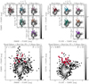 |
Fig. 5. Color-color space distribution of RUBIES sources with robust zspec > 3.1 (gray histogram). We divide the sample into zspec < 5 (right) and zspec > 5 (left) and show the NIRCam F090W−F150W vs. F200W−F356W and F115W−F200W vs. F277W−F444W, respectively, which approximately probe rest-UV vs. rest-optical colors. In the top row we plot objects that satisfy our condition for broad-line, unresolved, and v-shaped features, along with their combinations, above the full distributions of the parent sample in each redshift regime. In the bottom row we plot the objects that satisfy all three criteria. Each panel includes the total number of objects shown and the fraction of the represented sample. The points are colored as in Figure 7. |
4.1.1. Broad Balmer lines
We begin by investigating the observed colors and intrinsic slopes of the full sample with robustly detected broad Balmer emission. Broad-line sources tend to be redder in the rest-optical than the full spectroscopic sample, partly due to luminous broad Hα emission, which can bias rest-optical colors by up to 0.8 mag. In contrast, when comparing to spectral slopes, we find that the broad-line sample spans wider range of rest-optical slopes. Their rest-UV slopes avoid the very reddest rest-UV tail, a region dominated by dusty star-forming galaxies.
4.1.2. Rest-optical point sources
Galaxies that are unresolved or dominated by a point source at rest-optical wavelengths are distributed across much of color space. Again we see a preference for redder rest-optical colors compared to the full sample, although this may be in part due to the S/N criterion used to measure morphologies, i.e., that the rest-optical flux S/N > 10 (see Section 3.3). Similarly, when investigating spectral slopes, unresolved galaxies span the entirety of spectral-slope space populated by the sample, except for the reddest rest-UV slopes where the population is dominated by dusty star-forming galaxies that are typically larger in size.
4.1.3. Spectroscopic v-shaped continuum
Enforcing a spectroscopic v-shaped selection will, by definition, restrict the sample to a limited area of spectral slope space. Similarly, v-shaped objects occupy a limited region of color space, but with slightly more scatter, attributable to emission line boosting, a moving break location that depends on the true source redshift, and low S/N in the bluest filters for the reddest sources. Roughly four-fifths of the v-shaped sources are unresolved. The remaining fifth may be related to the population of dusty starbursts with v-shaped continua and ALMA 1.2 mm detections from Labbe et al. 2025. Many of these galaxies in our sample, while resolved, are compact and show hallmarks of star formation, including strong but narrow Hα and [N II], and may be related to other populations of compact, red, dusty, star-forming galaxies studied with JWST (e.g., Akins et al. 2023; Williams et al. 2024; Pérez-González et al. 2024; Barro et al. 2024).
4.2. Relationship between typical LRD features
We investigate how the full sample of galaxies with broad Balmer lines maps onto the v-shape and morphology selections. We find that the broad-line population divides into roughly three groups:
-
Resolved systems with broad lines. These span a variety of intrinsic slopes and likely represent galaxies with a nondominant AGN.
-
Unresolved systems with broad lines having blue rest-optical and rest-UV slopes that are likely comprised of typical AGN-dominated systems.
-
Broad-line systems with v-shaped continua that are spatially unresolved.
Figure 7 presents the Euler diagram exploring the relationship between all three features. Most remarkably, we find that if one starts with all sources having a v-shaped continuum, then either an unresolved rest-optical morphology or a broad-line selection will yield predominantly objects where all three features are robustly detected (> 80%; red intersection). The remaining ∼20% that do not satisfy the third criterion are overwhelmingly candidate LRDs rather than interlopers from distinctly different populations.
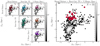 |
Fig. 6. βUV − βopt space distribution of RUBIES sources with robust zspec > 3.1 (gray histogram). On the right, we plot objects that satisfy our condition for broad-line, unresolved, and v-shaped features, along with their combinations, above the full distributions of the parent sample. On the left, we plot the objects that satisfy all three criteria. The slopes are derived from PRISM spectroscopy and each panel includes the total number of objects plotted and their fraction of the represented sample. The points are colored as in Figure 7. |
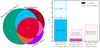 |
Fig. 7. Left: Euler diagram displaying the overlap between the three LRD characteristic criteria: a broad Balmer line, a dominant point source component at rest-optical wavelengths, and a spectroscopic v-shaped continuum. Right: Histogram showing the composition of overlaps in the Euler diagram where only two of the three features are measured. We note that objects with a rest-optical point source and a v-shaped continuum are 80% likely to have a broad line. In fact, in the remaining 20% we cannot reject a broad line, but our quality cuts restrict us from being fully confident. This suggests an underpinning physical link between the three LRD features. |
Specifically, while seven of the v-shaped rest-optical point sources (i.e., the orange intersection) technically lack a broad line detection, they are all classified as indeterminate broad lines, i.e., all are cases with data limitations where the presence of a broad line is ambiguous due to a DQ issue or a lack of coverage of the forbidden lines. Similarly, of the v-shaped with broad-line sources (pink intersection), we find they are all well-described by an additional point-source component, but that the prominence of this component falls below the strict limit (> 50%) we require in this work. We note that one out of five sources, RUBIES-UDS-5496, shows strong [N II] emission not seen in any of our spectroscopic LRDs, as defined in Section 4.2. We assert that this is likely a dusty, star-forming galaxy hosting an AGN and not consistent with the population of spectroscopic LRDs explored in this work.
4.3. A spectroscopic definition of LRDs
We find that all intrinsically v-shaped spectra with dominant point sources in rest-optical imaging exhibit broad Balmer lines, provided the data quality permits their identification. This conclusion arises from a systematic analysis across galaxy color, morphology, and spectral shape, made possible by the RUBIES selection. Moving forward, we define a spectroscopic LRD as a source that simultaneously satisfies these three criteria: a broad Balmer line, a v-shaped continuum, and a dominant point source component in rest-optical imaging. Applying these criteria, we identify 36 spectroscopic LRDs in the RUBIES dataset, the largest such spectroscopic sample to date. NIRCam imaging, PRISM and G395M spectra, and broad line fits for these sources are provided in Appendix A. In addition, we identify seven v-shaped, rest-optical point sources for which broad lines could not be definitively confirmed. Although we consider it plausible that these sources are also spectroscopic LRDs, we do not include them in our spectroscopic LRD sample as DQ issues prevent the definitive measure of a broad Balmer line. These objects are nonetheless presented in Appendix A for completeness.
We briefly investigate how the properties of spectroscopic LRDs compare to the broad Balmer line sources and the robust zspec > 3.1 RUBIES sample. The left panel of Figure 8 demonstrates a wide redshift distribution for the broad-line objects, with the LRDs spanning a similar range in both redshift and rest-optical magnitude. However, it is clear that LRDs are comprised of a distinct family of properties. Typical AGN, with broad lines and blue power-law continua, separate themselves primarily in continuum shape from the LRDs recovered in this work.
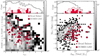 |
Fig. 8. Left: Redshift vs. NIRCam F356W (for zspec ≤ 5) or F444W (for zspec > 5). Right: Absolute UV magnitude (MUV) at 1500 Å, derived from rest-UV spectroscopic slopes, is plotted against total, narrow plus broad, Hα luminosity. RUBIES sources with robust zspec > 3.1 are shown as a gray histogram. Broad-line sources are indicated with dark red circles, and LRDs, defined as galaxies with v-shaped continua, broad Balmer lines, and dominant rest-optical point sources, are shown as light red hexagons. At fixed LHα, LRDs are faint in the rest-UV compared to the full population. Conversely, extreme Hα emitters (LHα ≳ 1010 M⊙) are dominated by LRDs, i.e., LRDs constitute the most luminous Hα emitters at fixed UV luminosity. |
To further highlight their discrepancies, we compute UV luminosities at 1500 Å using the rest-UV continuum fits to the spectra from Section 3.2. In the right panel of Figure 8 we show the total, narrow plus broad, Hα luminosity versus MUV for the full robust zspec > 3.1 sample, the broad Balmer line sources, and the LRD sample. Although both the broad Balmer line sources and LRDs are offset from the bulk of the population, LRDs are the most Hα luminous sources at all MUV. However, the LRDs also show a wide diversity of UV-to-optical ratios, exceeding the much narrower range in LHα at fixed MUV spanned by the typical broad-line sources. We defer a full exploration of the interconnectedness of LRD properties and a physical interpretation to future work.
Overall, we conclude that LRDs – when selected using spectroscopy – comprise a distinct family of properties. Standard broad Balmer sources with power-law continua are well-represented in our sample, but are distinct in both continuum shape and Hα/UV luminosity from the spectroscopic LRDs.
5. Photometric LRD selection
Using an empirical approach to the RUBIES spectroscopic dataset, we have identified a population of LRDs that have broad Balmer emission lines, v-shaped continua, and compact rest-optical morphologies. This is in contrast to typical LRD searches that, to date, have often been based on photometry alone (e.g., Barro et al. 2024; Labbe et al. 2025; Kocevski et al. 2025; Kokorev et al. 2024; Akins et al. 2024). This raises the major question of whether photometric selection of LRDs yields the same sources as our spectroscopic selection. Greene et al. 2024 showed that ≈80% of photometric LRDs from the selection of Labbe et al. 2025 indeed have broad lines and v-shaped continua, albeit from a small sample of 12 sources.
In this section, we use our large spectroscopic sample of LRDs to evaluate the accuracy and completeness rates of popular photometric LRD selection strategies. We then investigate both contaminants and missed LRDs in the photometric samples.
5.1. Broad-line and LRD success rates
Two primary methods have been used to select LRD candidates in photometric surveys. The first is based on identification of v-shaped broadband photometric SEDs, and the second on the selection of red broadband rest-optical colors, sometimes additionally requiring blue rest-UV colors. All methods impose an additional compactness criterion. These different approaches have also been applied in the RUBIES parent fields, EGS and UDS, by three major photometric studies: Kocevski et al. 2025, which used a V-shape selection, and Kokorev et al. 2024 and Barro et al. 2024, which both employed multi-color selection; this provides an ideal opportunity to assess the effectiveness of each method. To quantify the success rates of these photometric methods we cross-match our spectroscopic sample with the public photometric catalogs from each study.
We begin with the selection of Kocevski et al. 2025, which performed double power-law fitting to HST and NIRCam photometry to select v-shaped SEDs. The exact filters used depend on the photometric redshift, but typically comprise three broadband filters both blue- and redward of the estimated Balmer limit. We identify 53 sources with matches to the RUBIES spectroscopy, 47 of which have robust zspec > 3.1. The majority (65%) of these sources show broad Balmer emission lines, in line with an early estimate of the broad line fraction by Kocevski et al. 2025 that was based on a small fraction of the RUBIES dataset. Of the remaining 35%, two thirds are fainter sources where the presence of a broad line cannot be ruled out with the depth of the existing data, while the remainder suffer from data quality issues or lack G395M coverage of forbidden or Balmer lines.
This photometric sample spans a wide range in F444W magnitudes, and nearly half the sample is fainter than the RUBIES LRDs. For a representative analysis of the spectroscopic LRD recovery, we restrict our further comparison to sources brighter than F444W < 26.5. This limit is chosen based on the depth of the RUBIES PRISM spectra, corresponding to a median S/N ∼ 3 per resolution element for a well-centered point source (see de Graaff et al. 2025a). Correspondingly, we find that our v-shape selection is limited to similar magnitudes, where the PRISM spectra provide sufficient S/N for reliable continuum slope measurements. This magnitude limit also broadly applies to our broad-line detection method (see Table 1), though the effective limit in that case depends on additional factors such as line width, equivalent width, and the presence of narrow-line tracers like [O III]. This magnitude threshold thus sets a practical limit on the v-shape selection, and fainter LRDs–particularly those with broad or indeterminate lines–may remain underrepresented in our sample due to insufficient spectral sensitivity. Moreover, as described in Section 3.3.1 and shown in Figure 4, the distinction between genuine point sources and compact galaxies becomes increasingly ambiguous at these fainter magnitudes. We find that 21 of the total 34 spectroscopic LRDs satisfying this magnitude criterion are recovered by the selection of Kocevski et al. 2025. This translates to a success rate, i.e., a spectroscopic LRD completeness, of approximately 60%. We summarize these results in Table 1.
Photometric LRD selection comparison.
Next, we turn to the color-selected sample of Kokorev et al. 2024 which requires two red broadband colors at ∼2 − 4 μm as well as a single blue broadband color at < 2 μm. Although photometric redshifts are not explicitly used, in practice these criteria translate to, and were optimized for, selection on rest-UV and rest-optical colors of high-redshift sources. We find 40 unique cross-matched sources, with 32 having robust zspec > 3.1. This sample contains a remarkably high fraction of broad-line sources, 81%, corroborating the earlier finding of Greene et al. 2024 who evaluated the multi-color selection of Labbe et al. 2025 that is similar to that of Kokorev et al. 2024. The majority of the remaining 19% have indeterminate broad Balmer lines, i.e., lacking G395M coverage of either [O III] or Hα, or suffer from DQ issues, and the true broad line fraction may therefore be even higher. We find that 17 of the 34 RUBIES LRDs at F444W < 26.5 are recovered, which implies a spectroscopic LRD completeness of 50%.
Barro et al. 2024 apply a multi-color selection defined using the F115W, F200W, and F444W bands. These color criteria are informed by the redshifted tracks of a sample of five LRD SEDs spanning z = 3 − 9. Based on a catalog of 440 sources in the UDS and EGS that satisfy the criteria (Barro G., private communication) we find 101 unique cross-matched sources, 84 of which have zspec > 3.1. The confirmed broad-line fraction, 60%, is lower than the other selection methods discussed so far. While this is primarily driven by faint, F444W < 26.5, or indeterminate broad sources, Barro et al. 2024 also selects four sources above our magnitude limit without data quality issues and full availability of relevant emission lines where we are unable to detect broad lines, including the z ∼ 7 quiescent galaxy from Weibel et al. 2025, RUBIES-UDS-977881. This selection recovers the largest number of LRDs among the methods evaluated, identifying 28 of the 34 RUBIES sources in the magnitude-limited sample, corresponding to a completeness of 82%.
Finally, several studies have proposed the use of a single, extremely red rest-optical color to select LRDs (e.g., Akins et al. 2024; Barro et al. 2024; Greene et al. 2024). Multi-color selection has clear advantages, but it relies on the availability of a large number of photometric filters, which do not exist for the widest-area JWST programs such as COSMOS-Web or pure-parallel programs (e.g., Casey et al. 2023; Williams et al. 2025). Although not used before in the RUBIES fields, we also assess the use of the F277W−F444W color paired with our requirement of a dominant rest-optical point source (see Section 3.3). Following Akins et al. 2024, we first impose F277W − F444W > 1.5; due to the restrictive nature of this requirement it selects far fewer galaxies (29, of which 21 have robust zspec > 3.1). The broad line fraction among this sample is very high (78%; see Table 1); however, the recovery of spectroscopic LRDs is highly incomplete (38%) and the single-color selection thus performs significantly worse than the other photometric selections. If the color criterion is instead relaxed to F277W − F444W > 1.0 the LRD completeness improves (67%), but at the expense of the recovered broad line fraction, which drops to 64%.
5.2. Accuracy and contamination
The different photometric LRD selections are all successful in selecting sources with broad Balmer lines (upward of 65−80%), and select a large number of spectroscopic LRDs. This is perhaps not surprising in the context of our results of Section 4, where we demonstrated that a compact rest-optical morphology and v-shaped continuum are highly predictive of the presence of a broad line. However, unlike the spectroscopic v-shape measurements, the photometric colors and v-shapes can be biased by strong emission lines that substantially boost even broadband filters. So far, we have only focused on the success rates of broad line and LRD recovery. We now turn to the contaminants in these samples and the accuracy of the photometric selections.
To investigate the possible contaminants in the photometric samples, we first restrict our analysis to the magnitude-limited sample (F444W < 26.5). Whereas initial follow-up studies of LRDs highlighted brown dwarf stars in the Milky Way as possible interlopers (e.g., Langeroodi & Hjorth 2023; Burgasser et al. 2024; Greene et al. 2024), we find no such contaminants in the photometric samples, demonstrating the success of the color cuts that were imposed to filter out cool stars. In fact, even when expanding to the full sample we only find one faint brown dwarf in the sample selected by Kokorev et al. 2024 and Barro et al. 2024. The other likely class of contaminants consists of AGN or star-forming galaxies with high equivalent width emission lines, which bias the observed rest-optical colors measured from photometry, as demonstrated by Kocevski et al. 2023; Hainline et al. 2025, for example. However, we only identify one or two such sources in the magnitude-limited photometric samples, which are broad-line AGN with blue spectroscopic continua but very strong emission lines.
The sources for which we can confidently conclude that they are LRDs or contaminants therefore account for ∼65% and ∼5%, respectively, of the magnitude-limited photometric selections (see Table 1 and left panel of Figure 9). This still leaves a substantial fraction of sources of uncertain nature, which can be in equal parts ascribed to data quality issues preventing a robust broad-line measurement (e.g., chip gaps, lack of forbidden lines), and low-continuum S/N limiting a robust conclusion on whether the continuum is indeed v-shaped. To define the accuracy of the photometric LRD selections we therefore only consider the sources for which we can robustly determine both the broad line and continuum shape criteria. This spectroscopic LRD accuracy is very high (∼90−95%) for the Kocevski et al. 2025, Kokorev et al. 2024, and single-color photometric selections (as discussed in Section 5.1) and would still be high (∼80%) even in the extreme case that all uncertain sources without data quality issues are considered contamination. The Barro et al. 2024 sample, while more complete than the aforementioned selections, has a lower overall spectroscopic LRD accuracy of 80% with similar contaminants, i.e., blue broad-line AGN, as well as high-z quiescent galaxies, such as RUBIES-UDS-977881 from Weibel et al. 2025.
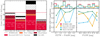 |
Fig. 9. Breakdown of photometric LRD selection methods at F444W < 26.5. The left panel shows how photometric LRDs are distributed among spectroscopically classified categories: spectroscopic LRDs (red), rest-optical point sources and v-shaped galaxies (orange), broad Balmer line sources (dark red), non-LRDs (black), and galaxies with unreliable feature measurements (gray hatched). Overall, photometric LRD selections are accurate but incomplete relative to spectroscopic identifications. The right panel investigates the completeness of the RUBIES photometric LRDs as a function of F277W−F444W color (left) and F115W magnitude (right). The top plots show histograms of RUBIES LRDs (red), matched LRDs from Kocevski et al. (2025, orange), and Kokorev et al. (2024, blue). The bottom plots display the binned completeness of each selection method relative to the RUBIES sample. We find that Kocevski et al. 2025 is incomplete at bluer colors, while Kokorev et al. 2024 is primarily incomplete at fainter rest-UV magnitudes. |
Although the accuracy of the photometric LRD selection is very high, we emphasize that it only applies to the magnitude-limited sample of F444W < 26.5, and it is as of yet unclear how this would extend to the fainter LRD candidates. For these fainter candidates we may expect low-mass star-forming galaxies, i.e., compact sources with strong emission lines, to form a more prominent source of contamination. This is difficult to confirm or rule out with present data, as deep low- and medium-resolution spectra are needed to determine the broad-line and continuum properties. Perhaps even more challenging is the fact that lower-mass galaxies are increasingly compact and therefore difficult to distinguish from true point sources. This effect is especially pronounced in the F444W filter where, at the available depths in the UDS and EGS, the morphological classification must either become inaccurate or incomplete at F444W > 26.5 based on our fits to foreground stars.
5.3. Incompleteness
Most surprising is the fact that the photometric LRD selections are only able to recover up to 60% of the spectroscopic LRDs, even when restricting to F444W < 26.5. This high incompleteness impacts, for example, the inferred number densities and luminosity functions (e.g., Kocevski et al. 2025; Kokorev et al. 2024), and further increases the suggested tension between the inferred black hole properties and theoretical galaxy formation models (e.g., Habouzit 2025).
We investigate the origin of this incompleteness in the photometric samples in the right panel of Figure 9, which shows the spectroscopic LRD completeness as a function of the broadband color F277W−F444W, a proxy for the rest-optical slope, and the F115W magnitude, tracing the rest-UV brightness. This enables us to identify the trade-offs made in each selection method and its impact on LRD completeness. The photometric v-shape selection of Kocevski et al. 2025 requires a strongly rising red rest-optical continuum, and additionally filters out sources that are likely to have strong emission lines based on the F277W−F356W and F277W−F410M colors. As a result, we find that the photometric v-shape selection of Kocevski et al. 2025 becomes increasingly incomplete toward bluer rest-optical colors. Relaxing the rest-optical color criteria would likely improve the completeness, but also would allow more extreme emission line galaxies with intrinsically blue continua to enter the sample. The multi-color selection of Kokorev et al. 2024 allows for more modest rest-optical colors, and the completeness is therefore approximately even across a wide range F277W−F444W color. However, Kokorev et al. 2024 imposed strict S/N criteria on the rest-UV (∼1 − 2 μm) magnitudes, which translates into an incompleteness predominantly at fainter rest-UV magnitudes. Lowering this rest-UV brightness threshold would likely increase the risk of contamination from red interlopers, such as brown dwarfs and compact dusty star-forming galaxies at lower redshifts.
Because these selection methods are incomplete in different regimes, it raises the question whether their combination would yield an improved sample. Indeed, we find only a modest overlap of 11 RUBIES LRDs between the Kocevski et al. 2025 and Kokorev et al. 2024 samples. The combination of the two samples therefore recovers 27 out of 34 spectroscopic LRDs in the magnitude limited sample, corresponding to a joint completeness of 79%. This high completeness is consistent with the findings of Barro et al. 2024, who showed that while the Kocevski et al. 2025 and Kokorev et al. 2024 selections overlap by only ∼50%, the Barro et al. 2024 method recovers nearly all sources selected by both. Our results confirm that this approach achieves broad recovery of spectroscopic LRDs with a completeness of 82% albeit at a compromised accuracy of 80%.
Nevertheless, a substantial fraction of the RUBIES LRDs remains unrecovered by all photometric selection methods. Our analysis has, thus far, neglected one crucial component that spectroscopy provides over photometry: robust redshifts. Redshift is used explicitly in the v-shape fitting of Kocevski et al. 2025 and implicitly enters the color selections of Kokorev et al. 2024 and Barro et al. 2024. These selections may therefore be influenced by uncertainties or systematics in photometric redshift estimation.
We evaluate the photometric redshift success for the robust zspec > 3.1 and spectroscopic LRD samples in the left panel of Figure 10. The reddest sources in RUBIES were selected without any initial photometric redshift constraint and therefore provide an ideal comparison sample. The photometric redshifts were obtained from template fitting to the cross-matched PSF-matched photometry from Weibel et al. 2024 with eazy Brammer et al. 2008, using the blue_sfhz_13 template set. Statistics are performed on the photometric redshift deviation: Δ = |Δz|/(1 + zspec). We find that the photometric redshifts of the LRDs are slightly higher than the spectroscopic redshifts (median deviation of Δmed = 0.045) when compared with little-to-no deviation in the RUBIES zspec > 3.1 sample (Δmed = −0.002). Most importantly, we find a high outlier fraction fout = 0.44 (defined as Δ > 0.1) and scatter (σNMAD = 0.127), exceeding that of the full RUBIES spectroscopic sample by a factor two and three respectively (fout = 0.19 and scatter (σNMAD = 0.034).
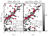 |
Fig. 10. Best-fit photometric vs. spectroscopic redshift for RUBIES sources with robust zspec > 3.1 (gray histogram) and the LRD sample (red hexagons; triangle indicates out of plot). Photometric redshifts were measured using eazy Brammer et al. 2008 with two different template sets: the blue_sfhz_13 set optimized for high-redshift galaxies (left) and the agn_blue_sfhz_13 set which includes an AGN template constructed from the LRD of Killi et al. 2024 and a torus model (right). The dashed lines show |Δz|/(1 + zspec) = 0.1. Although including this AGN template reduces the number of outliers and photometric redshift scatter for the LRD sample, a small bias toward higher photometric redshifts remains. |
Indeed, we find that the photometric redshift outliers are preferentially excluded by the photometric selections. Of the fourteen photometric redshift outliers in the magnitude-limited LRD sample, Barro et al. 2024 recovers seven (50%), Kocevski et al. 2025 recovers six (41%), while Kokorev et al. 2024 recovers only one (14%). Notably, all spectroscopic LRDs missed by two or more selection methods are redshift outliers. Among these are sources with very strong Balmer breaks, such as RUBIES-UDS-154183 (The Cliff; de Graaff et al. 2025b) and RUBIES-UDS-144195, the latter having such a strong Balmer break that it is instead fit as a Lyman break at zphot ∼ 14 (red triangle in Figure 10). Many of these strong break objects also demonstrate a turnover in the rest-optical and blue slopes at the reddest wavelengths. While our v-shape criteria selects them nonetheless, they may still miss more atypical or extreme cases. Although we find no such examples in our current sample, this remains a limitation of our color-based approach and may motivate broader selection strategies in future work.
Improving the completeness of future photometric selections will therefore require better treatment of the unusual colors of LRDs, which are currently not captured by commonly used template sets for photometric redshift fitting or not fully accounted for in the definition of color criteria. Recently, a dedicated LRD template was introduced in eazy, which was constructed from the LRD spectrum of Killi et al. 2024 combined with a hot dusty torus model that rises sharply in the near- to mid-infrared. We also test the inclusion of this template (agn_blue_sfhz_13) in the right panel Figure 10, and find that it sightly improves outlier fraction (fout = 0.39), scatter (σNMAD = 0.097), and median deviation (Δmed = 0.036)3. However, we note that a typical torus model may fail to properly describe LRDs as many have shown to have flat mid-IR colors not well described by hot dust Williams et al. 2024; Setton et al. 2025; Wang et al. 2025; de Graaff et al. 2025b; Chen et al. 2025a.
The success of photometric LRD selection hinges on accurately capturing their unique spectral properties. Although current methods achieve high accuracy in identifying LRDs, their incompleteness underscores the limitations of relying solely on broadband photometry. The high photometric redshift outlier fraction of spectroscopic LRDs, particularly among LRDs missed by both v-shaped and multi-color selection methods, suggests that standard high-redshift galaxy or AGN templates fail to fully describe LRD SEDs. In the future, developing new empirical LRD templates and combining complementary selection criteria may maximize photometric LRD completeness. Large spectroscopic campaigns like RUBIES will be essential to validate such photometric selections across the full color-morphology parameter space. Crucially, the simplicity of the RUBIES selection function, based primarily on a color–magnitude criterion without morphological pre-selection, enables the computation of completeness corrections across galaxy colors. While RUBIES is complete for the reddest sources, the survey also prioritizes the brightest sources and selects a large number of blue sources due to their relative abundance, ensuring that this study still recovers broad-line and LRD systems across the full color space.
6. Summary
We used the large spectroscopic dataset of JWST program RUBIES to quantify the characteristics commonly associated with LRDs – broad Balmer emission, v-shaped continua, point-like rest-optical morphologies – among the high-redshift galaxy population. Because the RUBIES targets span a wide range in color and redshift without any morphological pre-selection, they are uniquely positioned to determine the prevalence of each LRD characteristic across the galaxy population.
We presented one of the largest spectroscopic samples of broad Balmer line sources at high redshift to date, including 80 robust detections at z > 3.1, of which 28 (35%) lie at z > 6. Our detections are enabled by the unite package, which combines multiple NIRSpec spectra, i.e., the PRISM and G395M spectra, simultaneously to model emission lines and continua. This approach leverages the signal-to-noise ratio of the PRISM and the resolution of G395M to identify kinematic components of emission lines, overcoming limitations of single-disperser analyses.
Moreover, we used the RUBIES spectra to measure v-shaped continua, and measure detailed morphologies from NIRCam imaging to determine which sources are point-source dominated in the rest-optical. Remarkably, the definition of an LRD emerges naturally from the measured spectroscopic and photometric features: all point sources with (spectroscopic) v-shaped continua exhibit broad Balmer lines where the data quality permits detection. This strongly suggests that these three features are not coincidental, but likely stem from a common physical origin. This can possibly be explained in the context of the recently proposed phenomenon of a massive accreting black hole embedded in an envelope of dense gas Inayoshi & Maiolino 2025; Ji et al. 2025; Naidu et al. 2025; de Graaff et al. 2025b; Kido et al. 2025; Taylor et al. 2025b.
In detail, our primary findings can be summarized as follows:
-
The sample of broad Balmer line sources span a wide range in rest-optical broadband photometric colors, but are typically redder than the full RUBIES sample at z > 3.1 due to a combination of red rest-optical continua and high equivalent width emission lines.
-
The majority of sources with (spectroscopic) v-shaped continua also show a dominant point source component at rest-optical wavelengths. Remarkably, we robustly detect broad Balmer emission lines for upward of 80% of these sources; the remainder are inconclusive primarily due to data shortcomings. Similarly, the majority of sources with v-shaped continua show broad Balmer emission lines. Of this population, 80% also show a prominent point-source component in rest-optical imaging.
-
Strikingly, a population of sources with all three features emerges naturally from the data, and we therefore define this sample as spectroscopic LRDs, constituting the largest such sample (36) to date. Compared to the full sample of broad Balmer line sources, spectroscopic LRDs are the most luminous Hα emitters at any MUV.
-
Photometric LRD selections are highly accurate in their recovery of broad Balmer line sources (65−80%), as well as spectroscopic LRDs (up to ∼95% for F444W < 26.5). However, only 50−80% of the RUBIES LRDs were previously identified in these photometric searches, with higher completeness coming at the cost of LRD accuracy. In particular, the selections are increasingly incomplete for bluer broadband rest-optical colors and fainter UV magnitudes.
-
Combining multiple photometric LRD selections improves completeness but still leaves a large fraction of LRDs unrecovered. Sources that were missed typically have highly uncertain photometric redshifts and/or very strong Balmer breaks. This highlights the need for more nuanced photometric selection criteria as well as large spectroscopic surveys such as RUBIES.
With a clear definition of the spectro-photometric properties that select LRDs, we are now able to build a large robust sample of LRDs within RUBIES and the broader JWST spectroscopic archive. We can then begin to examine their detailed properties, such as the prevalence of Balmer absorption features and Balmer breaks, across the entire LRD population. In turn, this will provide critical clues about the evolutionary stages or environmental conditions of these systems, enabling a clearer understanding of their role in galaxy evolution and black hole growth.
Data availability
Full Table B.1 is available at the CDS via https://cdsarc.cds.unistra.fr/viz-bin/cat/J/A+A/702/A57
unite is hosted on GitHub with a v1 release coming soon.
We caution that the opposite is true for the general population of RUBIES sources, as Δ = −0.003, σNMAD = 0.037 and fout = 0.18 are all slightly worse than for the fits without an LRD template.
Acknowledgments
We would like to thank the anonymous reviewer for their constructive comments which improved the final manuscript. REH acknowledges support by the German Aerospace Center (DLR) and the Federal Ministry for Economic Affairs and Energy (BMWi) through program 50OR2403 ‘RUBIES’. TBM was supported by a CIERA Postdoctoral Fellowship. This work used computing resources provided by Northwestern University and the Center for Interdisciplinary Exploration and Research in Astrophysics (CIERA). This research was supported in part through the computational resources and staff contributions provided for the Quest high performance computing facility at Northwestern University which is jointly supported by the Office of the Provost, the Office for Research, and Northwestern University Information Technology. Support for this work was provided by The Brinson Foundation through a Brinson Prize Fellowship grant. The Cosmic Dawn Center is funded by the Danish National Research Foundation (DNRF) under grant #140. This work has received funding from the Swiss State Secretariat for Education, Research and Innovation (SERI) under contract number MB22.00072, as well as from the Swiss National Science Foundation (SNSF) through project grant 200020_207349. Support for this work for RPN was provided by NASA through the NASA Hubble Fellowship grant HST-HF2-51515.001-A awarded by the Space Telescope Science Institute, which is operated by the Association of Universities for Research in Astronomy, Incorporated, under NASA contract NAS5-26555. The work of CCW is supported by NOIRLab, which is managed by the Association of Universities for Research in Astronomy (AURA) under a cooperative agreement with the National Science Foundation. The data products presented herein were retrieved from the Dawn JWST Archive (DJA). DJA is an initiative of the Cosmic Dawn Center (DAWN). This work is based in part on observations made with the NASA/ESA/CSA James Webb Space Telescope. The data were obtained from the Mikulski Archive for Space Telescopes at the Space Telescope Science Institute, which is operated by the Association of Universities for Research in Astronomy, Inc., under NASA contract NAS 5-03127 for JWST. These observations are associated with programs numbers 1345, 1837, 2234, 2279, 2514, 2750, 3990 and 4233. Support for program no. 4233 was provided by NASA through a grant from the Space Telescope Science Institute, which is operated by the Association of Universities for Research in Astronomy, Inc., under NASA contract NAS 5-03127. The authors acknowledge the CEERS, PRIMER, PANORAMIC, and BEACONS teams for developing their observing program with a zero-exclusive-access period. We acknowledge the use of the following software packages which were instrumental in the development of this work: Astropy Astropy Collaboration 2013, 2018, 2022, grizli Brammer 2023a, jax Bradbury et al. 2018, jwst Bushouse et al. 2022, LaTeX Lamport 1994, MatplotlibHunter 2007, msaexp Brammer 2023b, msafit de Graaff et al. 2024, NumPy Oliphant 2006; van der Walt et al. 2011; Harris et al. 2020, NumPyro Phan et al. 2019, photutils Bradley et al. 2024b, pysersic Pasha & Miller 2023, photutils Bradley et al. 2024a, sedpy Johnson 2021, Source-Extractor Bertin & Arnouts 1996, and unite Hviding 2025. This work makes use of color palettes created by Martin Krzywinski designed for colorblindness. The color palettes and more information can be found at http://mkweb.bcgsc.ca/colorblind/
References
- Akins, H. B., Casey, C. M., Allen, N., et al. 2023, ApJ, 956, 61 [NASA ADS] [CrossRef] [Google Scholar]
- Akins, H. B., Casey, C. M., Lambrides, E., et al. 2024, ApJ, submitted [arXiv:2406.10341] [Google Scholar]
- Astropy Collaboration (Robitaille, T. P., et al.) 2013, A&A, 558, A33 [NASA ADS] [CrossRef] [EDP Sciences] [Google Scholar]
- Astropy Collaboration (Price-Whelan, A. M., et al.) 2018, AJ, 156, 123 [Google Scholar]
- Astropy Collaboration (Price-Whelan, A. M., et al.) 2022, ApJ, 935, 167 [NASA ADS] [CrossRef] [Google Scholar]
- Baggen, J. F. W., van Dokkum, P., Labbé, I., et al. 2023, ApJ, 955, L12 [NASA ADS] [CrossRef] [Google Scholar]
- Baggen, J. F. W., van Dokkum, P., Brammer, G., et al. 2024, ApJ, 977, L13 [NASA ADS] [CrossRef] [Google Scholar]
- Bagley, M. B., Finkelstein, S. L., Koekemoer, A. M., et al. 2023, ApJ, 946, L12 [NASA ADS] [CrossRef] [Google Scholar]
- Barro, G., Pérez-González, P. G., Kocevski, D. D., et al. 2024, ApJ, 963, 128 [CrossRef] [Google Scholar]
- Bertin, E., & Arnouts, S. 1996, A&AS, 117, 393 [NASA ADS] [CrossRef] [EDP Sciences] [Google Scholar]
- Bezanson, R., Labbe, I., Whitaker, K. E., et al. 2024, ApJ, 974, 92 [NASA ADS] [CrossRef] [Google Scholar]
- Boylan-Kolchin, M. 2023, Nat. Astron., 7, 731 [NASA ADS] [CrossRef] [Google Scholar]
- Bradbury, J., Frostig, R., Hawkins, P., et al. 2018, JAX: Composable Transformations of Python+NumPy Programs [Google Scholar]
- Bradley, L., Sipőcz, B., Robitaille, T., et al. 2024a, https://doi.org/10.5281/zenodo.12585239 [Google Scholar]
- Bradley, L., Sipőcz, B., Robitaille, T., et al. 2024b, https://doi.org/10.5281/zenodo.13989456 [Google Scholar]
- Brammer, G. 2023a, https://doi.org/10.5281/zenodo.1146904 [Google Scholar]
- Brammer, G. 2023b, https://doi.org/10.5281/zenodo.8319596 [Google Scholar]
- Brammer, G. B., van Dokkum, P. G., & Coppi, P. 2008, ApJ, 686, 1503 [Google Scholar]
- Brammer, G. B., van Dokkum, P. G., Franx, M., et al. 2012, ApJS, 200, 13 [Google Scholar]
- Burgasser, A. J., Bezanson, R., Labbe, I., et al. 2024, ApJ, 962, 177 [NASA ADS] [CrossRef] [Google Scholar]
- Bushouse, H., Eisenhamer, J., Dencheva, N., et al. 2022, https://doi.org/10.5281/zenodo.7229890 [Google Scholar]
- Carnall, A. C., Cullen, F., McLure, R. J., et al. 2024, MNRAS, 534, 325 [NASA ADS] [CrossRef] [Google Scholar]
- Casey, C. M., Kartaltepe, J. S., Drakos, N. E., et al. 2023, ApJ, 954, 31 [NASA ADS] [CrossRef] [Google Scholar]
- Chen, K., Li, Z., Inayoshi, K., Ho, L. C., et al. 2025a, ArXiv e-prints [arXiv:2505.22600] [Google Scholar]
- Chen, C.-H., Ho, L. C., Li, R., & Zhuang, M.-Y. 2025b, ApJ, 983, 60 [Google Scholar]
- Cooper, O. R., Brammer, G., Heintz, K. E., et al. 2025, ApJ, 982, 125 [Google Scholar]
- de Graaff, A., Rix, H.-W., Carniani, S., et al. 2024, A&A, 684, A87 [NASA ADS] [CrossRef] [EDP Sciences] [Google Scholar]
- de Graaff, A., Brammer, G., Weibel, A., et al. 2025a, A&A, 697, A189 [NASA ADS] [CrossRef] [EDP Sciences] [Google Scholar]
- de Graaff, A., Rix, H. W., Naidu, R. P., et al. 2025b, A&A, 701, A168 [NASA ADS] [CrossRef] [EDP Sciences] [Google Scholar]
- Donnan, C. T., McLure, R. J., Dunlop, J. S., et al. 2024, MNRAS, 533, 3222 [NASA ADS] [CrossRef] [Google Scholar]
- Finkelstein, S. L., Bagley, M. B., Arrabal Haro, P., et al. 2025, ApJ, 983, L4 [Google Scholar]
- Förster Schreiber, N. M., Übler, H., Davies, R. L., et al. 2019, ApJ, 875, 21 [Google Scholar]
- Furtak, L. J., Zitrin, A., Plat, A., et al. 2023, ApJ, 952, 142 [NASA ADS] [CrossRef] [Google Scholar]
- Furtak, L. J., Labbé, I., Zitrin, A., et al. 2024, Nature, 628, 57 [NASA ADS] [CrossRef] [Google Scholar]
- Galavis, M. E., Mendoza, C., & Zeippen, C. J. 1997, A&AS, 123, 159 [NASA ADS] [CrossRef] [EDP Sciences] [Google Scholar]
- Gardner, J. P., Mather, J. C., Abbott, R., et al. 2023, PASP, 135, 068001 [NASA ADS] [CrossRef] [Google Scholar]
- Gibson, J. L., Nelson, E., Williams, C. C., et al. 2024, ApJ, 974, 48 [Google Scholar]
- Greene, J. E., Labbe, I., Goulding, A. D., et al. 2024, ApJ, 964, 39 [CrossRef] [Google Scholar]
- Grogin, N. A., Kocevski, D. D., Faber, S. M., et al. 2011, ApJS, 197, 35 [NASA ADS] [CrossRef] [Google Scholar]
- Grudić, M. Y., Hopkins, P. F., Quataert, E., & Murray, N. 2019, MNRAS, 483, 5548 [CrossRef] [Google Scholar]
- Guia, C. A., Pacucci, F., & Kocevski, D. D. 2024, RNAAS, 8, 207 [Google Scholar]
- Habouzit, M. 2025, MNRAS, 537, 2323 [Google Scholar]
- Hainline, K. N., Helton, J. M., Johnson, B. D., et al. 2024, ApJ, 964, 66 [NASA ADS] [CrossRef] [Google Scholar]
- Hainline, K. N., Maiolino, R., Juodžbalis, I., et al. 2025, ApJ, 979, 138 [Google Scholar]
- Hao, L., Strauss, M. A., Fan, X., et al. 2005, AJ, 129, 1795 [NASA ADS] [CrossRef] [Google Scholar]
- Harikane, Y., Zhang, Y., Nakajima, K., et al. 2023, ApJ, 959, 39 [NASA ADS] [CrossRef] [Google Scholar]
- Harris, C. R., Millman, K. J., van der Walt, S. J., et al. 2020, Nature, 585, 357 [NASA ADS] [CrossRef] [Google Scholar]
- Heintz, K. E., Brammer, G. B., Watson, D., et al. 2025, A&A, 693, A60 [Google Scholar]
- Hoffman, M. D., & Gelman, A. 2014, J. Mach. Learn. Res., 15, 1593 [Google Scholar]
- Hopkins, P. F., Murray, N., Quataert, E., & Thompson, T. A. 2010, MNRAS, 401, L19 [NASA ADS] [Google Scholar]
- Hunter, J. D. 2007, Comput. Sci. Eng., 9, 90 [NASA ADS] [CrossRef] [Google Scholar]
- Hviding, R. E. 2025, https://doi.org/10.5281/zenodo.15585035 [Google Scholar]
- Hviding, R., de Graaff, A., Setton, D., Miller, T., & Greene, J. 2025, https://doi.org/10.5281/zenodo.15528783 [Google Scholar]
- Inayoshi, K., & Maiolino, R. 2025, ApJ, 980, L27 [Google Scholar]
- Ji, X., Maiolino, R., Übler, H., et al. 2025, MNRAS, submitted [arXiv:2501.13082] [Google Scholar]
- Johnson, B. D. 2021, https://doi.org/10.5281/zenodo.4582723 [Google Scholar]
- Juodžbalis, I., Maiolino, R., Baker, W. M., et al. 2025, MNRAS, submitted [arXiv:2504.03551] [Google Scholar]
- Kido, D., Ioka, K., Hotokezaka, K., Inayoshi, K., & Irwin, C. M. 2025, MNRAS, submitted [arXiv:2505.06965] [Google Scholar]
- Killi, M., Watson, D., Brammer, G., et al. 2024, A&A, 691, A52 [NASA ADS] [CrossRef] [EDP Sciences] [Google Scholar]
- Kocevski, D. D., Onoue, M., Inayoshi, K., et al. 2023, ApJ, 954, L4 [NASA ADS] [CrossRef] [Google Scholar]
- Kocevski, D. D., Finkelstein, S. L., Barro, G., et al. 2025, ApJ, 986, 126 [Google Scholar]
- Koekemoer, A. M., Faber, S. M., Ferguson, H. C., et al. 2011, ApJS, 197, 36 [NASA ADS] [CrossRef] [Google Scholar]
- Kokorev, V., Fujimoto, S., Labbe, I., et al. 2023, ApJ, 957, L7 [NASA ADS] [CrossRef] [Google Scholar]
- Kokorev, V., Caputi, K. I., Greene, J. E., et al. 2024, ApJ, 968, 38 [NASA ADS] [CrossRef] [Google Scholar]
- Labbé, I., van Dokkum, P., Nelson, E., et al. 2023, Nature, 616, 266 [CrossRef] [Google Scholar]
- Labbe, I., Greene, J. E., Matthee, J., et al. 2024, ApJ, submitted [arXiv:2412.04557] [Google Scholar]
- Labbe, I., Greene, J. E., Bezanson, R., et al. 2025, ApJ, 978, 92 [NASA ADS] [CrossRef] [Google Scholar]
- Lamport, L. 1994, LaTeX: A Document Preparation System, 2nd edn. (Addison-Wesley Professional) [Google Scholar]
- Langeroodi, D., & Hjorth, J. 2023, ApJ, 957, L27 [NASA ADS] [CrossRef] [Google Scholar]
- Larson, R. L., Finkelstein, S. L., Kocevski, D. D., et al. 2023, ApJ, 953, L29 [NASA ADS] [CrossRef] [Google Scholar]
- Leung, G. C. K., Coil, A. L., Aird, J., et al. 2019, ApJ, 886, 11 [NASA ADS] [CrossRef] [Google Scholar]
- Li, J., Silverman, J. D., Shen, Y., et al. 2025, ApJ, 981, 19 [Google Scholar]
- Lin, X., Wang, F., Fan, X., et al. 2024, ApJ, 974, 147 [NASA ADS] [CrossRef] [Google Scholar]
- Lin, X., Fan, X., Wang, F., et al. 2025, ApJ, submitted [arXiv:2504.08039] [Google Scholar]
- Ma, Y., Greene, J. E., Setton, D. J., et al. 2025, ApJ, 981, 191 [Google Scholar]
- Maiolino, R., Scholtz, J., Curtis-Lake, E., et al. 2024, A&A, 691, A145 [NASA ADS] [CrossRef] [EDP Sciences] [Google Scholar]
- Matthee, J., Naidu, R. P., Brammer, G., et al. 2024, ApJ, 963, 129 [NASA ADS] [CrossRef] [Google Scholar]
- Naidu, R. P., Matthee, J., Kramarenko, I., et al. 2024, Open J. Astrophys., submitted [arXiv:2410.01874] [Google Scholar]
- Naidu, R. P., Matthee, J., Katz, H., et al. 2025, Nature, submitted [arXiv:2503.16596] [Google Scholar]
- Oke, J. B., & Gunn, J. E. 1983, ApJ, 266, 713 [NASA ADS] [CrossRef] [Google Scholar]
- Oliphant, T. E. 2006, A Guide to NumPy (USA: Trelgol Publishing), 1 [Google Scholar]
- Pasha, I., & Miller, T. B. 2023, JOSS, 8, 5703 [Google Scholar]
- Pérez-González, P. G., Barro, G., Annunziatella, M., et al. 2023, ApJ, 946, L16 [CrossRef] [Google Scholar]
- Pérez-González, P. G., Barro, G., Rieke, G. H., et al. 2024, ApJ, 968, 4 [CrossRef] [Google Scholar]
- Phan, D., Pradhan, N., & Jankowiak, M. 2019, ArXiv e-prints [arXiv:1912.11554] [Google Scholar]
- Pizzati, E., Hennawi, J. F., Schaye, J., et al. 2025, MNRAS, 539, 2910 [Google Scholar]
- Rinaldi, P., Bonaventura, N., Rieke, G. H., et al. 2024, ApJ, submitted [arXiv:2411.14383] [Google Scholar]
- Rusakov, V., Watson, D., Nikopoulos, G. P., et al. 2025, Nature, submitted [arXiv:2503.16595] [Google Scholar]
- Setton, D. J., Greene, J. E., de Graaff, A., et al. 2024, ApJ, submitted [arXiv:2411.03424] [Google Scholar]
- Setton, D. J., Greene, J. E., Spilker, J. S., et al. 2025, ApJ, submitted [arXiv:2503.02059] [Google Scholar]
- Skelton, R. E., Whitaker, K. E., Momcheva, I. G., et al. 2014, ApJS, 214, 24 [Google Scholar]
- Sun, F., Fudamoto, Y., Lin, X., et al. 2025, ApJS, submitted [arXiv:2503.15587] [Google Scholar]
- Taylor, A. J., Finkelstein, S. L., Kocevski, D. D., et al. 2025a, ApJ, 986, 165 [Google Scholar]
- Taylor, A. J., Kokorev, V., Kocevski, D. D., et al. 2025b, ApJ, accepted [arXiv:2505.04609] [Google Scholar]
- Valentino, F., Brammer, G., Gould, K. M. L., et al. 2023, ApJ, 947, 20 [NASA ADS] [CrossRef] [Google Scholar]
- van der Walt, S., Colbert, S. C., & Varoquaux, G. 2011, Comput. Sci. Eng., 13, 22 [Google Scholar]
- Wang, B., Leja, J., de Graaff, A., et al. 2024, ApJ, 969, L13 [NASA ADS] [CrossRef] [Google Scholar]
- Wang, B., de Graaff, A., Davies, R. L., et al. 2025, ApJ, 984, 121 [Google Scholar]
- Watanabe, S., & Opper, M. 2010, J. Mach. Learn. Res., 11, 1243 [Google Scholar]
- Weibel, A., Oesch, P. A., Barrufet, L., et al. 2024, MNRAS, 533, 1808 [NASA ADS] [CrossRef] [Google Scholar]
- Weibel, A., de Graaff, A., Setton, D. J., et al. 2025, ApJ, 983, 11 [Google Scholar]
- Williams, C. C., Alberts, S., Ji, Z., et al. 2024, ApJ, 968, 34 [NASA ADS] [CrossRef] [Google Scholar]
- Williams, C. C., Oesch, P. A., Weibel, A., et al. 2025, ApJ, 979, 140 [Google Scholar]
- Xiao, M., Williams, C. C., Oesch, P. A., et al. 2025, A&A, 696, A156 [NASA ADS] [CrossRef] [EDP Sciences] [Google Scholar]
- Zhuang, M. Y., Li, J., Shen, Y., et al. 2025, ApJ, submitted [arXiv:2505.20393] [Google Scholar]
Appendix A: LRDs from RUBIES
We present all spectroscopically identified LRDs from RUBIES, along with all v-shaped and unresolved sources where we are unable to identify broad lines due to data quality limitations. We identify a total of 36 spectroscopic LRDs and seven additional sources with v-shaped continua and dominant rest-optical point sources. In Figure A.1 we present the color images (constructed from the F444W, F277W and F150W NIRCam filters), PRISM spectra, and G395M zoom-ins of the Hα broad emission for all 43 objects. Key properties of spectroscopic LRDs and unresolved v-shaped galaxies are provided in Tables A.1 and A.2 respectively. We caution that the reported broad Balmer FWHM values are derived from Gaussian fitting with FWHM < 2500 km s−1 that may not best represent the spectral profile. In Table A.2 we also include the reason why each unresolved v-shaped galaxy has an indeterminate broad line, i.e., due to a DQ issue or missing forbidden or Balmer line.
RUBIES spectroscopic LRDs
RUBIES v-shaped rest-optical point sources (with indeterminate broad Balmer emission)
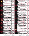 |
Fig. A.1. All RUBIES LRDs (red) found in this work followed by rest-optical point sources with v-shaped continua (orange) all organized by redshift. In each column in each row we show the following: the 1″ × 1″ F444W/F277W/F150W RGB cutouts (left), the log-scaled PRISM spectra with the location of the Balmer limit marked with a dashed line (middle), and the linear-scaled G395M ±3000 km s−1 zoom-in of the Hα line where available, otherwise Hβ, with the broad unite fit superimposed (right). |
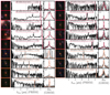 |
Fig. A.2. All RUBIES LRDs (red) found in this work followed by rest-optical point sources with v-shaped continua (orange) all organized by redshift. In each column in each row we show the following: the 1″ × 1″ F444W/F277W/F150W RGB cutouts (left), the log-scaled PRISM spectra with the location of the Balmer limit marked with a dashed line (middle), and the linear-scaled G395M ±3000 km s−1 zoom-in of the Hα line where available, otherwise Hβ, with the broad unite fit superimposed (right) (continued). |
Appendix B: Broad line sample
We present the results of our broad-line fitting, including both successful detections and cases where our fitting procedure failed due to data quality issues. In Figure B.1 we show how trace overlaps in G395M or other data quality artifacts can produce a bad fit with a broad line:
-
RUBIES-UDS-42150: Here the Hα emission falls at the edge of the G395M spectral range, leading to data quality issues.
-
RUBIES-UDS-822719: Emission line contamination from an adjacent trace can artificially induce flux in the G395M that can be better fit with a broad component.
-
RUBIES-EGS-67278: Trace overlap may also manifest as additional continuum flux in the G395M spectrum, leading to a bad fit with a broad line.
-
RUBIES-EGS-11752: In rare cases, a line might be missing entirely from the G395M data
Our analysis identified 80 robust broad Balmer line sources and 18 potential broad-line systems The complete catalog of broad-line sources is provided in Table B.1, while Figure B.2 shows spectral zoom-ins for all robust and potential broad-line systems. However, we caution that the reported broad Balmer FWHM values are derived from Gaussian fitting with FWHM < 2500 km s−1, optimized for broad line detection, that may not best represent the spectral profile.
RUBIES zspec > 3.1 broad Balmer line galaxies
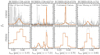 |
Fig. B.1. Examples of failed fits due to artifacts at the edge of the spectral range, emission line contamination from trace overlaps, continuum contamination from trace overlaps, and inconsistencies between G395M and PRISM extractions for RUBIES-UDS-42150, RUBIES-UDS-822719, RUBIES-EGS-67278, and RUBIES-EGS-11752 respectively. |
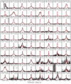 |
Fig. B.2. All robust broad Balmer line objects found in the RUBIES data, organized by redshift. We plot the linear-scaled G395M ±3000 km s−1 zoom-in of the Hα line where available, otherwise Hβ, with the broad unite fit superimposed in red and the broad Balmer component in orange. We also include text containing the FWHM of the broad component. |
All Tables
RUBIES v-shaped rest-optical point sources (with indeterminate broad Balmer emission)
All Figures
|
Fig. 1. Diversity of red high-redshift sources in RUBIES. Right: F115W−F200W vs. F277W−F444W for RUBIES sources with robust zspec > 3.1 (gray histogram), which populate a broad distribution in color space. Right: PRISM spectra and NIRCam photometry, G395M spectra (zoomed in on Hα), and 1″ × 1″ NIRCam F444W/F277W/F150W RGB images for three RUBIES targets that are close in color space. The top row shows a typical LRD, with a v-shaped continuum, broad Hα emission line and very compact morphology. The middle row shows an extended red object with a v-shaped continuum, but narrow Hα and [N II] emission. The red source in the bottom row is a point source with a relatively blue continuum, but appears as red due to high equivalent width emission lines, including a broad Hα line. This demonstrates that sources with similar broadband photometric colors can have very different spectral properties. |
| In the text | |
|
Fig. 2. Zoomed-in images of the spectroscopic fits for RUBIES-EGS-926125 (left) and RUBIES-EGS-966323 (right) using narrow (blue) and broad (orange) models for both G395M (top) and PRISM (bottom) spectra along with their residual deviations. We plot the maximum posterior sample from the MCMC fitting. Simultaneous fitting leverages all available data to constrain linewidths in both gratings across different wavelength regimes. For 926125 we show both the Hβ + [O III] and Hα + [N II] complexes, while for 966323 we only have coverage of the Hβ + [O III] complex. We note that a broad component could not be conclusively fit in 966323 from the PRISM or G395M spectrum alone in Wang et al. 2024 or Kocevski et al. 2025, but is detected in this work at the > 6.5σ level. |
| In the text | |
|
Fig. 3. Rest-UV (blue) and rest-optical (orange) continuum fitting of RUBIES-EGS-42046 (top) and RUBIES-UDS-934230 (bottom) from PRISM spectroscopy (solid) and NIRCam photometry (dashed). In the insets are the 0.5″ × 0.5″ NIRCam F444W/F277W/F150W RGB cutouts of the sources. We emphasize that spectroscopic rest-optical continuum fitting can mitigate the effect of strong emission lines, but can suffer in S/N in the rest-UV where the spectrum is fainter or cannot capture extended rest-UV emission due to slit losses. RUBIES-EGS-42046 is identified as a spectroscopic v-shape, while RUBIES-UDS-934230 is not despite a red photometric rest-optical color. |
| In the text | |
|
Fig. 4. Stellar locus and morphological classification in LW NIRCam filters. The black stars show the 95th percentile effective radius posterior (reff, 95%) vs. magnitude for reference stars, with the best-fit stellar locus (gray dashed line). We classify galaxies as point sources (green hashed area) if they fall below the +4σresid offset of this relation (rrsv; green line). The gray circles show all RUBIES sources with robust zspec > 3.1, red hexagons highlight spectroscopic LRDs (Section 4.2), and black circles mark non-LRD sources with dominant point-sources (Section 3.3.1), plotted in the LW filter that traces the rest-5500 Å flux. |
| In the text | |
|
Fig. 5. Color-color space distribution of RUBIES sources with robust zspec > 3.1 (gray histogram). We divide the sample into zspec < 5 (right) and zspec > 5 (left) and show the NIRCam F090W−F150W vs. F200W−F356W and F115W−F200W vs. F277W−F444W, respectively, which approximately probe rest-UV vs. rest-optical colors. In the top row we plot objects that satisfy our condition for broad-line, unresolved, and v-shaped features, along with their combinations, above the full distributions of the parent sample in each redshift regime. In the bottom row we plot the objects that satisfy all three criteria. Each panel includes the total number of objects shown and the fraction of the represented sample. The points are colored as in Figure 7. |
| In the text | |
|
Fig. 6. βUV − βopt space distribution of RUBIES sources with robust zspec > 3.1 (gray histogram). On the right, we plot objects that satisfy our condition for broad-line, unresolved, and v-shaped features, along with their combinations, above the full distributions of the parent sample. On the left, we plot the objects that satisfy all three criteria. The slopes are derived from PRISM spectroscopy and each panel includes the total number of objects plotted and their fraction of the represented sample. The points are colored as in Figure 7. |
| In the text | |
|
Fig. 7. Left: Euler diagram displaying the overlap between the three LRD characteristic criteria: a broad Balmer line, a dominant point source component at rest-optical wavelengths, and a spectroscopic v-shaped continuum. Right: Histogram showing the composition of overlaps in the Euler diagram where only two of the three features are measured. We note that objects with a rest-optical point source and a v-shaped continuum are 80% likely to have a broad line. In fact, in the remaining 20% we cannot reject a broad line, but our quality cuts restrict us from being fully confident. This suggests an underpinning physical link between the three LRD features. |
| In the text | |
|
Fig. 8. Left: Redshift vs. NIRCam F356W (for zspec ≤ 5) or F444W (for zspec > 5). Right: Absolute UV magnitude (MUV) at 1500 Å, derived from rest-UV spectroscopic slopes, is plotted against total, narrow plus broad, Hα luminosity. RUBIES sources with robust zspec > 3.1 are shown as a gray histogram. Broad-line sources are indicated with dark red circles, and LRDs, defined as galaxies with v-shaped continua, broad Balmer lines, and dominant rest-optical point sources, are shown as light red hexagons. At fixed LHα, LRDs are faint in the rest-UV compared to the full population. Conversely, extreme Hα emitters (LHα ≳ 1010 M⊙) are dominated by LRDs, i.e., LRDs constitute the most luminous Hα emitters at fixed UV luminosity. |
| In the text | |
|
Fig. 9. Breakdown of photometric LRD selection methods at F444W < 26.5. The left panel shows how photometric LRDs are distributed among spectroscopically classified categories: spectroscopic LRDs (red), rest-optical point sources and v-shaped galaxies (orange), broad Balmer line sources (dark red), non-LRDs (black), and galaxies with unreliable feature measurements (gray hatched). Overall, photometric LRD selections are accurate but incomplete relative to spectroscopic identifications. The right panel investigates the completeness of the RUBIES photometric LRDs as a function of F277W−F444W color (left) and F115W magnitude (right). The top plots show histograms of RUBIES LRDs (red), matched LRDs from Kocevski et al. (2025, orange), and Kokorev et al. (2024, blue). The bottom plots display the binned completeness of each selection method relative to the RUBIES sample. We find that Kocevski et al. 2025 is incomplete at bluer colors, while Kokorev et al. 2024 is primarily incomplete at fainter rest-UV magnitudes. |
| In the text | |
|
Fig. 10. Best-fit photometric vs. spectroscopic redshift for RUBIES sources with robust zspec > 3.1 (gray histogram) and the LRD sample (red hexagons; triangle indicates out of plot). Photometric redshifts were measured using eazy Brammer et al. 2008 with two different template sets: the blue_sfhz_13 set optimized for high-redshift galaxies (left) and the agn_blue_sfhz_13 set which includes an AGN template constructed from the LRD of Killi et al. 2024 and a torus model (right). The dashed lines show |Δz|/(1 + zspec) = 0.1. Although including this AGN template reduces the number of outliers and photometric redshift scatter for the LRD sample, a small bias toward higher photometric redshifts remains. |
| In the text | |
|
Fig. A.1. All RUBIES LRDs (red) found in this work followed by rest-optical point sources with v-shaped continua (orange) all organized by redshift. In each column in each row we show the following: the 1″ × 1″ F444W/F277W/F150W RGB cutouts (left), the log-scaled PRISM spectra with the location of the Balmer limit marked with a dashed line (middle), and the linear-scaled G395M ±3000 km s−1 zoom-in of the Hα line where available, otherwise Hβ, with the broad unite fit superimposed (right). |
| In the text | |
|
Fig. A.2. All RUBIES LRDs (red) found in this work followed by rest-optical point sources with v-shaped continua (orange) all organized by redshift. In each column in each row we show the following: the 1″ × 1″ F444W/F277W/F150W RGB cutouts (left), the log-scaled PRISM spectra with the location of the Balmer limit marked with a dashed line (middle), and the linear-scaled G395M ±3000 km s−1 zoom-in of the Hα line where available, otherwise Hβ, with the broad unite fit superimposed (right) (continued). |
| In the text | |
|
Fig. B.1. Examples of failed fits due to artifacts at the edge of the spectral range, emission line contamination from trace overlaps, continuum contamination from trace overlaps, and inconsistencies between G395M and PRISM extractions for RUBIES-UDS-42150, RUBIES-UDS-822719, RUBIES-EGS-67278, and RUBIES-EGS-11752 respectively. |
| In the text | |
|
Fig. B.2. All robust broad Balmer line objects found in the RUBIES data, organized by redshift. We plot the linear-scaled G395M ±3000 km s−1 zoom-in of the Hα line where available, otherwise Hβ, with the broad unite fit superimposed in red and the broad Balmer component in orange. We also include text containing the FWHM of the broad component. |
| In the text | |
Current usage metrics show cumulative count of Article Views (full-text article views including HTML views, PDF and ePub downloads, according to the available data) and Abstracts Views on Vision4Press platform.
Data correspond to usage on the plateform after 2015. The current usage metrics is available 48-96 hours after online publication and is updated daily on week days.
Initial download of the metrics may take a while.