| Issue |
A&A
Volume 702, October 2025
|
|
|---|---|---|
| Article Number | A231 | |
| Number of page(s) | 11 | |
| Section | The Sun and the Heliosphere | |
| DOI | https://doi.org/10.1051/0004-6361/202556009 | |
| Published online | 22 October 2025 | |
Formation of Si IV due to the interaction of an electron beam with the flaring solar chromosphere
Astronomical Institute of the Czech Academy of Sciences, Fričova 298, Ondřejov, Czech Republic
⋆ Corresponding author: This email address is being protected from spambots. You need JavaScript enabled to view it.
Received:
18
June
2025
Accepted:
26
August
2025
Abstract
Aims. We modeled Si IV emission at the footpoints of flaring loops to evaluate the effects of the electron beam, non-equilibrium ionization, and suppression of dielectronic recombination.
Methods. The radiation-hydrodynamic code FLARIX was used to model the properties of plasma in solar flare ribbons. Energy was deposited via short-duration electron beams with a triangular profile in time, peaking at 1, 3, or 5 s, and with an energy flux ranging from 1 to 9 × 1010 cm−2 s−1. Subsequently, we calculated the non-equilibrium ionization states of silicon, taking into account the non-Maxwellian electron distribution containing the electron beam component. The Si IV line intensities and their evolution in time were modeled using a 161-level CHIANTI ion model.
Results. We found that the maximum of Si IV emissivity occurs in a “hot bubble” formed at the location of the maximum of beam energy deposition. The non-equilibrium abundances of Si IV were found to differ from those of the equilibrium by more than one order of magnitude. The ionization by the electron beam has only a small effect on the Si IV emissivity; typically below 10%. However, the effect of density suppression of dielectronic recombination is much more important, as the emissivities calculated without it can be several times lower than when this effect is included. Overall, the main contribution to the total intensity of Si IV lines along the flare loop comes from the hot bubble in optically thin cases or from plasma above this bubble when the plasma is optically thick.
Conclusions. Non-equilibrium ionization and density suppression of dielectronic recombination are found to be important effects influencing the modeled ionization states of the flaring plasma and the resulting Si IV emissivities. For short-duration electron beams, the maximum of the emissivity corresponds to the position of the hot bubble.
Key words: Sun: activity / Sun: chromosphere / Sun: flares / Sun: transition region / Sun: UV radiation
© The Authors 2025
 Open Access article, published by EDP Sciences, under the terms of the Creative Commons Attribution License (https://creativecommons.org/licenses/by/4.0), which permits unrestricted use, distribution, and reproduction in any medium, provided the original work is properly cited.
This article is published in open access under the Subscribe to Open model. This email address is being protected from spambots. You need JavaScript enabled to view it. to support open access publication.
1. Introduction
Solar flares are dynamic, energetic, and strongly radiating phenomena in the solar atmosphere. They release enormous amounts of magnetic energy, which is subsequently transported from the solar corona to the lower atmosphere. The energy is thought to be transported mainly by an accelerated electron beam (Brown 1971; Hoyng et al. 1976). The non-thermal electrons move along magnetic field lines through the transition region to the chromosphere, where they deposit their energy (e.g., Brown 1971; Emslie 1978; Holman et al. 2011).
The transition region is a thin interface region between the chromosphere and corona. The emission of transition region (TR) ions is currently observed with the Interface Region Imaging Spectrograph (IRIS). Its 1400 Å spectral window allows for observations of the Si IV doublet lines at 1393.75 Å and 1402.77 Å (see De Pontieu et al. 2014; Dudík et al. 2014a) as well as several other O IV and S IV lines. The transition region is long known to react quite fast to energy deposition during solar flares, leading to the increase in line intensities (see, e.g., Cheng et al. 1982; Tandberg-Hanssen et al. 1983; Hudson et al. 1994, or the cartoon summary in Benz 2008).In addition to fast increase in line intensities, significant line broadening as well as red shifts up to 100 km s−1 are often observed (e.g., Tian et al. 2015; Warren et al. 2016; Li et al. 2017). In rare instances, the lines can also be blueshifted (see Lörinčík et al. 2022a). The fast response of the transition region to energy deposition is of importance, since the observed HXR bursts are known to be of sub-second duration (e.g., Kiplinger et al. 1983; Aschwanden et al. 1995; Qiu et al. 2012; Cheng et al. 2012; Knuth & Glesener 2020) while the flaring chromosphere and transition region are also known to be heated by relatively short bursts (see also García-Rivas et al. 2024) or they exhibit variations on timescales of seconds (e.g., Jeffrey et al. 2018). In this respect, we note that the three-dimensional slipping or slip-running reconnection (e.g., Aulanier et al. 2006; Janvier et al. 2013; Dudík et al. 2014b, 2016; Sobotka et al. 2016; Li & Zhang 2014, 2015; Li et al. 2016; Lörinčík et al. 2019, 2022a, 2025), where the reconnecting field line footpoints exhibit motion along solar flare ribbons, necessarily indicates that a particular location within the flaring chromosphere has variable (and short-duration) energy deposition.
Furthermore, the ratio of line intensities of the Si IV doublet is, in optically thin conditions, constant, being close to 2 (e.g., Dudík et al. 2014a). However, the observations show that the ratio can often deviate from this value, presumably due to opacity effects and possibly outside flares as well (see, e.g., Yan et al. 2015; Tripathi et al. 2020; Zhou et al. 2022, 2024; Babu et al. 2024).
The formation of Si IV was modeled, for example, by Rubio da Costa et al. (2015). These authors used RADYN simulations and CHIANTI data to model the time evolution of Doppler shift of Si IV for duration of the beam energy deposition up to 120 s. They found significant Doppler shifts after 20 s of the energy deposition which increased with time. Kerr et al. (2019) simulated Si IV emission formed by electron beam under the assumption of non-LTE, non-equilibrium level populations, and with included radiation transfer for RADYN flaring atmospheres. They also tabulated physical parameters of the electron beam with opacity effects. Also, Reep et al. (2016, 2018) provided a comparison of multithreaded loop simulations versus single-loop simulations to reproduce the observed red line shifts. Nanoflare simulations driven by electron beam using HYDrodynamics and RADiation code (HYDRAD, Bradshaw & Mason 2003a) performed by Polito et al. (2018) showed that observed Doppler motions were consistent with the electron beam scenario for heating duration of 50–100 s and high energy fluxes.
This paper is organized as follows: Section 2 describes FLARIX model and input model parameters. Section 3 presents a calculation of the time-dependent Si ionization state, ionization and recombination rates, effect of the electron beam and density suppression of dielectronic recombination on the Si IV emissivity. Results of modeling are presented in Sect. 4 and a short summary is given in Sect. 5.
2. Model
The heating of low-lying solar atmospheric levels from the chromosphere to the transition region during solar flares is understood as a response to the energy transport by an electron beam from its injection in the reconnection region down to the chromosphere.
To model the response of the chromosphere and transition region to the energy release of the electron beam, we performed simulations using FLARIX code (Varady et al. 2010; Kašparová et al. 2019) developed at our Institute. It is a 1D non-LTE radiation hydrodynamic code similar to RADYN (Carlsson & Stein 1992, 1997; Abbett & Hawley 1999; Allred et al. 2005, 2015; Kerr 2022). RADYN and FLARIX differ mainly in the numerical schemes. For example, FLARIX uses a fixed grid optimized to capture atmosphere structure changes during the adopted heating, while RADYN uses an adaptive grid. Comparison of both models was performed by Kašparová et al. (2019), who found a close agreement between the time evolution of the modeled flaring atmosphere structure. Usually, the FLARIX code is used to model the chromospheric emission in optically thick lines such as Hα, Ca II, or Mg II (Kašparová et al. 2009; Radziszewski et al. 2024). So far, it has not been used to model the transition region lines.
Here, we used FLARIX to model time-dependent plasma parameters in the flaring atmosphere. Radiative transfer was treated in detail for atoms and ions important for radiative losses, such as H, Ca II, and Mg II. The non-equilibrium ionization of hydrogen was also taken into account. Optically thin radiative losses for other ions were calculated using the CHIANTI database (Dere et al. 1997; Del Zanna et al. 2021). The outputs of FLARIX are plasma parameters such as temperature, electron density, velocity, energy deposition, and so on, recorded with a time step of 0.1 s. The VAL C (Fig. 1 in Vernazza et al. 1981) atmosphere corresponding to a quiet Sun state was used as an initial atmosphere.
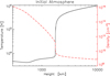 |
Fig. 1. Temperature (black line) and electron density (red dashed line) in the initial VAL C atmosphere. |
For the calculation of the Si IV non-equilibrium ionization state and Si IV emission, we assumed a Maxwell distribution for thermal electrons (with temperature corresponding to instantaneous temperature), together with a distribution of the electron beam corresponding to the given column depth at each height in the atmosphere. We assumed a power-law electron distribution of the electron beam with low-energy cutoff of 20, 15, and 10 keV and power-law indexes 3, 4, 5, and 6. The resulting electron distribution that includes this beam is thus non-Maxwellian. The maximum flux of the electron beam (1–9 × 10¹⁰ erg cm−2 s−1) was modulated by a triangular function (Fig. 2) with a maximum occurring either at 1 s, 3 s, or 5 s. Such short heating durations were chosen for two reasons. First, the set of F-CHROMA RADYN models (Carlsson et al. 2023) corresponds to 10 s and it is not necessary to repeat their calculations. Second, the energy release via the process of slipping reconnection (Aulanier et al. 2006, 2012; Janvier et al. 2013; Dudík et al. 2014b, 2016; Sobotka et al. 2016; Lörinčík et al. 2019, 2025) can be quite fast, with individual moving kernels or flare loops moving through a given location in the flare ribbon during only a short time. Consequently, the duration of energy deposition (beam interaction with the chromosphere) also needs to be quite short. Consequently, the time-dependent relative non-equilibrium abundances of Si IV, including the effect of the electron beam on the ionization rates, were calculated with temporal resolution 0.1 s, which is sufficient to capture the evolution of the Si IV intensities. The full 161-level CHIANTI model of Si IV was used to determine time-dependent Si IV emission. Finally, we selected six models to show the effect of changing of the beam parameters on Si IV abundance and line emission.
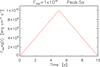 |
Fig. 2. Triangular flux modulation with the peak at 5 s. |
3. Formation of the Si IV line
To calculate the intensity of the IRIS Si IV line at 1402.8 Å, along with its evolution at each grid point of the model, we need to obtain both the relative fraction of the Si IV ion, as well as the relative population of its energy levels. Since there is rapid energy deposition in the model, the ionization fractions of the Si IV cannot be expected to be in ionization equilibrium at each instant in time. This is because even in collisionally dominated plasmas, the corresponding equilibration timescales for Si at transition region temperatures can be of the order of 3–10 s at typical transition region densities of log(Ne [cm−3]) = 11 (Smith & Hughes 2010). At lower densities, the equilibration timescales are correspondingly longer. Similarly, the equilibration timescales can be even longer if there are plasma flows through the transition region (e.g., Bradshaw & Mason 2003a,b; Olluri et al. 2013).
3.1. Si IV ionization fractions
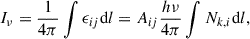
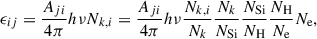
For the calculation of the Si IV fractions out of equilibrium, we assumed that the ionization is dominated by direct ionization and autoionization, while recombination occurs primarily via radiative and dielectronic recombination. The time-dependent changes of the abundance of ion Ni can be written as
 (1)
(1)
where Nk is the density of ions in the ionization state, k; Ik − 1 → k is the total ionization rate from state k − 1 to k; Rk + 1 → k is the total recombination rate, Ne is the electron density, r is the coordinate along the modeled loop, and v is the plasma velocity.
In all studied cases, the velocities, v, are relatively low in the region where Si IV has a significant abundance and the factor v dNk/dr is approximately at least one order lower than dNk/dt. Therefore, it could be omitted in our calculations.
3.1.1. Ionization rates
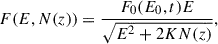
The distribution of electrons involved in collisions that lead to direct ionization or autoionization is assumed to be composed of two parts: (1) a Maxwellian corresponding to the temperature of the heated atmosphere and (2) a beam given by the beam energy distribution at a given height of the transition region at given time. We assumed that the initial power-law flux distribution of the electron beam F0(E0, t) [cm−2 s−1 erg−1 ] can be expressed as (Nagai & Emslie 1984):
 (2)
(2)
where δ is the power-law index, g(t) is a function of the flux time modulation (Fig. 2), Emin is the low energy cutoff, and Fmax [erg cm−2 s−1] is
 (3)
(3)
For the flux distribution in depth z with column depth N(z) we can write
 (4)
(4)
where
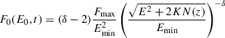 (5)
(5)
and K = 2πe4Λ (Brown 1972).
The ionization rate for the electron beam RebI can be written
 (6)
(6)
where σ is the cross-section for direct ionization or autoionization, me is electron mass, and f(v) is particle distribution of velocities.
Direct ionization and autoionization rates, RMaxw, for the Maxwellian distribution together with their cross-sections required for the calculation of the beam ionization were taken from the CHIANTI atomic database v. 10.0 (Del Zanna et al. 2021).
3.1.2. Recombinaton rates
Dielectronic recombination (DR) is an important contributor to total recombination. This process proceeds through the excited high levels. After a capture of a free electron, the recombining ion is temporarily in a doubly excited state. Subsequently, the ion can be stabilized through radiative decay. However, at relatively high electron densities, the probability of collisional ionization of the doubly excited ion, before it can decay radiatively, is increased. This reionization effectively suppresses the dielectronic recombination rates (e.g., Burgess & Summers 1969; Nikolić et al. 2013).
The published DR rates are usually calculated only in the limit of electron density being close to zero; that is, no suppression is present. However, already Burgess & Summers (1969) showed that the density suppression of dielectronic recombination is important even for low coronal densities of log(Ne [cm−3]) = 8. In the transition region, and even at higher densities in the flaring atmosphere, this effect is much more significant. Recently, Nikolić et al. (2013, 2018) developed a general model to calculate the density-dependent DR rate for Maxwellian distribution. Following them, the density suppressed DR rate RDR(Ne, T, q, M) can be expressed as
 (7)
(7)
where RDR(T, Ne → 0) is the DR rate in the zero density limit. The suppression factor SF(Ne, T, q, M) is dimensionless and depends on the electron density, Ne, temperature, T, and isoelectronic sequence, M, as well as the parameter, q, which depends on the ion.
Finally, since the total recombination rate is a sum of dielectronic and radiative recombination, the importance of the density suppression of DR depends on both the local electron density and on the relative contribution of both recombination processes for a given ion. The radiative and dielectronic recombination rates are calculated following the CHIANTI atomic database v. 10.0 (Del Zanna et al. 2021), with the suppression factors for the various Si ions calculated according to Nikolić et al. (2018).
3.2. Relative level populations and line intensity
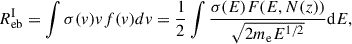
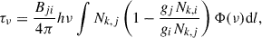
In the optically thin case, the line intensity Iν is the integral from the emissivity over the line of sight (e.g., Mihalas 1978; Pradhan & Nahar 2011)
 (8)
(8)
where emissivity ϵij is the energy emitted in given line per unit volume per unit time, i and j are the atomic levels, ν = hc/λij is the frequency, Aij is the Einstein coefficient for spontaneous emission from level i to level j, and Nk, i is density of k-times ionized atom with electron on the exited level, i. The emissivity can be written as
 (9)
(9)
where Nk is the density of k-times ionized atoms, NSi is the density of all ions of an element (in our case, Si), and NH is hydrogen density. The term Nk, i/Nk is relative population of level i, Nk/NSi is the ratio of k-times ionized ions to total number of silicon ions, and ASi = NSi/NH is silicon abundance.
To calculate the relative level populations of Si IV, we used the full CHIANTI 161-levels model. We also tested a reduced 15-level model and its precision with respect to the full model. The results with the reduced model agreed within 7% with the full model for the range of temperatures and densities typical in the flaring chromosphere and transition region. However, for the final calculation, we used the full 161-level model.
3.3. Optical depth
Given rather high electron densities detected in the flaring transition region, the strong allowed lines, such as Si IV 1402.8 Å, can become optically thick depending on the local plasma conditions. To calculate the optical thickness τ for the Si IV doublet lines at 1402.77 Å and 1393.75 Å, we used the following expression (e.g., Mihalas 1978):
 (10)
(10)
where Bij is Einstein coefficient for absorption, Φ(ν) is an absorption profile, Nk, j is the density of k-times ionized atom with electron on the level, j, and gi and gj are the corresponding statistical weights of levels. The correction for the stimulated emission is given by the term in the brackets.
 |
Fig. 3. Energy deposition [erg cm−3 s−1] for different model runs. Details on the energy fluxes [erg cm−2 s−1], low-energy cutoffs, Emin [keV], and power-law indices, δ, are given in each panel title. |
The absorption profile in the transition region can be approximated by the thermal Doppler profile
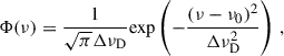 (11)
(11)
where ΔνD is the Doppler line width. The optical thickness in the line center (ν = ν0) can then be expressed as
 (12)
(12)
For Si IV lines 1402.8 Å and 1393.75 Å, the relative populations of the upper levels (Nk, i/Nk, j) are lower than 10−4 and, consequently, the term in the parentheses of Eq. (12) is close to unity. This also means that relative population of the ground level (to which both lines decay) is close to 1 within a similar precision.
The optical thickness depends inversely on the line width. The thermal width of the Si IV lines is relatively small. However, the observed line width of Si IV lines, even outside flares, is of the order of 0.1 Å or larger (see, e.g., Peter et al. 2014; Polito et al. 2016; Dudík et al. 2017); that is, at least about six to seven times wider than their thermal width. Since the optical thickness τ=1 corresponds approximately to the maximum depth from which we can observe radiation, we calculated the altitude (atmospheric height) of the level of τ=1 for three selected cases: for the thermal width, for the width of 0.1 Å (quiet Sun), and for a much larger width of 0.5 Å sometimes reached in flaring plasmas (see, e.g., Lörinčík et al. 2022a,b; Joshi et al. 2025).
4. Results
4.1. Chromospheric response
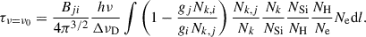
Solar chromosphere reacts on timescales of about 1 s or shorter (Kašparová et al. 2009) to the beam energy deposition (see Sect. 4.4). In all cases, there are notable changes in temperature along the loop even at or before the time the energy deposition reaches its triangular peak. These changes occur even when the peak deposition occurs at t= 1 s (see Fig. 4a). For longer heating durations, the changes in the chromosphere are even more pronounced and occur at even earlier times. For example, if the peak occurs at 3 s, with other beam parameters being the same (top right panel of Fig. 4), there is a notable increase in temperature at heights above ≈1300 km even at 2 s after the start of the heating. At this time and location, the temperature exceeds log(T [K]) = 4.5, and a “hot bubble” is formed.
 |
Fig. 4. Evolution of temperature [K] in different models. Details are given in the titles of panels and the arrangement of panels, parameters, and their units are the same as in Fig. 3. The overplotted contours correspond to isotherms at log(T [K]) = 4.5, 4.7, and 4.9. |
The formation of the hot bubble, characterized by a peak of temperature within the chromosphere (Fig. 4), is a typical result of our simulations with short beam heating durations. These hot bubbles were previously found in RADYN models of Reid et al. (2020) and Carlsson et al. (2023). They represent hot regions of chromospheric plasma heated by the particle beam. Our modeling reproduces the existence of the hot bubble in all studied cases. The hot bubbles are formed relatively high, at 1200–1500 km (see Fig. 4), whereas their formation height corresponds to the position of maximum energy deposition rate (see Fig. 3) and is in agreement with RADYN simulations (Reid et al. 2020; Carlsson et al. 2023). A cutoff at lower energies results in the energy being deposited higher in the atmosphere and, consequently, the hot bubble is also formed at larger heights (see Figs. 3 and 4). Longer beam durations or higher δ result in more extensive hot bubble (compare Fig. 4, panels b and c; panels b and d). If the duration of the electron beam heating is longer, temperature in the region between the bubble and transition region (located at greater heights) increases, trying to form a temperature plateau (Fig. 4b–f). In our simulations, this hot bubble is moving upwards at a velocity of about 10 km s−1. The expansion of chromospheric plasma due to the hot bubble can be seen on the density maps, see Fig. 5). There, the contours correspond to isotherms so that the hot bubble can be easily located (compare Figs. 4 and 5). The plasma density in these hot bubbles is lower than in its surroundings, leading to dilution expanding with time, pushing the overlying denser layers upward with velocity about 10 k ms−1 (see Figs. 5 and 6). In all cases, the lower part of the bubble is pushed downwards (the most visible in Fig. 6e). This behavior of hot bubbles is consistent with RADYN simulations for short-duration energy deposition. Reid et al. (2020) also showed that bubbles move up to the transition region with velocity increasing with duration of the energy deposition by the electron beam.
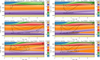 |
Fig. 5. Electron density [cm−3] for different models. Details are given in the titles of panels and the arrangement of panels, parameters, and their units are the same as in Fig. 3. The overplotted contours correspond to isotherms at log(T [K]) = 4.5, 4.7, and 4.9. |
 |
Fig. 6. Temporal behavior of velocity [kms−1] for different models. Details are given in the title of panels and the arrangement of panels, parameters, and their units are the same as in Fig. 4. Black contours show Si IV reference emissivity at level 0.1 and 0.01 of its maximum. |
4.2. Si IV emission and non-equilibrium effects
The emissivities of the Si IV 1402.8 Å line, calculated including the non-equilibrium ionization, suppression of dielectronic recombination, as well as ionization and excitation by the electron beam, are shown in Fig. 7. The emissivities are plotted in a logarithmic scale. For optically thin plasma and electron beams with short duration, the main contributions to the emissivity (by several orders of magnitude) originate in the hot bubble itself.
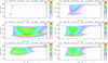 |
Fig. 7. Temporal behavior of Si IV 1402.8 Å line emissivity [phot cm−3 sr−1 s−1] for different models. Details are given in the titles of panels and the arrangement of panels, parameters, and their units are the same as in Fig. 3. |
These emissivities, with all effects included, are used as reference emissivities for the estimation of the importance of individual effects on the Si IV emissivity. For this purpose, a particular process is omitted from the calculation and the result is compared to the reference emissivity.
The importance of non-equilibrium ionization in various regions of the flaring atmosphere can be seen in Fig. 8. This figure shows the ratio of the Si IV ionization fraction calculated using Eq. (1) to those calculated under the assumption of the ionization equilibrium. The ratio of the non-equilibrium Si IV ionization fractions with respect to the equilibrium ones varies between 0.05 and 70 and in Fig. 8 it is displayed only where the relative Si IV abundance is higher than 0.01; that is, in regions where the Si IV is formed. It is thus clear that non-equilibrium ionization is important. Figure 8 demonstrates that the ionization state is not able to follow changes in temperature during the fast heating and cooling. For temperatures below the temperature corresponding to the ionization peak of Si IV in equilibrium, non-equilibrium abundance of Si IV are lower than equilibrium abundance during the heating, while they are higher if the plasma is cooling. Inverse behavior can be seen for temperatures above the temperature log(T [K]) = 4.8 corresponding to the Si IV ionization peak in equilibrium for an electron density of ≈1012 cm−3.
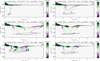 |
Fig. 8. Ratio of Si IV abundances calculated with the assumption of the non-equilibrium ionization to equilibrium abundances. The ratio is showed for where the relative Si IV abundance out of equilibrium is higher than 0.01. Details are given in the title of panels and the arrangement of the panels, parameters, and their units are the same as in Fig. 3. |
Figure 9 shows the effect of beam ionization and excitation on the evolution of the Si IV emissivities. This figure shows the ratio of the Si IV emissivities calculated with and without ionization and excitation by the electron beam. The effect of the suppression of the dielectronic recombination was included. The contours of theSi IV emissivity correspond to the 0.1 and 0.01 levels with respect to its maxima for the case where the beam ionization and excitation are included.
The highest contribution of the beam ionization rate to the total ionization rate (green color regions) comes from the boundary regions with low emissivity (< 0.01) and temperature below log(T [K]) = 4.7; that is, below the peak of the Si IV relative ion abundance in equilibrium. This holds for five out of the six studied cases. An exception is the case of Fig. 9b, where the electron beam increases the Si IV emissivity in the region between relative contours 0.1 and 0.01. This means that the effect of the beam cannot always be neglected.
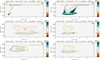 |
Fig. 9. Ratio of the Si IV 1402.8 Å emissivity calculated with the contribution of the electron beam to both ionization and excitation with respect to the emissivity without the beam contribution. Black contours show the reference emissivity at level 0.1 and 0.01 of its maximum. The arrangement of the panels, parameters, and their units are the same as in Fig. 3. |
The overall small decrease of emissivity due to the electron beam in regions of the highest emissivity comes from the changes in excitation. Presence of electron beam particles increases the excitation rates from the upper energy levels of Si IV 1394 Å and 1403 Å lines, which leads to a small decrease in the population of levels these lines originate from.
4.3. Suppression of dielectronic recombination
The effect of the suppression of the dielectronic recombination is shown in Fig. 10. The green and violet colors correspond to regions where the suppression of dielectronic recombination leads to higher or lower Si IV emissivities, with respect to the case when the dielectronic suppression is not accounted for. The black contours again denote the Si IV reference emissivity at 0.1 and 0.01 level with included dielectronic suppression. It is immediately seen that the regions where the Si IV is dominantly formed correspond to those where the suppression of dielectronic recombination leads to strong enhancements (up to an order of magnitude) in the Si IV emissivity. This is because lower dielectronic recombination rates result in longer lifetimes for all the ions; therefore, the Si IV ions can exist and emit for a longer time. This means that the effect of the suppression of dielectronic recombination is significant in the context of solar flares, and should not be neglected
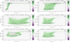 |
Fig. 10. Ratio of the Si IV 1402.8 Å reference emissivity calculated with density suppression of the dielectronic recombination to the emissivity without this suppression. Black contours show reference emissivity at level 0.1 and 0.01 of its maximum. |
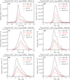 |
Fig. 11. Time evolution of total Si IV 1402.77 Å intensity calculated assuming optically thin plasma and for different models. Details are given in the titles of panels and the arrangement of the panels, parameters, and their units is the same as in Fig. 3. Black lines correspond to the Si 1393.75 Å line and red lines to the 1402.77 Å line. Dashed lines show total intensities calculated without density suppression of dielectronic recombination. |
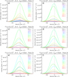 |
Fig. 12. Time evolution of Si IV 1402.77 Å line profile calculated for optically thin case and for different models. Details are given in the title of panels and the arrangement of panels, parameters, and their units are the same as in Fig. 4. Time increases from black-blue-green-yellow to red. The mean profile is plotted by a black dashed line. |
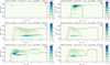 |
Fig. 13. Changes of Δτ per 10 km for different models. Details are given in the title of panels and the arrangement of panels, parameters, and their units are the same as in Fig. 3. Thick black contour shows level τ = 1 for thermal Doppler width, a thin black line for 0.1 Å Doppler width and a grey line for 0.5 Å. Labels on the left side of the color scale correspond to thermal width and on the right side to 0.1 Å. |
References
- Abbett, W. P., & Hawley, S. L. 1999, ApJ, 521, 906 [NASA ADS] [CrossRef] [Google Scholar]
- Allred, J. C., Hawley, S. L., Abbett, W. P., & Carlsson, M. 2005, ApJ, 630, 573 [NASA ADS] [CrossRef] [Google Scholar]
- Allred, J. C., Kowalski, A. F., & Carlsson, M. 2015, ApJ, 809, 104 [NASA ADS] [CrossRef] [Google Scholar]
- Aschwanden, M. J., Schwartz, R. A., & Alt, D. M. 1995, ApJ, 447, 923 [NASA ADS] [CrossRef] [Google Scholar]
- Aulanier, G., Pariat, E., Démoulin, P., & Devore, C. R. 2006, Sol. Phys., 238, 347 [NASA ADS] [CrossRef] [Google Scholar]
- Aulanier, G., Janvier, M., & Schmieder, B. 2012, A&A, 543, A110 [NASA ADS] [CrossRef] [EDP Sciences] [Google Scholar]
- Babu, B. S., Kayshap, P., Tripathi, S. C., Jelínek, P., & Dwivedi, B. N. 2024, MNRAS, 528, 2474 [NASA ADS] [CrossRef] [Google Scholar]
- Benz, A. O. 2008, Liv. Rev. Sol. Phys., 5, 1 [Google Scholar]
- Bradshaw, S. J., & Mason, H. E. 2003a, A&A, 401, 699 [NASA ADS] [CrossRef] [EDP Sciences] [Google Scholar]
- Bradshaw, S. J., & Mason, H. E. 2003b, A&A, 407, 1127 [NASA ADS] [CrossRef] [EDP Sciences] [Google Scholar]
- Brosius, J. W. 2009, ApJ, 701, 1209 [Google Scholar]
- Brown, J. C. 1971, Sol. Phys., 18, 489 [Google Scholar]
- Brown, J. C. 1972, Sol. Phys., 26, 441 [NASA ADS] [CrossRef] [Google Scholar]
- Burgess, A., & Summers, H. P. 1969, ApJ, 157, 1007 [NASA ADS] [CrossRef] [Google Scholar]
- Carlsson, M., & Stein, R. F. 1992, ApJ, 397, L59 [Google Scholar]
- Carlsson, M., & Stein, R. F. 1997, ApJ, 481, 500 [Google Scholar]
- Carlsson, M., Fletcher, L., Allred, J., et al. 2023, A&A, 673, A150 [NASA ADS] [CrossRef] [EDP Sciences] [Google Scholar]
- Cheng, C. C., Bruner, E. C., Tandberg-Hanssen, E., et al. 1982, ApJ, 253, 353 [Google Scholar]
- Cheng, J. X., Qiu, J., Ding, M. D., & Wang, H. 2012, A&A, 547, A73 [NASA ADS] [CrossRef] [EDP Sciences] [Google Scholar]
- De Pontieu, B., Title, A. M., Lemen, J. R., et al. 2014, Sol. Phys., 289, 2733 [Google Scholar]
- Del Zanna, G., Dere, K. P., Young, P. R., & Landi, E. 2021, ApJ, 909, 38 [NASA ADS] [CrossRef] [Google Scholar]
- Dere, K. P., Landi, E., Mason, H. E., Monsignori Fossi, B. C., & Young, P. R. 1997, A&AS, 125, 149 [NASA ADS] [CrossRef] [EDP Sciences] [Google Scholar]
- Dudík, J., Del Zanna, G., Dzifčáková, E., Mason, H. E., & Golub, L. 2014a, ApJ, 780, L12 [Google Scholar]
- Dudík, J., Janvier, M., Aulanier, G., et al. 2014b, ApJ, 784, 144 [CrossRef] [Google Scholar]
- Dudík, J., Polito, V., Janvier, M., et al. 2016, ApJ, 823, 41 [Google Scholar]
- Dudík, J., Polito, V., Dzifčáková, E., Del Zanna, G., & Testa, P. 2017, ApJ, 842, 19 [CrossRef] [Google Scholar]
- Emslie, A. G. 1978, ApJ, 224, 241 [NASA ADS] [CrossRef] [Google Scholar]
- García-Rivas, M., Kašparová, J., Berlicki, A., et al. 2024, A&A, 690, A254 [NASA ADS] [CrossRef] [EDP Sciences] [Google Scholar]
- Holman, G. D., Aschwanden, M. J., Aurass, H., et al. 2011, Space Sci. Rev., 159, 107 [NASA ADS] [CrossRef] [Google Scholar]
- Hoyng, P., Brown, J. C., & van Beek, H. F. 1976, Sol. Phys., 48, 197 [Google Scholar]
- Hudson, H. S., Strong, K. T., Dennis, B. R., et al. 1994, ApJ, 422, L25 [Google Scholar]
- Janvier, M., Aulanier, G., Pariat, E., & Démoulin, P. 2013, A&A, 555, A77 [NASA ADS] [CrossRef] [EDP Sciences] [Google Scholar]
- Jeffrey, N. L. S., Fletcher, L., Labrosse, N., & Simões, P. J. A. 2018, Sci. Adv., 4, 2794 [Google Scholar]
- Joshi, R., Dudík, J., Schmieder, B., Aulanier, G., & Chandra, R. 2025, A&A, 698, A301 [NASA ADS] [CrossRef] [EDP Sciences] [Google Scholar]
- Kašparová, J., Varady, M., Heinzel, P., Karlický, M., & Moravec, Z. 2009, A&A, 499, 923 [NASA ADS] [CrossRef] [EDP Sciences] [Google Scholar]
- Kašparová, J., Carlsson, M., Heinzel, P., & Varady, M. 2019, in Radiative Signatures from the Cosmos, eds. K. Werner, C. Stehle, T. Rauch, & T. Lanz, ASP Conf. Ser., 519, 141 [Google Scholar]
- Kerr, G. S. 2022, Front. Astron. Space Sci., 9, 1060856 [NASA ADS] [CrossRef] [Google Scholar]
- Kerr, G. S., Carlsson, M., Allred, J. C., Young, P. R., & Daw, A. N. 2019, ApJ, 871, 23 [NASA ADS] [CrossRef] [Google Scholar]
- Kiplinger, A. L., Dennis, B. R., Frost, K. J., Orwig, L. E., & Emslie, A. G. 1983, ApJ, 265, L99 [Google Scholar]
- Knuth, T., & Glesener, L. 2020, ApJ, 903, 63 [NASA ADS] [CrossRef] [Google Scholar]
- Li, T., & Zhang, J. 2014, ApJ, 791, L13 [NASA ADS] [CrossRef] [Google Scholar]
- Li, T., & Zhang, J. 2015, ApJ, 804, L8 [NASA ADS] [CrossRef] [Google Scholar]
- Li, Y., Ding, M. D., Qiu, J., & Cheng, J. X. 2015, ApJ, 811, 7 [NASA ADS] [CrossRef] [Google Scholar]
- Li, T., Yang, K., Hou, Y., & Zhang, J. 2016, ApJ, 830, 152 [CrossRef] [Google Scholar]
- Li, Y., Kelly, M., Ding, M. D., et al. 2017, ApJ, 848, 118 [Google Scholar]
- Li, Y., Ding, M. D., Hong, J., Li, H., & Gan, W. Q. 2019, ApJ, 879, 30 [NASA ADS] [CrossRef] [Google Scholar]
- Lörinčík, J., Aulanier, G., Dudík, J., Zemanová, A., & Dzifčáková, E. 2019, ApJ, 881, 68 [Google Scholar]
- Lörinčík, J., Dudík, J., & Polito, V. 2022a, ApJ, 934, 80 [CrossRef] [Google Scholar]
- Lörinčík, J., Polito, V., De Pontieu, B., Yu, S., & Freij, N. 2022b, Front. Astron. Space Sci., 9, 334 [Google Scholar]
- Lörinčík, J., Dudík, J., Sainz Dalda, A., et al. 2025, Nat. Astron., 9, 45 [Google Scholar]
- Mihalas, D. 1978, Stellar Atmospheres (San Francisco: W.H. Freeman) [Google Scholar]
- Milligan, R. O., Gallagher, P. T., Mathioudakis, M., & Keenan, F. P. 2006, ApJ, 642, L169 [NASA ADS] [CrossRef] [Google Scholar]
- Nagai, F., & Emslie, A. G. 1984, ApJ, 279, 896 [Google Scholar]
- Nikolić, D., Gorczyca, T. W., Korista, K. T., Ferland, G. J., & Badnell, N. R. 2013, ApJ, 768, 82 [CrossRef] [Google Scholar]
- Nikolić, D., Gorczyca, T. W., Korista, K. T., et al. 2018, ApJS, 237, 41 [CrossRef] [Google Scholar]
- Olluri, K., Gudiksen, B. V., & Hansteen, V. H. 2013, ApJ, 767, 43 [NASA ADS] [CrossRef] [Google Scholar]
- Peter, H., Tian, H., Curdt, W., et al. 2014, Science, 346, 1255726 [Google Scholar]
- Polito, V., Del Zanna, G., Dudík, J., et al. 2016, A&A, 594, A64 [NASA ADS] [CrossRef] [EDP Sciences] [Google Scholar]
- Polito, V., Testa, P., Allred, J., et al. 2018, ApJ, 856, 178 [NASA ADS] [CrossRef] [Google Scholar]
- Pradhan, A. K., & Nahar, S. N. 2011, Atomic Astrophysics and Spectroscopy (Cambridge University Press) [Google Scholar]
- Qiu, J., Cheng, J. X., Hurford, G. J., Xu, Y., & Wang, H. 2012, A&A, 547, A72 [NASA ADS] [CrossRef] [EDP Sciences] [Google Scholar]
- Radziszewski, K., Heinzel, P., Kašparová, J., et al. 2024, ApJ, 977, 132 [Google Scholar]
- Reep, J. W., Warren, H. P., Crump, N. A., & Simões, P. J. A. 2016, ApJ, 827, 145 [Google Scholar]
- Reep, J. W., Russell, A. J. B., Tarr, L. A., & Leake, J. E. 2018, ApJ, 853, 101 [NASA ADS] [CrossRef] [Google Scholar]
- Reid, A., Zhigulin, B., Carlsson, M., & Mathioudakis, M. 2020, ApJ, 894, L21 [NASA ADS] [CrossRef] [Google Scholar]
- Rubio da Costa, F., Liu, W., Petrosian, V., & Carlsson, M. 2015, ApJ, 813, 133 [Google Scholar]
- Smith, R. K., & Hughes, J. P. 2010, ApJ, 718, 583 [NASA ADS] [CrossRef] [Google Scholar]
- Sobotka, M., Dudík, J., Denker, C., et al. 2016, A&A, 596, A1 [Google Scholar]
- Tandberg-Hanssen, E., Reichmann, E., & Woodgate, B. 1983, Sol. Phys., 86, 159 [Google Scholar]
- Testa, P., De Pontieu, B., Allred, J., et al. 2014, Science, 346, 1255724 [Google Scholar]
- Tian, H., Young, P. R., Reeves, K. K., et al. 2015, ApJ, 811, 139 [NASA ADS] [CrossRef] [Google Scholar]
- Tripathi, D., Nived, V. N., Isobe, H., & Doyle, G. G. 2020, ApJ, 894, 128 [CrossRef] [Google Scholar]
- Varady, M., Kasparova, J., Moravec, Z., Heinzel, P., & Karlicky, M. 2010, IEEE Trans. Plasma Sci., 38, 2249 [CrossRef] [Google Scholar]
- Vernazza, J. E., Avrett, E. H., & Loeser, R. 1981, ApJS, 45, 635 [Google Scholar]
- Warren, H. P., Reep, J. W., Crump, N. A., & Simões, P. J. A. 2016, ApJ, 829, 35 [Google Scholar]
- Yan, L., Peter, H., He, J., et al. 2015, ApJ, 811, 48 [NASA ADS] [CrossRef] [Google Scholar]
- Zhou, Y.-A., Hong, J., Li, Y., & Ding, M. D. 2022, ApJ, 926, 223 [NASA ADS] [CrossRef] [Google Scholar]
- Zhou, Y., Yan, X., Xue, Z., et al. 2024, A&A, 692, A210 [NASA ADS] [CrossRef] [EDP Sciences] [Google Scholar]
All Figures
|
Fig. 1. Temperature (black line) and electron density (red dashed line) in the initial VAL C atmosphere. |
| In the text | |
|
Fig. 2. Triangular flux modulation with the peak at 5 s. |
| In the text | |
|
Fig. 3. Energy deposition [erg cm−3 s−1] for different model runs. Details on the energy fluxes [erg cm−2 s−1], low-energy cutoffs, Emin [keV], and power-law indices, δ, are given in each panel title. |
| In the text | |
|
Fig. 4. Evolution of temperature [K] in different models. Details are given in the titles of panels and the arrangement of panels, parameters, and their units are the same as in Fig. 3. The overplotted contours correspond to isotherms at log(T [K]) = 4.5, 4.7, and 4.9. |
| In the text | |
|
Fig. 5. Electron density [cm−3] for different models. Details are given in the titles of panels and the arrangement of panels, parameters, and their units are the same as in Fig. 3. The overplotted contours correspond to isotherms at log(T [K]) = 4.5, 4.7, and 4.9. |
| In the text | |
|
Fig. 6. Temporal behavior of velocity [kms−1] for different models. Details are given in the title of panels and the arrangement of panels, parameters, and their units are the same as in Fig. 4. Black contours show Si IV reference emissivity at level 0.1 and 0.01 of its maximum. |
| In the text | |
|
Fig. 7. Temporal behavior of Si IV 1402.8 Å line emissivity [phot cm−3 sr−1 s−1] for different models. Details are given in the titles of panels and the arrangement of panels, parameters, and their units are the same as in Fig. 3. |
| In the text | |
|
Fig. 8. Ratio of Si IV abundances calculated with the assumption of the non-equilibrium ionization to equilibrium abundances. The ratio is showed for where the relative Si IV abundance out of equilibrium is higher than 0.01. Details are given in the title of panels and the arrangement of the panels, parameters, and their units are the same as in Fig. 3. |
| In the text | |
|
Fig. 9. Ratio of the Si IV 1402.8 Å emissivity calculated with the contribution of the electron beam to both ionization and excitation with respect to the emissivity without the beam contribution. Black contours show the reference emissivity at level 0.1 and 0.01 of its maximum. The arrangement of the panels, parameters, and their units are the same as in Fig. 3. |
| In the text | |
|
Fig. 10. Ratio of the Si IV 1402.8 Å reference emissivity calculated with density suppression of the dielectronic recombination to the emissivity without this suppression. Black contours show reference emissivity at level 0.1 and 0.01 of its maximum. |
| In the text | |
|
Fig. 11. Time evolution of total Si IV 1402.77 Å intensity calculated assuming optically thin plasma and for different models. Details are given in the titles of panels and the arrangement of the panels, parameters, and their units is the same as in Fig. 3. Black lines correspond to the Si 1393.75 Å line and red lines to the 1402.77 Å line. Dashed lines show total intensities calculated without density suppression of dielectronic recombination. |
| In the text | |
|
Fig. 12. Time evolution of Si IV 1402.77 Å line profile calculated for optically thin case and for different models. Details are given in the title of panels and the arrangement of panels, parameters, and their units are the same as in Fig. 4. Time increases from black-blue-green-yellow to red. The mean profile is plotted by a black dashed line. |
| In the text | |
|
Fig. 13. Changes of Δτ per 10 km for different models. Details are given in the title of panels and the arrangement of panels, parameters, and their units are the same as in Fig. 3. Thick black contour shows level τ = 1 for thermal Doppler width, a thin black line for 0.1 Å Doppler width and a grey line for 0.5 Å. Labels on the left side of the color scale correspond to thermal width and on the right side to 0.1 Å. |
| In the text | |
Current usage metrics show cumulative count of Article Views (full-text article views including HTML views, PDF and ePub downloads, according to the available data) and Abstracts Views on Vision4Press platform.
Data correspond to usage on the plateform after 2015. The current usage metrics is available 48-96 hours after online publication and is updated daily on week days.
Initial download of the metrics may take a while.