| Issue |
A&A
Volume 702, October 2025
|
|
|---|---|---|
| Article Number | A104 | |
| Number of page(s) | 11 | |
| Section | Stellar structure and evolution | |
| DOI | https://doi.org/10.1051/0004-6361/202556149 | |
| Published online | 10 October 2025 | |
EL CMi: Confirmation of triaxial pulsation theory
1
Nicolaus Copernicus Astronomical Center, Polish Academy of Sciences, ul. Bartycka 18, PL-00-716 Warszawa, Poland
2
Department of Physics and Kavli Institute for Astrophysics and Space Research, Massachusetts Institute of Technology, 77 Massachusetts Ave, Cambridge, MA 02139, USA
3
Instituto de Astrofísica de Canarias, 38205 La Laguna, Spain
4
Departamento de Astrofísica, Universidad de la Laguna, 38206 La Laguna, Tenerife, Spain
5
Citizen Scientist, c/o Zooniverse, Dept., of Physics, University of Oxford, Denys Wilkinson Building, Keble Road, Oxford OX1 3RH, UK
6
Amateur Astronomer, Glendale, AZ 85308, USA
7
TAPIR, Mailcode 350-17, California Institute of Technology, Pasadena, CA 91125, USA
8
Centre for Space Research, North-West University, Mahikeng 2745, South Africa
9
Jeremiah Horrocks Institute, University of Central Lancashire, Preston PR1 2HE, UK
10
Department of Physics, Gibbet Hill Road, University of Warwick, Coventry CV4 7AL, UK
11
Yunnan Observatories, Chinese Academy of Sciences (CAS), Kunming 650216, PR China
12
International Centre of Supernovae, Yunnan Key Laboratory, Kunming 650216, PR China
13
NASA Goddard Space Flight Center, 8800 Greenbelt Road, Greenbelt, MD 20771, USA
14
SETI Institute, 189 Bernardo Ave, Suite 200, Mountain View, CA 94043, USA
⋆ Corresponding author: This email address is being protected from spambots. You need JavaScript enabled to view it.
Received:
27
June 2025
Accepted:
27
July 2025
Abstract
Triaxial pulsators are a recently discovered group of oscillating stars in close binary systems that pulsate around three axes at the same time. It has recently been theoretically shown that new types of pulsation modes, the tidally tilted standing (TTS) modes, can arise in these stars. We report the first detection of a quadrupole TTS oscillation mode in the pulsating component of the binary system EL CMi following an analysis of TESS space photometry. Two dipole oscillations around different axes in the orbital plane are present as well. In addition, we characterize the binary system using new radial velocity measurements and PHOEBE as well as simultaneous spectral energy distribution and light curve modeling. The pulsating primary component has properties typical of a δ Scuti star, but has accreted and is still accreting mass from its Roche-lobe filling companion. The donor star is predicted to evolve into a low-mass helium white dwarf. EL CMi demonstrates the potential of asteroseismic inferences of the structure of stars in close binaries before and after mass transfer and in three spatial dimensions.
Key words: binaries: close / binaries: eclipsing / binaries: spectroscopic / stars: evolution / stars: oscillations / stars: variables: δ Scuti
© The Authors 2025
 Open Access article, published by EDP Sciences, under the terms of the Creative Commons Attribution License (https://creativecommons.org/licenses/by/4.0), which permits unrestricted use, distribution, and reproduction in any medium, provided the original work is properly cited.
This article is published in open access under the Subscribe to Open model. This email address is being protected from spambots. You need JavaScript enabled to view it. to support open access publication.
1. Introduction
The development of high-precision photometric space missions such as Convection Rotation and Planetary Transits (CoRoT) (Baglin et al. 2006), Kepler (Koch et al. 2010), Transiting Exoplanet Survey Satellite (TESS) (Ricker et al. 2015), CHaracterising ExOPlanets Satellite (CHEOPS) (Benz et al. 2021), and PLAnetary Transits and Oscillations of stars (PLATO) (Rauer et al. 2014) was primarily motivated by the quest for extrasolar planets by detecting transits and for the characterization of these planets. In addition to the orbital inclination and information on the limb darkening, however, the transit method just yields the ratio of the planetary to stellar radius. To determine absolute dimensions, knowledge about the size of the planetary host star is required.
This is where asteroseismology comes into play. Asteroseismology determines the interior structure of stars by using stellar oscillations as seismic waves (e.g., Aerts 2021; Kurtz 2022, and references therein) and is at the same time capable of constraining the absolute parameters of its target stars (e.g., Huber et al. 2013). As asteroseismic investigations themselves also greatly benefit from high-accuracy photometric data, almost all of the planet-search space missions have an asteroseismology program as well (e.g., Gilliland et al. 2010).
The outcome from those missions in terms of asteroseismic research has been rich. To mention just a few results from TESS alone, more than 150 000 oscillating red giant (Hon et al. 2021) and over 100 000 pulsating A–F type stars (Gootkin et al. 2024) have been discovered, period-spacing patterns were detected that permitted asteroseismology of dozens of δ Scuti stars for the first time (Bedding et al. 2020), low-frequency oscillations in massive supergiant stars appear to be ubiquitous (Bowman et al. 2019), and the interiors of individual massive stars were studied (Burssens et al. 2023).
The availability of data of unprecedented quality clearly also facilitated the discovery of unexpected phenomena, such as a star that stopped to pulsate (Kurtz et al. 2025), or stars in close binary systems whose pulsation axes are tilted with respect to their rotation axes through the gravitational pull of their companion star (Handler et al. 2020). Several more of these systems were reported soon afterwards (Kurtz et al. 2020; Rappaport et al. 2021; Kahraman Aliçavuş et al. 2022; Jennings et al. 2024). Whereas the pulsating star in the latter binaries was of the δ Scuti type, a tidally tilted subdwarf B pulsator was also discovered (Jayaraman et al. 2022a). From the point of view of theory, the pulsations of these objects were explained via tidal mode coupling that both tilts the pulsation axes and confines the pulsations to certain regions of the star (Fuller et al. 2020).
More recently, two of the tidally tilted pulsators have been found to be triaxial pulsators with dipole pulsations about three orthogonal axes, including the tidal axis (Zhang et al. 2024; Jayaraman et al. 2024). Based on these discoveries, Fuller et al. (2025) developed a theoretical description of how these modes of pulsation may appear in triaxially deformed stars. Henceforth, these are called tidally tilted standing modes (TTS; sometimes Fuller modes for short). These are modes that arise when tidal, centrifugal, and Coriolis perturbations couple modes of equal spherical degrees (Fuller et al. 2025). These modes were found to be triaxial for dipole configurations, while for higher multipole modes, their geometry is more complex. These modes typically receive nearly equal contributions from spherical harmonics of spherical degrees +m and −m, which means that the modes are primarily standing modes that do not propagate around the rotation axis. Instead, their pattern is nearly stationary with respect to the companion star.
Furthermore, based on this theory, Fuller et al. (2025) predicted how quadrupole triaxial pulsation modes would manifest themselves observationally and provided the theoretical expressions for quadrupole and octupole TTS pulsations. We report the discovery of a textbook example of a pulsator with two dipole modes around different axes in the orbital plane plus a quadrupole Fuller mode that occurs in the primary component of the eclipsing binary system EL CMi.
2. Observations and analysis
2.1. Photometry
The source EL CMi (TIC 321254859) has been observed with TESS in full-frame images taken during Sectors 7 (January 2019), 34 (January 2021), 61 (February 2023), and 88 (January 2025) with cadences of 1800, 600, 200, and 200 s, respectively. TESS-SPOC light curves are available for the first two sectors, and we made our own lightkurve reductions for the Sector 61 and 88 data. All light curves show some drifts in the mean brightness that were filtered out, and we removed segments with poor data quality. EL CMi was initially identified as the high-scoring output of a neural network that was designed to find eclipses in TESS light curves. This is described further in Powell et al. (2021) and Kostov et al. (2025). Upon manual review, tidally tilted or triaxial pulsations were suspected in the Sector 61 data. Consequently, the system was subjected to closer examination regarding the periodic content in its light curves.
To perform frequency analyses, we used the software package Period04 (Lenz & Breger 2005). This package applies Fourier analysis and simultaneous multifrequency sine-wave fitting. Advanced options such as the calculation of optimal light-curve fits for multiperiodic signals including harmonic, combination, and equally spaced frequencies are available. Fits composed of multiple sine waves were subtracted from the data, and the residuals were examined for further periodicities.
TESS data come in different flavors, in particular, simple aperture photometry (SAP; Twicken et al. 2010; Morris et al. 2020) and pre-search data conditioning SAP (PDCSAP; Stumpe et al. 2012; Smith et al. 2012) fluxes. The latter were detrended using co-trending basis vectors and are often cleaner than SAP fluxes. On the other hand, the detrending procedure can distort light curves with intrinsic sharp features, such as eclipses, and the choice of the optimal data version therefore sometimes depends on the goals and demands of the scientific analysis to be carried out.
The eclipses in the Sector 7 and 34 SAP data for EL CMi appear to be shallower than in the PDCSAP and in the Sector 61 and 88 data. This can be explained by blending of nearby stars into the photometric apertures, as implied by the corresponding CROWDSAP parameters (0.8784 and 0.8959). Therefore, the analysis of the binary light curve was based on the Sector 34 PDCSAP data, which are expected to no longer be contaminated by the companion. On the other hand, the Fourier noise level in the range of the pulsation frequencies is considerably lower (by about 30%) in the SAP data than in the PDCSAP light curves. Consequently, the SAP data were used to detect the pulsational frequencies, with the caveat that their amplitudes may be systematically lower than in reality. This is not relevant for the results of the analyses performed on these data, however.
In a first step, the ephemeris for the times of primary minimum from the TESS data was determined by computing a multiharmonic fit to the light curves merged into 1800 s bins to give them all equal weight. This ephemeris was

where the zeropoint in time relates to the center of the first primary eclipse in the Sector 34 data. The corresponding orbital phase curve is shown in Fig. 1.
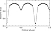 |
Fig. 1. Phase-folded TESS Sector 34 PDCSAP light curve of EL CMi without the pulsation. |
Only the Sector 34, 61 and 88 data were used to analyze the pulsations because the pulsation frequencies are above the Nyquist limit of the Sector 7 data. An essential question in the quest for the detection of periodic signals in a dataset is where to stop the analysis. To this end, several criteria have been proposed. We adopted the method that was originally put forward by Breger et al. (1993). In this framework, a Fourier peak must exceed the mean amplitude in the amplitude spectrum by a factor of 4 in the local frequency domain to be considered significant. For space-based data, this can lead to an overinterpretation of the periodic content, however (Balona 2014). For TESS data, Baran & Koen (2021) have proposed stricter detection criteria depending on the sampling of the dataset. Interpolating their values, we adopted thresholds with a signal-to-noise ratio (S/N) of 4.8 for the Sector 34 data and of 5.0 for the Sector 61 and 88 data. They correspond to false-alarm probabilities of 0.1%. The mean amplitude of the noise was evaluated in a 5 d−1 wide window centered at the frequency under consideration.
We detected the pulsation frequencies based on the residuals of a multiharmonic fit accounting for the eclipses. We then added the pulsation frequencies to a fit that simultaneously included the eclipses and the pulsations. When no significant signals were left, this process was stopped. At this point, an échelle diagram was constructed with respect to the orbital frequency (see Jayaraman et al. 2022a, for more details) to evaluate which of the detected signals form multiplets. The frequencies of confirmed multiplet members were then fixed to their predicted values using the orbital frequency, and the fit to the complete light curve was optimized and re-evaluated to verify that no additional signals had been left behind. The resulting lists of frequencies are given in Table 1, and the resulting échelle diagram is shown in the upper panel of Fig. 2. The pre-whitening process is illustrated in Fig. 3.
Pulsation-related frequencies of TIC 321254859, that is, EL CMi.
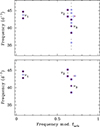 |
Fig. 2. Échelle diagram for EL CMi from Sectors 34 (black), 61 (red), and 88 (blue). Top: All data. Bottom: Primary eclipses removed from the light curve. The sizes of the plot symbols relate to the logarithm of the pulsation amplitude; the cross marks the expected location of the centroid of mode ν2. |
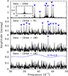 |
Fig. 3. Fourier transforms of the Sector 34 TESS data for EL CMi with subsequent pre-whitening steps (first, only the orbital harmonics, then the orbital harmonics plus 7, 18, and 19 pulsation frequencies indicated by the blue arrows, respectively). The inset in the top panel shows the spectral window function of this dataset. The level of the S/N curve is applicable for all of these amplitude spectra, but is plotted only once for clarity. |
The échelle diagram derived in this way is fairly simple, but shows a faint extended ridge around mode ν3 (Fig. 2, upper panel). This is a sign of spatial filtering (eclipse mapping), which is a known phenomenon among pulsating stars in eclipsing binaries. In brief, when part of the surface of a nonradially pulsating star is covered during an eclipse, only the light variations in the visible part of the star can be measured. This modifies the observed pulsation amplitudes and phases depending on the types of the pulsation modes that are excited (e.g., Van Reeth et al. 2023; Bókon et al. 2025, and references therein).
The effect of spatial filtering occurs when the pulsating star is attenuated by its companion; when the pulsator blocks some light of the constant star, only the background light changes in strength. For this reason, the frequency analysis was repeated using light curves without the primary, and then without the secondary eclipses. As there was no change in the derived set of pulsation frequencies in the latter case, the hotter component of the binary was identified as the pulsator. Figure 4 shows the frequency analysis after the primary eclipses were removed from the Sector 34 data. The list of pulsation-related frequencies derived from all sectors (with sufficient cadence) without the primary eclipses is given in Table 2, and the corresponding échelle diagram can be found in Fig. 2 (lower panel). The results from each individual sector are highly consistent when we acknowledge that the pulsation amplitudes are somewhat variable over time. This precludes the detection of some of the weaker signals in Sectors 61 and 88.
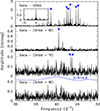 |
Fig. 4. Same as Fig. 3, but for the data without the primary eclipses. The inset in the top panel shows the spectral window function of this dataset. |
Same as Table 1, but from the data without the primary eclipse.
With this information in hand, the runs of pulsation amplitude and phase for the three dominant modes were reconstructed using the method described by Jayaraman et al. (2022a) (their Sect. 3.2). Figure 5 shows the results.
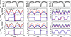 |
Fig. 5. Run of the pulsation amplitude and phase for the three main modes of EL CMi. Black: Sector 34 data. Red: Sector 61 data. Blue: Sector 88 data. Upper panel: Orbital light curve. Second and third panels: All data. Lower two panels: Reconstructions from the data without the primary eclipses. The frequencies are for the multiplet centroids. |
Whereas the amplitudes of the three pulsation modes varied from one sector of data to the next, the runs of the pulsational phases over the orbit were essentially identical. The higher amplitude of ν3 and lower noise level in Sector 34 make the effects of spatial filtering during primary eclipse detectable, whereas there are only indications of this effect in the Sector 88 data, and they are lost in the observational noise in Sector 61. To identify the pulsation modes by comparison with the pulsation amplitude and phase curves theoretically predicted by Fuller et al. (2025), it is more convenient to use the reconstructions from the data without the primary eclipses.
The amplitude and phase modulation of mode ν1 over the orbit is consistent with that of a Y10x dipole mode, whereas the run of mode ν2 is that of a Y10y dipole mode (see Fuller et al. (2025) for visualizations of these modes). These modes were reported previously (Zhang et al. 2024; Jayaraman et al. 2024). The behavior of the pulsation amplitude and phase depending on orbital phase is clearly different for mode ν3; it is that of a quadrupole Y22− mode, which is thus observationally detected for the first time.
As discussed by Fuller et al. (2025), the Y22− mode is a superposition of Y2 + 2z and Y2 − 2z modes. This behaves like an l = m = 2 pattern that is wrapped around the z-axis, with maxima and minima offset from the tidal axis by an angle of π/4, and it is a standing mode that does not propagate around the z-axis.
2.2. Spectroscopy
Spectroscopic observations of EL CMi were carried out with the Alhambra Faint Object Spectrograph and Camera (ALFOSC) instrument in spectroscopy mode at the 2.56 m Nordic Optical Telescope (NOT) on the Observatorio del Roque de los Muchachos, La Palma, Spain, during the nights from 2025 January 23/24 to 27/28. Grism 18 was used and resulted in a wavelength coverage of 3450–5350 Å with a spectral resolution of 2000 using a 0.5″ slit. Integration times of 300 s were used and resulted in a S/N of 65–145 around 4500 Å, depending on weather conditions. Each observation consisted of two or three consecutive integrations.
The data were reduced with the package PypeIt (Prochaska et al. 2020a,b), using standard day-time calibrations as well as arc frames taken immediately after the on-target integrations in order to avoid spurious variability due to flexure, and applying barycentric corrections.
Radial velocities (RVs) were extracted from these data using the Image Reduction and Analysis Facility (IRAF) task fxcor. To facilitate the cross-correlation, we computed a synthetic spectrum with Teff = 7750 K, log g = 4.0, and v sin i = 90 km s−1 with the code SPECTRUM (Gray & Corbally 1994). The radial velocities so obtained are listed in Table 3. Using the ephemeris in Sect. 2.1 and assuming a circular orbit yields a RV amplitude of K1 = 102.3 ± 3.0 km s−1 for the primary star and a systemic velocity γ = +28.1 ± 3.0 km s−1. The stated uncertainties include the formal error of the fit and the wavelength calibration error of the spectrograph. Figure 6 shows the RV measurements in comparison to this and a model fit to be derived in the next section.
RV data for the primary component of EL CMi.
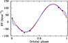 |
Fig. 6. Orbital NOT radial velocities (black points) with the simple Keplerian (red line) and the PHOEBE (blue line) fits that also include the predicted Rossiter-McLaughlin signature (Rossiter 1924; McLaughlin 1924). The uncertainties on the measurements are about the size of the plot symbols. |
Finally, the individual spectra were corrected for RV shifts, were coadded and compared to model spectra of different temperatures and surface gravities. The best fit was found for Teff = 7750 K, log g = 4.0, v sin i = 90 km s−1 (hence the previous choice of template). The primary star appears to be somewhat underabundant in heavy elements compared to the Sun ([M/H]= − 0.3 ± 0.2). Our spectra are insufficient to determine whether this is a true underabundance or if the primary star has some mild chemical peculiarity of the λ Bootis type, however.
3. System parameters
3.1. Data availability
The Gaia DR3 catalog (Gaia Collaboration 2016, 2023) gives a G magnitude of 11.82 and (BP − RP) = 0.34, which correspond to the mean values out of eclipse. The Gaia DR3 parallax of the system is 0.977 ± 0.019 mas. The reddening maps of Green et al. (2019) imply E(g − r) = 0.025 ± 0.015, consistent with Schlegel et al. (1998) (Ag = 0.139), which was taken as an upper limit to the interstellar reddening of the system given its Galactic latitude of +15 deg.
With the reddening relations by Zhang & Yuan (2023) and the transformations from the Gaia photometric system given in Table 5.9 of the Gaia DR3 release notes, we derived E(BP − RP) = 0.030 ± 0.018 and V = 11.86. The standard relations by Pecaut & Mamajek (2013) then suggest Teff = 7670 K, which agrees very well with the spectroscopic estimate above. With a bolometric correction of BC = +0.015, Av = 0.08 and the Gaia parallax Mbol = +1.74 ± 0.07 were derived (the error budget is dominated by the uncertainties in interstellar extinction and the V magnitude). With the bolometric magnitude of the Sun (Torres 2010), Mbol, ⊙ = 4.74, a mean out-of-eclipse system luminosity of L = 15.8 ± 1.1 L⊙ results.
Archival spectral flux measurements from 0.15 to 11.6 microns were collected. These data were taken from VizieR SED1 (Ochsenbein et al. 2000), which uses a systematic sky coverage of surveys such as Panoramic Survey Telescope And Rapid Response System (Pan-STARRS) (Chambers et al. 2016), Sloan Digital Sky Survey (SDSS) (Gunn et al. 1998), Two Micron All-Sky Survey (2MASS) (Skrutskie et al. 2006), Wide-field Infrared Survey Explorer (WISE) (Wright et al. 2010), and Galaxy Evolution Explorer (GALEX) (Bianchi et al. 2017). For EL CMi, we found 26 spectral points that we were able to use.
3.2. General approach
In what follows, the EL CMi system parameters are derived using two different approaches. In the first approach, the PHOEBE2 software is used to analyze the eclipsing light curve obtained with TESS plus the RV data from the primary star. In the second approach, our own code for fitting the spectral energy distribution (SED) coupled with a relatively simple eclipsing light-curve emulator is used to jointly analyze the TESS light curve, the available SED data, and the radial velocities for this source. Each approach is detailed in the following subsections.
3.3. PHOEBE analysis
The new-generation Wilson-Devinney code PHOEBE2 (Prša et al. 2016) was used to analyze the TESS eclipsing light curve of EL CMi and to simultaneously take into account the measured RV data points of the primary star. A Monte Carlo Markov chain (MCMC; Foreman-Mackey et al. 2013) wrapper was used to evaluate the uncertainties in the fitted parameters by sampling over a broad range of uninformed priors on the ratio of effective temperatures, primary radius, primary mass, mass ratio, secondary radius, orbital inclination, and systemic velocity.
The fitted light curve is shown in Fig. 7. The best-fitting parameters that result from this fit are shown in the first results column of Table 4. We simply fixed the Teff of the primary at 7750 K, as deduced from the spectroscopy (see Sect. 2.2). Both stars were modeled with Castelli et al. (2003) model atmospheres, where these atmospheres were used to derive the emergent intensity of each stellar surface element as well as the limb darkening via the PHOEBE2 interpolated limb-darkening scheme, and with a default gravity brightening (β = 0.32) and bolometric albedos (α = 0.6).
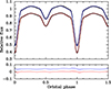 |
Fig. 7. Upper panel: Fit to the phase-binned TESS PDC light curve from Sector 34 (black points) compared to the fit derived with PHOEBE2 (blue line) and the combined SED + light-curve fitting approach (red line, data and fit shifted by 10% in intensity for clarity). Lower panel: Residuals from these fits. Blue: PHOEBE2, and red: SED + light-curve fitting, shifted by 4% in intensity for clarity. |
Binary parameters of TIC 321254859 (EL CMi) with two different methods.
The mass and Teff of the pulsating δ Scuti star are typical for these pulsators. On the other hand, the secondary, with a mass of only 0.93 M⊙ and radius of nearly 2 R⊙, strongly indicates a star that has lost its envelope during a prior episode of mass transfer. This is discussed further in the next section.
3.4. Light curve plus SED analysis
The SED of a binary can yield important information on the two stellar radii and the two Teff values when the distance to the source is known accurately. The SED by itself is not generally sufficient to yield all four of these parameters, however. Additionally, the eclipsing light curve contains key information on quantities such as the ratio of the two Teff values and the ratios of the stellar radii to the semi-major axis. The latter requires the system mass in order to translate R1/a and R2/a into information about the physical stellar radii, however. In turn, radial velocities can provide information about the masses. In any case, supplemental information about the radii and effective temperatures can indeed facilitate the inference of a number of the stellar properties from the SED data.
Under the assumption that the two stars in the binary have evolved coevally (i.e., without a prior episode of mass transfer), the SED can be fit with just four basic parameters: M1, M2, system age, and an interstellar extinction, AV. If the metallicity is not known from the spectral observations, it can be added as a fifth parameter.
The mass and age yield the radius and Teff of the two stars via stellar evolution tracks, and the SED can then be fit, provided that there is some other supplemental information such as the ratios of radii or Teff from a light-curve analysis, for instance, from PHOEBE2. Since PHOEBE2 does not have a built-in SED fitter, the light-curve fitting with PHOEBE2 and the SED fitting could be iterated with separate codes. We instead chose to write a combined SED fitter with a simplified light-curve emulator that can be used to jointly fit for both the SED and the eclipsing light curve. The code follows the description by Jayaraman et al. (2024). Briefly, the simplified light-curve emulator uses (i) spherical stars with limb darkening, and (ii) sets of sines and cosines to represent the out-of-eclipse behavior, including ellipsoidal light variations, illumination effects, and Doppler boosting (see, e.g. Carter et al. 2011).
The SED portion of the fitting code uses the MESA Isochrones and Stellar Tracks (MIST) evolution tracks (Choi et al. 2016; Dotter 2016; Paxton et al. 2011, 2015, 2019). For any given mass, age, and metallicity, the tracks provide the stellar radius and Teff. The stellar atmosphere models were taken from Castelli et al. (2003). The SED fitting portion of the code has been extensively tested on a number of multistellar systems, including binaries (Jayaraman et al. 2022b), triples (Rappaport et al. 2022), and even a sextuple star system (Powell et al. 2021). For EL CMi, metallicities of [Fe/H] = 0.0 and –0.3 were tested in keeping with what was learned from the stellar spectra (see Sect. 2.2). There was not much difference in the results depending on the metallicity.
This code was used to jointly fit the light curve, SED, and RV data for EL CMi, in agreement with the PHOEBE2 result. We found no viable solutions in which the two stars evolve in a coeval manner. Thus, there must have been a prior episode of mass transfer onto the current primary star (the pulsator). We therefore changed the fitted parameters to the following six quantities: primary and secondary mass (M1 and M2), radius and Teff of the secondary star (R2 and Teff, 2), the age of the primary star (since its rejuvenating accretion episode, τ), and AV.
The fitted light curve is shown in Fig. 7. Figure 8 shows a comparison of the observed to theoretical SED derived above as well as the fitted light curve. The agreement is satisfactory. Only the point in the far ultraviolet is somewhat off. This may be due to the wide bandwidth of the GALEX FUV filter and the steep continuum slope in this wavelength range, however (see Jayaraman et al. 2024).
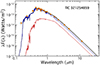 |
Fig. 8. Fit to the SED of the EL CMi system. The orange dots with the error bars show the observational values. The blue line is the SED of the primary star, the red line shows the SED of the secondary, and the black line shows the sum of the two. |
The parameters of the binary system are given in two columns of Table 4 along with some other derived parameters in Table 5. The second column of the results parameters in Table 4 lists the case without prior restrictions on the radius of the secondary star, except that it cannot overfill its Roche lobe. The third results column in Table 4 lists the restricted case when the secondary star always just fills its Roche lobe. This is motivated by evolutionary studies (see Sect. 4), which indicated that after the episode of rapid mass transfer, the donor star remains close to filling its Roche lobe for 1.3 Myr after the bulk of the mass transfer has ceased.
Other parameters of EL CMi from simultaneous light-curve and SED fitting.
A comparison of the three results columns in Table 4 paints a consistent picture of the stellar parameters for EL CMi. The main difference in the three results columns arises in the radii, depending on whether the secondary is assumed to fill its Roche lobe. In the former case, the primary is 24%±11% larger than the secondary, while in the latter case, the two stars are more nearly equal in size, with the secondary being slightly larger.
4. System evolution
As the data analysis suggests that the radius of the secondary is too large to be explained as a product of a single-star evolution, it is logical to suspect that EL CMi is a product of a system that has passed through a mass-transfer phase. To model the system as the result of a prior episode of mass transfer, we used the MESA code (Modules for Experiments in Stellar Astrophysics, Paxton et al. 2011, 2013, 2015, 2018, 2019; Jermyn et al. 2023, version 23.05.1) with the MESA-BINARY module under the assumption of an implicit mass-transfer rate.
To find a model that fits the parameters of the system, in particular the masses, radii, effective temperatures, and the orbital period, we built a grid of binary evolution tracks for initial periods spanning a range from 0.6 to 10 d and for initial masses in the range of 1.0–3.0 M⊙, with a constant step size of 0.2 d and 0.2 M⊙ respectively. Additionally, we used the results from Section 3 and we imposed the constraints that the initial total mass of the system should not be lower than 3.0 M⊙, but no higher than 3.5 M⊙ to account for some small mass loss. After obtaining an initial fit, we refined the grid resolution around the best-matching model by reducing the steps to 0.02 M⊙ in mass and 0.05 d in orbital period.
Four different values of metallicity, Z = 0.005, 0.010, 0.014, and 0.020, corresponding to [M/H] = −0.47, −0.16, −6.5 × 10⁻³, and 0.16, respectively, were used and scaled using the linear scaling relations by Choi et al. (2016) to determine the initial abundances of hydrogen and helium. We used the AGSS09 (Asplund et al. 2009) initial chemical composition of the stellar matter and the OPAL opacity tables supplemented with data from Ferguson et al. (2005) for lower temperatures. We treated convective instability using the Ledoux criterion, combined with the mixing length theory based on the model by Henyey et al. (1965). In regions that are stable according to the Ledoux criterion but unstable by the Schwarzschild criterion, we used semiconvective mixing with a scaling factor of αsc = 0.1, following the formalism of Langer et al. (1985). To mix regions in which the mean molecular weight was inverted, such as those that formed during mass accretion, we applied thermohaline mixing using the formalism of Kippenhahn et al. (1980) with an αth = 1 coefficient. As these models include neither rotation nor rotationally induced mixing, we used a minimum diffusive mixing coefficient of D = 10 cm2 s−1, which also allowed us to smooth out numerical noise or discontinuities in internal profiles.
The values of free stellar structure parameters were fixed according to the following theoretical models and asteroseismic calibrations. Given the primary mass, the convective-core overshooting parameter was set to fov = 0.02 for both components, in agreement with the values predicted by Claret & Torres (2016). Furthermore, the mixing length parameter and the fraction of mass lost from the system during mass transfer were set to αMLT = 1.5 and β = 0.2, in agreement with asteroseismic determinations for δ Scuti stars in post-mass-transfer binaries (e.g. Miszuda et al. 2022).
From each set of binary evolutionary tracks, we selected models that agreed with the measured current-epoch orbital period, and we calculated a normalized χ2 discriminant using observed and model masses, radii, and effective temperatures for these models. This resulted in a set of 40 models that fit the observations within 1σ and cluster around Porb, 0 ∈ (1.0, 1.05) d, Mdon, 0 ∈ (1.9, 2.06) M⊙ and Macc, 0 ∈ (0.9, 1.0) M⊙ for metallicities Z = 0.014 and Z = 0.02. A visualization of the best-fitting model is presented in Figure 9.
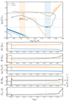 |
Fig. 9. Hertzsprung-Russel diagram and time evolution of the stellar masses, radii, effective temperatures, Roche-lobe filling factor, and the orbital period for the binary evolution track that best reproduces the observed parameters of the system. This track was computed for an initial orbital period Porb, 0 = 1.05 d, primary and secondary masses Mdon, 0 = 1.94 M⊙ and Macc, 0 = 0.94 M⊙, metallicity Z = 0.014, overshooting parameter fov = 0.02, mixing-length parameter αMLT = 1.5, and mass-transfer efficiency β = 0.2. The evolutionary tracks of the accretor and the donor are shown with orange and blue lines, respectively, and the same colors are used to indicate the observed ranges of the corresponding parameters, which are marked with shaded bands in the plots. The model at the time corresponding to the observed orbital period is marked with vertical dashed lines in the lower panels and with circular markers in the HR diagram. |
According to these models, the system is approximately 1.7 ± 0.3 Gyr old and is still undergoing mass transfer. The mass-transfer rate is currently fairly low at Ṁ ≈ 10−10 M⊙ yr−1. The fastest phase of mass transfer began when the system was ≈1 Gyr old, and it peaked at Ṁ ≈ 10−6 M⊙ yr−1. At this time, the donor star was in the later part of its main-sequence evolution, with a central hydrogen abundance of Xc = 0.26, while the accretor had barely evolved from the zero-age main sequence. This suggests that the binary went through type A mass transfer (MT) (Kippenhahn & Weigert 1967). Currently, after rejuvenation of the accretor and mass-ratio reversal, the donor is close to exhausting its central hydrogen (Xc < 0.1) and has retained a sufficiently thick hydrogen envelope to start ascending the red giant branch soon. On the other hand, the accretor is currently evolving through the main sequence, with a central hydrogen abundance of Xc = 0.45. These parameters are summarized in Table 6.
Summary of the key evolutionary parameters of the binary model.
Despite the decline in the mass-transfer rate following the initially faster phase, the donor remains close to Roche-lobe filling over an extended timescale, with Rdon/RRL ≲ 1. Although the donor is initially driven out of thermal equilibrium, it quickly recovers equilibrium after the mass ratio reverses. From this point onward, the donor becomes the less massive star, and its radius evolution, governed by hydrogen burning, begins to regulate the mass-transfer rate. As a result, the subsequent mass transfer proceeds on the nuclear timescale of the donor, allowing the stable low-rate Roche-lobe overflow configuration to persist until the central hydrogen is exhausted. During this phase, the donor maintains sufficient pressure support to avoid contraction, and the system evolves stably under slow mass exchange (e.g., Kolb & Ritter 1990).
Initially, the accretor temporarily departs from thermal equilibrium due to the rapid accretion. This results in an increased luminosity. The accretor regains equilibrium shortly after, however, and continues its main-sequence evolution with a steadily growing mass and radius. When it reaches the end of the mass-transfer phase, the accretor will attain a mass of 2.16 M⊙, cross the Hertzsprung gap, and become a red giant.
As mass transfer continues, the donor gradually loses its hydrogen-rich envelope. When the mass transfer ceases, the envelope is no longer massive enough (M = 0.2 M⊙) to maintain efficient shell hydrogen burning or to provide the pressure required to compress the core toward helium ignition. At this point, the central temperature only reaches log Tc ≈ 7.52, and the helium core mass is limited to Mcore ≈ 0.17 M⊙. These values are both well below the thresholds required for helium ignition. Consequently, instead of ascending the RGB up to helium ignition, the star will evolve toward the pre-helium white dwarf (pre-He WD) phase. Despite its relatively high initial mass, the donor ultimately avoids helium ignition and becomes a low-mass helium white dwarf star.
At an age of ≈2.9 Gyr, the accretor star evolves into an AGB star and starts mass transfer to the helium white dwarf. At this point, the AGB star has a helium core mass of 0.488 M⊙ and a carbon/oxygen core of 0.280 M⊙. Since the binary mass ratio is high, the mass transfer is dynamically unstable, and the binary system will enter a common envelope (CE) phase. By comparing the binding energy of the envelope with the orbital energy of the system, we find that the CE cannot be ejected even for a CE ejection efficiency of 1.0. Consequently, the binary system ultimately merges into a single star.
It is unclear whether the ongoing accretion in the current evolutionary state of the system affects the triaxial pulsations of the primary (the accretor), but we do not expect strong effects. Because the primary is underfilling its Roche lobe and its current accretion rate is low, we do not expect substantial deviations from the hydrostatic equilibrium that is assumed in the triaxial pulsation model. The accretion power is Lac ≈ GMṀ/R ≈ 0.003 L⊙ (Ṁ/10−10 M⊙/yr), which is much lower than the luminosity of the primary. Its structure and pulsations are therefore unlikely to be greatly modified.
5. Discussion and conclusions
The first objects called “tidally tilted pulsators” were explained as stars whose pulsational axis was pulled into the orbital plane and pointed at their close companion star at each point in the orbit. The first such pulsator, HD 74423, had a single dipole oscillation mode whose amplitude was also enhanced in one hemisphere. This motivated the term “single-sided pulsator” (Handler et al. 2020). The second such object, CO Cam, showed multiperiodic axisymmetric pulsations with a higher amplitude in the direction of the companion (Kurtz et al. 2020), and the third object, TIC 63328020, appeared to be distinctly different with its tesseral tidally tilted dipole mode (Rappaport et al. 2021).
The idea that stars can pulsate triaxially was based on the observational studies of TIC 184743498 by Zhang et al. (2024) and of TIC 435850195 by Jayaraman et al. (2024), which demonstrated that both objects have very many tidally tilted dipole modes. The geometries of these binary systems, and hence the inclination of the tilted stellar pulsational axis to the line of sight, however, made an explanation of these objects in terms of simple tidally tilted pulsators impossible because the observed amplitude and phase modulations of the individual pulsations during the orbit are predictable depending on the type of the pulsation modes and on the orbital geometry of the system (Reed et al. 2005). The behavior of the pulsations of these latter two stars did not conform to a simple picture of tidal tilting, but could be explained with pulsation around three different axes.
The theoretical foundation for this interpretation was provided by Fuller et al. (2025), who showed that the different azimuthal orders of a dipole frequency multiplet are tidally coupled in these systems. Thus, they align with the three principal axes of the triaxially deformed pulsating star. Based on this theory, theoretical predictions of the manifestations of nonradial quadrupole oscillation modes were provided. We presented the first observational detection of such a quadrupole mode.
The primary component of EL CMi is the third object in which pulsation modes that only occur in triaxially distorted stars reported. It is therefore logical to suspect that the previously discovered tidally tilted or single-sided pulsators may be just special cases of triaxial pulsators. After all, all of these objects are distorted into triaxial shapes, and their pulsation modes conform to the same framework. The single mode of HD 74423 is consistent with a tidally enhanced Y10x mode, whereas the four modes of CO Cam appear to be of the same type. The behavior of the single mode of TIC 63328020, which was originally classified as a tidally tilted l = 1, m = 1 (Y11x) mode, is also consistent with a Y10y mode. The numerous mode doublets and one triplet in TZ Dra (Kahraman Aliçavuş et al. 2022) are also consistent with Y10x and Y10y modes, respectively, and the pulsation modes of the subdwarf B star HD 265435 (Jayaraman et al. 2022a) conform to the predictions of the behavior of modes in triaxially distorted stars by Fuller et al. (2025) as well.
The evolutionary state of the tidally tilted or triaxial pulsators with a main-sequence star as the primary components show for EL CMi, TIC 63328020 and TZ Dra that they have undergone or are undergoing mass transfer, whereas HD 74423, CO Cam, TIC 184743498, and TIC 435850195 are detached systems. The appearance of these special types of pulsation therefore appears to be not connected to a particular evolutionary phase of close binary systems.
The pulsating star in EL CMi is a very simple and clear example that demonstrates that the main features of the theoretical description of Fuller modes are consistent with observations. It is reasonable to expect that stars with richer, more complicated pulsation spectra will be discovered in the future. These pulsations in essence come with an observational identification of the underlying modes and occur in stars that can be characterized with a high degree of confidence and accuracy because they are located in binary and multiple systems. These objects might therefore be used for detailed asteroseismic studies based on oscillations that occur around three different symmetry axes. In other words, these objects hold the promise of enabling us to study the interior structure of distant stars in three dimensions.
Data availability
We make all files needed to recreate our MESA-BINARY results publicly available at Zenodo: https://zenodo.org/records/15745684
Acknowledgments
GH and AM both thank the Polish National Center for Science (NCN) for supporting this study through grant 2021/43/B/ST9/02972 and Filiz Kahraman Aliçavuş for her comments on the spectrum of the target. DJ acknowledges support from the Agencia Estatal de Investigación del Ministerio de Ciencia, Innovación y Universidades (MCIU/AEI) under grant “Nebulosas planetarias como clave para comprender la evolución de estrellas binarias” and the European Regional Development Fund (ERDF) with reference PID-2022-136653NA-I00 (DOI: 10.13039/501100011033). DJ also acknowledges support from the Agencia Estatal de Investigación del Ministerio de Ciencia, Innovación y Universidades (MCIU/AEI) under grant “Revolucionando el conocimiento de la evolución de estrellas poco masivas” and the European Union Next Generation EU/PRTR with reference CNS2023-143910 (DOI: 10.13039/501100011033). H-LC is supported by the National Key R&D Program of China (grant Nos. 2021YFA1600403), the National Natural Science Foundation of China (grant Nos. 12288102, 12333008 and 12422305). VK acknowledges support from NSF grant AST-2206814. This paper includes data collected by the TESS mission. Funding for the TESS mission is provided by the NASA Science Mission Directorate. The QLP data used in this work were obtained from MAST (https://dx.doi.org/10.17909/t9-r086-e880), hosted by the Space Telescope Science Institute (STScI). STScI is operated by the Association of Universities for Research in Astronomy, Inc., under NASA contract NAS 5–26555. This work also presents results from the European Space Agency (ESA) space mission Gaia. Gaia data are being processed by the Gaia Data Processing and Analysis Consortium (DPAC). Funding for the DPAC is provided by national institutions, in particular the institutions participating in the Gaia MultiLateral Agreement (MLA). The Gaia mission website is https://www.cosmos.esa.int/gaia. The Gaia archive website is https://archives.esac.esa.int/gaia. This research has also made use of the VizieR catalogue access tool, CDS, Strasbourg, France. Software: This paper made use of the following codes/packages: LIGHTKURVE (Lightkurve Collaboration 2018), IRAF (Tody 1986) SPECTRUM (Gray & Corbally 1994) PERIOD04 (Lenz & Breger 2005) MESA (Paxton et al. 2011, 2013, 2015, 2018, 2019; Jermyn et al. 2023).
References
- Aerts, C. 2021, Rev. Mod. Phys., 93, 015001 [Google Scholar]
- Asplund, M., Grevesse, N., Sauval, A. J., & Scott, P. 2009, ARA&A, 47, 481 [NASA ADS] [CrossRef] [Google Scholar]
- Baglin, A., Auvergne, M., Boisnard, L., et al. 2006, in 36th COSPAR Scientific Assembly, 36, 3749 [Google Scholar]
- Balona, L. A. 2014, MNRAS, 439, 3453 [NASA ADS] [CrossRef] [Google Scholar]
- Baran, A. S., & Koen, C. 2021, Acta Astron., 71, 113 [Google Scholar]
- Bedding, T. R., Murphy, S. J., Hey, D. R., et al. 2020, Nature, 581, 147 [NASA ADS] [CrossRef] [Google Scholar]
- Benz, W., Broeg, C., Fortier, A., et al. 2021, Exp. Astron., 51, 109 [Google Scholar]
- Bianchi, L., Shiao, B., & Thilker, D. 2017, ApJS, 230, 24 [Google Scholar]
- Bókon, A., Bíró, I. B., & Derekas, A. 2025, A&A, 693, A259 [NASA ADS] [CrossRef] [EDP Sciences] [Google Scholar]
- Bowman, D. M., Burssens, S., Pedersen, M. G., et al. 2019, Nat. Astron., 3, 760 [Google Scholar]
- Breger, M., Stich, J., Garrido, R., et al. 1993, A&A, 271, 482 [NASA ADS] [Google Scholar]
- Burssens, S., Bowman, D. M., Michielsen, M., et al. 2023, Nat. Astron., 7, 913 [NASA ADS] [CrossRef] [Google Scholar]
- Carter, J. A., Rappaport, S., & Fabrycky, D. 2011, ApJ, 728, 139 [NASA ADS] [CrossRef] [Google Scholar]
- Castelli, F., & Kurucz, R. L. 2003, in Modelling of Stellar Atmospheres, eds. N. Piskunov, W. W. Weiss, & D. F. Gray, IAU Symposium, 210, A20 [Google Scholar]
- Chambers, K. C., Magnier, E. A., Metcalfe, N., et al. 2016, arXiv e-prints [arXiv:1612.05560] [Google Scholar]
- Choi, J., Dotter, A., Conroy, C., et al. 2016, ApJ, 823, 102 [Google Scholar]
- Claret, A., & Torres, G. 2016, A&A, 592, A15 [NASA ADS] [CrossRef] [EDP Sciences] [Google Scholar]
- Dotter, A. 2016, ApJS, 222, 8 [Google Scholar]
- Ferguson, J. W., Alexander, D. R., Allard, F., et al. 2005, ApJ, 623, 585 [Google Scholar]
- Foreman-Mackey, D., Hogg, D. W., Lang, D., & Goodman, J. 2013, PASP, 125, 306 [Google Scholar]
- Fuller, J., Kurtz, D. W., Handler, G., & Rappaport, S. 2020, MNRAS, 498, 5730 [NASA ADS] [CrossRef] [Google Scholar]
- Fuller, J., Rappaport, S., Jayaraman, R., Kurtz, D., & Handler, G. 2025, ApJ, 979, 80 [Google Scholar]
- Gaia Collaboration (Prusti, T., et al.) 2016, A&A, 595, A1 [NASA ADS] [CrossRef] [EDP Sciences] [Google Scholar]
- Gaia Collaboration (Vallenari, A., et al.) 2023, A&A, 674, A1 [NASA ADS] [CrossRef] [EDP Sciences] [Google Scholar]
- Gilliland, R. L., Brown, T. M., Christensen-Dalsgaard, J., et al. 2010, PASP, 122, 131 [Google Scholar]
- Gootkin, K., Hon, M., Huber, D., et al. 2024, ApJ, 972, 137 [Google Scholar]
- Gray, R. O., & Corbally, C. J. 1994, AJ, 107, 742 [Google Scholar]
- Green, G. M., Schlafly, E., Zucker, C., Speagle, J. S., & Finkbeiner, D. 2019, ApJ, 887, 93 [NASA ADS] [CrossRef] [Google Scholar]
- Gunn, J. E., Carr, M., Rockosi, C., et al. 1998, AJ, 116, 3040 [NASA ADS] [CrossRef] [Google Scholar]
- Handler, G., Kurtz, D. W., Rappaport, S. A., et al. 2020, Nat. Astron., 4, 684 [Google Scholar]
- Henyey, L., Vardya, M. S., & Bodenheimer, P. 1965, ApJ, 142, 841 [Google Scholar]
- Hon, M., Huber, D., Kuszlewicz, J. S., et al. 2021, ApJ, 919, 131 [NASA ADS] [CrossRef] [Google Scholar]
- Huber, D., Chaplin, W. J., Christensen-Dalsgaard, J., et al. 2013, ApJ, 767, 127 [Google Scholar]
- Jayaraman, R., Handler, G., Rappaport, S. A., et al. 2022a, ApJ, 928, L14 [NASA ADS] [CrossRef] [Google Scholar]
- Jayaraman, R., Rappaport, S. A., Nelson, L., et al. 2022b, ApJ, 936, 123 [Google Scholar]
- Jayaraman, R., Rappaport, S. A., Powell, B., et al. 2024, ApJ, 975, 121 [Google Scholar]
- Jennings, Z., Southworth, J., Rappaport, S. A., et al. 2024, MNRAS, 533, 2705 [Google Scholar]
- Jermyn, A. S., Bauer, E. B., Schwab, J., et al. 2023, ApJS, 265, 15 [NASA ADS] [CrossRef] [Google Scholar]
- Kahraman Aliçavuş, F., Handler, G., Aliçavuş, F., et al. 2022, MNRAS, 510, 1413 [Google Scholar]
- Kippenhahn, R., & Weigert, A. 1967, Z. Astrophys., 65, 251 [NASA ADS] [Google Scholar]
- Kippenhahn, R., Ruschenplatt, G., & Thomas, H. C. 1980, A&A, 91, 175 [Google Scholar]
- Koch, D. G., Borucki, W. J., Basri, G., et al. 2010, ApJ, 713, L79 [Google Scholar]
- Kolb, U., & Ritter, H. 1990, A&A, 236, 385 [NASA ADS] [Google Scholar]
- Kostov, V. B., Powell, B. P., Fornear, A. U., et al. 2025, ApJS, 279, 50 [Google Scholar]
- Kurtz, D. W. 2022, ARA&A, 60, 31 [NASA ADS] [CrossRef] [Google Scholar]
- Kurtz, D. W., Handler, G., Rappaport, S. A., et al. 2020, MNRAS, 494, 5118 [Google Scholar]
- Kurtz, D. W., Handler, G., Holdsworth, D. L., et al. 2025, MNRAS, 536, 2103 [Google Scholar]
- Langer, N., El Eid, M. F., & Fricke, K. J. 1985, A&A, 145, 179 [NASA ADS] [Google Scholar]
- Lenz, P., & Breger, M. 2005, CoAst, 146, 53 [NASA ADS] [Google Scholar]
- Lightkurve Collaboration (Cardoso, J. V. d. M., et al.) 2018, Astrophysics Source Code Library [record ascl:1812.013] [Google Scholar]
- McLaughlin, D. B. 1924, ApJ, 60, 22 [Google Scholar]
- Miszuda, A., Kołaczek-Szymański, P. A., Szewczuk, W., & Daszyńska-Daszkiewicz, J. 2022, MNRAS, 514, 622 [NASA ADS] [CrossRef] [Google Scholar]
- Morris, R. L., Twicken, J. D., Smith, J. C., et al. 2020, in Kepler Data Processing Handbook: Photometric Analysis, Kepler Science Document KSCI-19081-003, ed. J. M. Jenkins, 6 [Google Scholar]
- Ochsenbein, F., Bauer, P., & Marcout, J. 2000, A&AS, 143, 23 [NASA ADS] [CrossRef] [EDP Sciences] [Google Scholar]
- Paxton, B., Bildsten, L., Dotter, A., et al. 2011, ApJS, 192, 3 [Google Scholar]
- Paxton, B., Cantiello, M., Arras, P., et al. 2013, ApJS, 208, 4 [Google Scholar]
- Paxton, B., Marchant, P., Schwab, J., et al. 2015, ApJS, 220, 15 [Google Scholar]
- Paxton, B., Schwab, J., Bauer, E. B., et al. 2018, ApJS, 234, 34 [NASA ADS] [CrossRef] [Google Scholar]
- Paxton, B., Smolec, R., Schwab, J., et al. 2019, ApJS, 243, 10 [Google Scholar]
- Pecaut, M. J., & Mamajek, E. E. 2013, ApJS, 208, 9 [Google Scholar]
- Powell, B. P., Kostov, V. B., Rappaport, S. A., et al. 2021, AJ, 161, 162 [NASA ADS] [CrossRef] [Google Scholar]
- Prochaska, J. X., Hennawi, J. F., Westfall, K. B., et al. 2020a, J. Open Source Softw., 5, 2308 [NASA ADS] [CrossRef] [Google Scholar]
- Prochaska, J. X., Hennawi, J., Cooke, R., et al. 2020b, https://doi.org/10.5281/zenodo.3743493 [Google Scholar]
- Prša, A., Conroy, K. E., Horvat, M., et al. 2016, ApJS, 227, 29 [Google Scholar]
- Rappaport, S. A., Kurtz, D. W., Handler, G., et al. 2021, MNRAS, 503, 254 [NASA ADS] [Google Scholar]
- Rappaport, S. A., Borkovits, T., Gagliano, R., et al. 2022, MNRAS, 513, 4341 [NASA ADS] [CrossRef] [Google Scholar]
- Rauer, H., Catala, C., Aerts, C., et al. 2014, Exp. Astron., 38, 249 [Google Scholar]
- Reed, M. D., Brondel, B. J., & Kawaler, S. D. 2005, ApJ, 634, 602 [NASA ADS] [CrossRef] [Google Scholar]
- Ricker, G. R., Winn, J. N., Vanderspek, R., et al. 2015, J. Astron. Telesc. Instrum. Syst., 1, 014003 [Google Scholar]
- Rossiter, R. A. 1924, ApJ, 60, 15 [Google Scholar]
- Schlegel, D. J., Finkbeiner, D. P., & Davis, M. 1998, ApJ, 500, 525 [Google Scholar]
- Skrutskie, M. F., Cutri, R. M., Stiening, R., et al. 2006, AJ, 131, 1163 [NASA ADS] [CrossRef] [Google Scholar]
- Smith, J. C., Stumpe, M. C., Van Cleve, J. E., et al. 2012, PASP, 124, 1000 [Google Scholar]
- Stumpe, M. C., Smith, J. C., Van Cleve, J. E., et al. 2012, PASP, 124, 985 [Google Scholar]
- Tody, D. 1986, in Instrumentation in Astronomy VI, ed. D. L. Crawford, Society of Photo-Optical Instrumentation Engineers (SPIE) Conference Series, 627, 733 [NASA ADS] [CrossRef] [Google Scholar]
- Torres, G. 2010, AJ, 140, 1158 [Google Scholar]
- Twicken, J. D., Clarke, B. D., Bryson, S. T., et al. 2010, in Software and Cyberinfrastructure for Astronomy, eds. N. M. Radziwill, & A. Bridger, Society of Photo-Optical Instrumentation Engineers (SPIE) Conference Series, 7740, 774023 [Google Scholar]
- Van Reeth, T., Johnston, C., Southworth, J., et al. 2023, A&A, 671, A121 [NASA ADS] [CrossRef] [EDP Sciences] [Google Scholar]
- Wright, E. L., Eisenhardt, P. R. M., Mainzer, A. K., et al. 2010, AJ, 140, 1868 [Google Scholar]
- Zhang, R., & Yuan, H. 2023, ApJS, 264, 14 [NASA ADS] [CrossRef] [Google Scholar]
- Zhang, V., Rappaport, S., Jayaraman, R., et al. 2024, MNRAS, 528, 3378 [Google Scholar]
A.-C. Simon & T. Boch: http://vizier.cds.unistra.fr/vizier/sed/
All Tables
All Figures
|
Fig. 1. Phase-folded TESS Sector 34 PDCSAP light curve of EL CMi without the pulsation. |
| In the text | |
|
Fig. 2. Échelle diagram for EL CMi from Sectors 34 (black), 61 (red), and 88 (blue). Top: All data. Bottom: Primary eclipses removed from the light curve. The sizes of the plot symbols relate to the logarithm of the pulsation amplitude; the cross marks the expected location of the centroid of mode ν2. |
| In the text | |
|
Fig. 3. Fourier transforms of the Sector 34 TESS data for EL CMi with subsequent pre-whitening steps (first, only the orbital harmonics, then the orbital harmonics plus 7, 18, and 19 pulsation frequencies indicated by the blue arrows, respectively). The inset in the top panel shows the spectral window function of this dataset. The level of the S/N curve is applicable for all of these amplitude spectra, but is plotted only once for clarity. |
| In the text | |
|
Fig. 4. Same as Fig. 3, but for the data without the primary eclipses. The inset in the top panel shows the spectral window function of this dataset. |
| In the text | |
|
Fig. 5. Run of the pulsation amplitude and phase for the three main modes of EL CMi. Black: Sector 34 data. Red: Sector 61 data. Blue: Sector 88 data. Upper panel: Orbital light curve. Second and third panels: All data. Lower two panels: Reconstructions from the data without the primary eclipses. The frequencies are for the multiplet centroids. |
| In the text | |
|
Fig. 6. Orbital NOT radial velocities (black points) with the simple Keplerian (red line) and the PHOEBE (blue line) fits that also include the predicted Rossiter-McLaughlin signature (Rossiter 1924; McLaughlin 1924). The uncertainties on the measurements are about the size of the plot symbols. |
| In the text | |
|
Fig. 7. Upper panel: Fit to the phase-binned TESS PDC light curve from Sector 34 (black points) compared to the fit derived with PHOEBE2 (blue line) and the combined SED + light-curve fitting approach (red line, data and fit shifted by 10% in intensity for clarity). Lower panel: Residuals from these fits. Blue: PHOEBE2, and red: SED + light-curve fitting, shifted by 4% in intensity for clarity. |
| In the text | |
|
Fig. 8. Fit to the SED of the EL CMi system. The orange dots with the error bars show the observational values. The blue line is the SED of the primary star, the red line shows the SED of the secondary, and the black line shows the sum of the two. |
| In the text | |
|
Fig. 9. Hertzsprung-Russel diagram and time evolution of the stellar masses, radii, effective temperatures, Roche-lobe filling factor, and the orbital period for the binary evolution track that best reproduces the observed parameters of the system. This track was computed for an initial orbital period Porb, 0 = 1.05 d, primary and secondary masses Mdon, 0 = 1.94 M⊙ and Macc, 0 = 0.94 M⊙, metallicity Z = 0.014, overshooting parameter fov = 0.02, mixing-length parameter αMLT = 1.5, and mass-transfer efficiency β = 0.2. The evolutionary tracks of the accretor and the donor are shown with orange and blue lines, respectively, and the same colors are used to indicate the observed ranges of the corresponding parameters, which are marked with shaded bands in the plots. The model at the time corresponding to the observed orbital period is marked with vertical dashed lines in the lower panels and with circular markers in the HR diagram. |
| In the text | |
Current usage metrics show cumulative count of Article Views (full-text article views including HTML views, PDF and ePub downloads, according to the available data) and Abstracts Views on Vision4Press platform.
Data correspond to usage on the plateform after 2015. The current usage metrics is available 48-96 hours after online publication and is updated daily on week days.
Initial download of the metrics may take a while.