| Issue |
A&A
Volume 702, October 2025
|
|
|---|---|---|
| Article Number | A180 | |
| Number of page(s) | 10 | |
| Section | Galactic structure, stellar clusters and populations | |
| DOI | https://doi.org/10.1051/0004-6361/202556239 | |
| Published online | 17 October 2025 | |
The Small Magellanic Cloud through the lens of the James Webb Space Telescope: Binaries and the mass function in the galaxy’s outskirts
1
Dipartimento di Fisica e Astronomia “Galileo Galilei”, Univ. di Padova,
Vicolo dell’Osservatorio 3,
Padova
35122,
Italy
2
Istituto Nazionale di Astrofisica – Osservatorio Astronomico di Padova,
Vicolo dell’Osservatorio 5,
Padova
35122,
Italy
3
Research School of Astronomy and Astrophysics, Australian National University,
Canberra,
ACT 2611,
Australia
4
South-Western Institute for Astronomy Research, Yunnan University,
Kunming
650500,
PR China
★ Corresponding author: This email address is being protected from spambots. You need JavaScript enabled to view it.
Received:
3
July
2025
Accepted:
8
September
2025
Abstract
The stellar initial mass function (IMF) and the fraction of binary systems are fundamental ingredients that govern the formation and evolution of galaxies. Whether the IMF is universal or varies with environment remains one of the central open questions in astrophysics. Dwarf galaxies such as the Small Magellanic Cloud (SMC), with their low metallicity and diffuse star-forming regions, offer critical laboratories to address this issue. In this work, we exploit ultra-deep photometry from the James Webb Space Telescope to investigate the stellar populations in the field of the SMC. Using the mF322W2 versus mF115W – mF322W2 color-magnitude diagram (CMD), we derive the luminosity function and measure the fraction of unresolved binary systems. We find a binary fraction of fbinq>0.6 = 0.14 ± 0.01, consistent with results from synthetic CMDs incorporating the metallicity distribution of the SMC. Additionally, the measured binary fraction in the SMC field is consistent with those observed in Galactic open clusters and Milky Way field stars of similar ages and masses, suggesting similar binary formation and evolutionary processes across these low-density environments. By combining the luminosity function with the best-fit isochrone, we derive the mass function (MF) down to 0.22 M⊙, the lowest mass limit reached for the SMC to date. The resulting MF follows a power-law with a slope of α = −1.99 ± 0.08. This value is shallower than the canonical Salpeter slope of α = −2.35, providing new evidence for IMF variations in low-metallicity and low-density environments.
Key words: techniques: photometric / binaries: general / Hertzsprung-Russell and C-M diagrams / stars: luminosity function, mass function / stars: Population II / Magellanic Clouds
© The Authors 2025
 Open Access article, published by EDP Sciences, under the terms of the Creative Commons Attribution License (https://creativecommons.org/licenses/by/4.0), which permits unrestricted use, distribution, and reproduction in any medium, provided the original work is properly cited.
This article is published in open access under the Subscribe to Open model. This email address is being protected from spambots. You need JavaScript enabled to view it. to support open access publication.
1 Introduction
The Small Magellanic Cloud (SMC) provides a unique and valuable laboratory for studying stellar populations in a low-metallicity, extragalactic environment. Its proximity, low foreground extinction, and relatively low crowding compared to more massive galaxies enable us to resolve individual stars across a broad range of stellar masses, from low-mass main sequence (MS) stars to evolved giants. As a result, the SMC has become a cornerstone for testing stellar evolution models and investigating the processes that shape galaxies beyond the Milky Way (e.g., Dobbie et al. 2014a,b; Rubele et al. 2018; Mackey et al. 2018; Pastorelli et al. 2019). Among the fundamental ingredients that regulate star formation and evolution are the initial mass function (IMF) and the fraction of binaries, both of which influence the dynamical evolution of stellar systems, the rates of supernovae and chemical enrichment, and the production of exotic objects such as blue stragglers, X-ray binaries, and gravitational wave sources.
Despite their importance, both the IMF and the binary fraction remain poorly constrained in external galaxies, particularly in the field populations of low-mass systems like the SMC. While studies of young clusters in the Magellanic Clouds have provided valuable insights into the high-mass IMF and short-period massive binaries (e.g., Dunstall et al. 2015; Sabbi et al. 2016; Almeida et al. 2017; Schneider et al. 2018; Kalari et al. 2018), much less is known about the binary properties of field stars, especially at intermediate and low masses. In this regime, unresolved binaries can significantly bias luminosity and mass function (MF) estimates by mimicking brighter, higher-mass single stars in the color-magnitude diagram (CMD). Properly accounting for binary contamination is therefore crucial for deriving accurate stellar MFs.
The interplay between the IMF and binaries is especially relevant in the context of the ongoing debate about the universality of the IMF, that is, whether its shape remains constant across different environments and over cosmic time. While the classical Salpeter (1955) IMF describes a power-law distribution with slope α = −2.35 over 0.4 ≲ M/M⊙ ≲ 10, numerous studies have suggested deviations from this form. Simulations and observations from the Atacama Large Millimeter Array (ALMA) point to top-heavy IMFs in early stars and dense star-forming regions (e.g., Abel et al. 2002; Bromm et al. 2002; Pouteau et al. 2022), whereas integrated-light studies of giant ellipticals suggest bottom-heavy IMFs dominated by low-mass stars (van Dokkum & Conroy 2010; Conroy & van Dokkum 2012). Stellar kinematic analyses have reached similar conclusions (Cappellari et al. 2012).
Although integrated-light studies offer IMF constraints in diverse environments, they are inherently model-dependent. Conversely, resolved stellar populations enable more robust IMF measurements, free from many of these uncertainties (e.g., Luhman et al. 2009; Milone et al. 2012a; Sollima & Baumgardt 2017; Dondoglio et al. 2022; Cordoni et al. 2023; Baumgardt et al. 2023; Marino et al. 2024a). However, these studies are mostly confined to the Milky Way and its clusters, limiting the parameter space in which IMF variations can be tested.
Dwarf galaxies like the SMC and ultra-faint dwarfs (UFDs) offer ideal laboratories for probing IMF universality across a broader range of conditions. They differ significantly from the Milky Way in terms of morphology, metallicity, star formation history, and stellar density. Additionally, their extremely long two-body relaxation times (e.g., ~2 × 10⁴ Gyr in the SMC; Gennaro et al. 2018a) imply that dynamical effects are negligible, and, thus, that the primordial MF is preserved. Observations with the Hubble Space Telescope (HST) and the James Webb Space Telescope (JWST) have enabled direct star counts in these systems, revealing evidence of a shallower MF slope compared to the canonical value. For example, Wyse et al. (2002) found α = −1.8 in Ursa Minor, while Geha et al. (2013) and Gennaro et al. (2018a,b) report similarly shallow slopes in several UFDs.
In this context, Kalirai et al. (2013) used deep HST observations with the Wide Field Camera of the Advanced Camera for Surveys (WFC/ACS) to investigate the IMF in the outskirts of the SMC. They reported a best-fit IMF slope of  , which is shallower than the canonical Salpeter value. Moreover, their analysis demonstrated that the data are well represented by a single-component IMF.
WFC/ACS observations allowed Kalirai et al. (2013) to probe stellar masses down to ~0.4 M⊙. In our work, we leveraged the exceptional capabilities of JWST to measure the fraction of blue straggler stars (BSSs) and the binary fraction along the MS, and to investigate the stellar mass distribution in the SMC field down to ~0.2 M⊙. This study provides the first estimate of the photometric binary fraction in the SMC and represents the deepest exploration of the IMF in an extragalactic environment to date. By accounting for binary populations in our analysis, we aim to derive an accurate IMF and assess possible environmental deviations from the IMF observed in the Milky Way and nearby dwarf galaxies.
The paper is organized as follows. In Section 2, we describe the photometric dataset and the data reduction procedures. Section 3 presents the derivation of the binary fraction in the SMC field. In Section 4, we determine the MF and its slope. Finally, Section 5 summarizes our key findings and conclusions.
2 Observations and data reduction
To measure the binary fraction and investigate the low-mass end of the stellar MF in the field of the SMC, we used the photometric catalogs provided by Marino et al. (2024a), which are obtained from images in the F115W and F322W2 filters of the Near-InfraRed Camera (NIRCam) on board the JWST. These data were collected during the first JWST observing cycle as part of the GO-2560 program (PI: A.F. Marino). This program is designed to investigate multiple stellar populations among low-mass stars in the globular cluster (GC) NGC 104 (47 Tucanae), leveraging the synergy between the Near-InfraRed Spectrograph (NIRSpec) and NIRCam facilities (see Marino et al. 2024a,b, for details on the dataset and on the program). Although the primary target of these observations is 47 Tucanae, the specific field observed, located at α ~ 00h21m16s and δ ~ −72d06m16s, also encompasses a line of sight intersecting the outskirts of the SMC. In particular, the analyzed SMC populations are ~2.5° (2.7 kpc) west of the galaxy’s center.
The footprints of the data used in this study are shown in green in the inset of Fig. 1. For comparison, we also show in red the footprints of the observations employed by Kalirai et al. (2013) to measure the IMF in the SMC field in the mass range 0.37–0.93 M⊙. Although their field lies in close proximity to ours, it is centered at α ~ 00h22m39s and δ ~ −72d04m04s and covers a distinct region. This spatial separation enables us to provide an independent determination of the IMF in the SMC field.
The methods used to reduce the observations are described in detail in Marino et al. (2024a, see also Milone et al. 2023b). Briefly, the measurement of stellar fluxes and positions involved a two-step process. In the first step, photometry was performed using the program img2xym, originally developed by Anderson & King (2006) to reduce HST images. This program utilizes a spatially variable point spread function to determine stellar positions and magnitudes from each individual exposure. Magnitudes were standardized to a common photometric zero-point, using the deepest exposure as the reference frame, while geometric distortions were corrected with solutions provided by Milone et al. (2023b).
The second step involved refining photometry and astrometry using the KS2 program, an updated version of kitchen_sync by Anderson et al. (2008). KS2 incorporates specialized methods tailored to optimize photometry for stars of varying luminosities (see Sabbi et al. 2016; Bellini et al. 2017; Nardiello et al. 2018, for details). It also provides diagnostic parameters to assess photometric and astrometric quality. These parameters were used, following the approach of Milone et al. (2023a, see their Sect. 2.4), to select a reliable sample of well-measured stars.
The photometry was calibrated to the Vega system using the procedure described by Milone et al. (2023a) and zero-points available on the Space Telescope Science Institute’s web page1. Furthermore, reddening variations across the field of view were confirmed to be insignificant (Legnardi et al. 2023), so no corrections for differential reddening were necessary.
To assess the uncertainties and the completeness level of our photometry, we performed artificial star (AS) tests following the methodology outlined by Anderson et al. (2008). We generated a catalog of 105 ASs with fixed positions and fluxes, distributing them across the field of view to match the spatial distribution of the real stars. Their magnitudes were assigned based on the fiducial line of the SMC MS in the mF322W2 versus mF115W − mF322W2 CMD. The ASs were reduced using the KS2 program, following the same procedures applied to real stars. We used diagnostic parameters provided by KS2 to assess the quality of the recovered sources.
To quantify the completeness, we binned the ASs into magnitude intervals of 0.3 mag. In each bin, the completeness fraction was calculated as the ratio of recovered to injected stars. We determined that the 50% completeness limit is reached at mF322W2 = 26.22 mag.
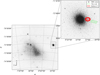 |
Fig. 1 Image of the SMC obtained from the Digitized Sky Survey 2. The inset provides a close-up view of the region near 47 Tucanae where the observations for this study were carried out. The NIRCam field of view analyzed in this work is outlined in green, and the footprints of the observations used by Kalirai et al. (2013) are shown in red. The white cross marks the position of the SMC center (Piatti 2021). North is up, and east is to the left. |
3 The color-magnitude diagram of the Small Magellanic Cloud
A visual inspection of the mF322W2 versus mF115W − mF322W2 CMD, shown in the left panel of Fig. 2, reveals the presence of two distinct stellar populations. The redder sequence (gray points) corresponds to the faint end of the 47 Tucanae MS, while the bluer sequence (black points) traces field stars belonging to the SMC. In addition, the gray points located in the bottom-left corner of the CMD likely represent the white dwarf cooling sequence of 47 Tucanae.
The right panel of Fig. 2 isolates the SMC field population, highlighting a significant broadening of the MS in the mF115W − mF322W2 color that exceeds expectations from photometric uncertainties alone, as indicated by the error bars on the left corner. This spread is primarily driven by variations in stellar metallicity. Numerous photometric and spectroscopic studies have confirmed the presence of a radial metallicity gradient within the SMC (e.g., Carrera et al. 2008; Sabbi et al. 2009; Dobbie et al. 2014b; Choudhury et al. 2020). For example, Carrera et al. (2008) reported that more metal-poor stars tend to dominate at larger galactocentric distances. Similarly, Mucciarelli et al. (2023) reported [Fe/H] values from ~ − 2.2 to ~ − 0.5 across three fields at increasing distances from the galaxy center2, with the fraction of metal-poor stars rising outward.
In addition to metallicity effects, unresolved binary systems also contribute to the observed broadening of the MS. This is illustrated in the inset of Fig. 2, which zooms in on the upper MS and displays three BaSTI isochrones (Pietrinferni et al. 2021) computed for an age of 7 Gyr, distance modulus (m − M)0 = 18.9, and reddening E(B − V) = 0.05 but spanning the full metallicity range observed in the SMC field. The blue and red curves represent the extremes of the metallicity distribution reported by Mucciarelli et al. (2023) ([Fe/H] = −2.2 and −0.5), while the green curve corresponds to the best-fit metallicity of [Fe/H] = −1.1 (Kalirai et al. 2013). While these metallicity variations introduce some MS broadening, they fall short of reproducing the full extent of the observed spread. In particular, the population of stars lying redward of the fiducial MS is too red to be explained by metallicity alone. This discrepancy points strongly to a significant population of unresolved binaries, whose composite colors shift their positions in the CMD toward redder values, thereby accounting for the excess broadening on the red side of the MS.
In the following, we determine for the first time the binary fraction of the SMC field population. In Sect. 3.1, we derive the binary fraction under the assumption of a simple stellar population, while in Sect. 3.2, we account for the effects of metallicity variations on the binary fraction measurement. Furthermore, in Sect. 3.3, we explore the connection between the identified BSSs and the binary star population.
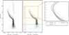 |
Fig. 2 Illustration of the photometric data used in this work. Left panel: the mF322W2 vs. mF115W − mF322W CMD, showing all detected stars. Likely SMC members and 47 Tucanae stars are marked with black and gray points, respectively. Right panel: the same CMD, restricted to stars in the field of the SMC. The black dashed line corresponds to the 50 % completeness limit for SMC stars in this dataset. The inset zooms in on the upper MS (20.4 < mF322W2 < 23.8), where three isochrones with an age of 7 Gyr, distance modulus (m − M)0 = 18.9, and reddening E(B − V) = 0.05 are overplotted. The blue and red lines correspond to metallicities of [Fe/H] = −2.2 and −0.5, while the green line indicates the best-fitting isochrone with [Fe/H] =−1.1. |
3.1 Binaries in the field of the Small Magellanic Cloud
The great distance to the SMC, namely ~60.3 kpc (see also Graczyk et al. 2020), prevents the direct resolution of individual components in binary systems, even with space-based telescopes such as the HST or the JWST. As a result, unresolved binaries appear as single sources in photometric observations. The total magnitude of an unresolved binary system is given by
 (1)
(1)
where m1 is the magnitude of the primary star, and F1 and F2 are the fluxes of the primary and secondary components, respectively.
In CMDs, unresolved binaries composed of two MS stars appear as point sources that are systematically redder and brighter than single MS stars. Their precise location in the CMD of a simple stellar population depends on the mass of the primary star and the mass ratio of the system, defined as q = M2 /M1. Systems with q ≈ 1, where the two stars have nearly equal masses, follow a sequence parallel to the MS but ~0.75 magnitudes brighter. Conversely, binaries with low mass ratios (q ~ 0) are nearly indistinguishable from single stars, as their combined flux remains close to the MS fiducial line. These effects are particularly relevant in the mF322W2 versus mF115W − mF322W2 CMD used in this study, where binaries predominantly populate the red and bright side of the MS fiducial sequence.
Over the past few decades, extensive investigations of binary systems in numerous Galactic and extragalactic star clusters have been carried out (e.g., Bolte 1992; Cool & Bolton 2002; Sollima et al. 2007, 2010; Cordoni et al. 2023; Mohandasan et al. 2024; Muratore et al. 2024; Bortolan et al. 2025). In the following, we estimate for the first time the fraction of photometric binary systems in the field of the SMC. To achieve this, we first approximated the SMC CMD as that of a simple stellar population and adapted the methodology introduced by Milone et al. (2012a) to our dataset. Our analysis focuses on binaries with mass ratios q > 0.6, as systems with lower mass ratios are located too close to the MS fiducial line to be reliably distinguished.
As illustrated in Fig. 3, we first identified two distinct regions in the mF322W2 versus mF115W − mF322W2 CMD. Region A (enclosed by the green solid line) includes both single MS stars with 22.5 ≤ mF322W2 ≤ 23.6 and binary systems where the primary star falls within the same magnitude range. The boundaries of region A are defined as follows: (i) the left boundary was obtained by shifting the MS fiducial line leftward by the average color error; (ii) the right boundary was obtained by shifting the equal-mass binary fiducial sequence rightward by twice the color uncertainty; and (iii) the upper and lower boundaries correspond to binary systems where the primary star has magnitudes mF322W2 = 22.5 and 23.6, respectively, covering the full range of possible mass ratios from q = 0 to q = 1. Region B is a subset of region A that is primarily populated by binaries with q > 0.6. Its left boundary is marked by the fiducial sequence of binary systems with q = 0.6 (orange continuous line), which serves as the threshold for our binary selection criteria.
The observed mF322W2 versus mF115W − mF322W2 CMD is presented in the left panel of Fig. 3. Candidate binary systems, identified as sources within region B, are marked with red crosses, while stars in region A are indicated with black points. The fraction of binaries with q > 0. 6 is computed as
 (2)
(2)
where  and
and  represent the number of observed stars, corrected for completeness, in region A and B, respectively.
  and
and  refer to the corresponding star counts in the AS CMD, shown in the central panel of Fig.3, while
  and
and  indicate the number of field stars within the selected regions. To evaluate the contribution of field stars, we compared the observed mF322W2 versus mF115W − mF322W2 CMD with a simulated CMD generated using the TRILEGAL code (Girardi et al. 2005). The simulation was performed for a Galactic field with the same area and Galactic coordinates as those of the field analyzed in this work. Simulated field stars are shown with azure starred symbols in the central panel of Fig. 3. The comparison indicates that Milky Way field star contamination of the SMC CMD sequence is negligible.
The resulting binary fraction in the field of the SMC is  . The uncertainties in each term of Eq. (2) are determined using Poisson statistics, while the total uncertainty in the binary fraction is derived through standard error propagation.
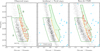 |
Fig. 3 Binary fraction estimation in the SMC field. Left panel: mF322W2 vs. mF115W − mF322W2 CMD of SMC stars. Region A (green solid line) includes MS stars and binaries with primary masses between 0.61 and 0.81 M⊙. Region B (green-shaded area) contains binaries with q > 0.6. MS and binary stars are indicated with black points and red crosses, respectively, while the remaining stars are colored in gray. Central panel: Same as the left panel but for artificial and field stars. Azure star symbols represent stars simulated with the TRILEGAL code (Girardi et al. 2005) within a Galactic field with the same area and coordinates as the one investigated in this work. Right panel: Best-fit simulated CMD. Colors and symbols follow the same scheme as in the left and central panels. |
3.2 Binaries and metallicity distribution
To assess whether the presence of stellar populations with distinct metallicities affects the measurement of the binary fraction in the SMC field, we compared the observed binary fraction from Sect. 3.1 with the corresponding fraction obtained from simulated CMDs that account for the metallicity distribution of SMC stars. The synthetic CMDs were generated through an iterative procedure consisting of the following steps.
First, we created a population of single stars by drawing [Fe/H] values from the SMC metallicity distribution derived by Mucciarelli et al. (2023), accounting also for the corresponding [α/Fe] relation reported by the same authors. Each star was then assigned a position in the CMD by linearly interpolating isochrones from the BaSTI stellar evolution models (Pietrinferni et al. 2021) across a grid of metallicities and [α/Fe] abundances. Next, we simulated binary systems following the method introduced by Milone et al. (2020), which has been extensively applied in previous studies (e.g., Muratore et al. 2024; Bortolan et al. 2025; Milone et al. 2025). In short, we generated binaries assuming a flat mass-ratio distribution and selected only those falling within the green-shaded region defined for observed stars. We then constructed a grid of simulated CMDs with binary fractions,  , ranging from 0.00 to 1.00 in steps of 0.01, with the corresponding fraction of single stars set to
  .
.
The binary fraction of each simulated CMD was measured using the same procedure described in Sect. 3.1 for real stars. We then compared the simulated values to observations via a χ2 minimization approach. In particular, χ2 has been defined as
 (3)
(3)
where nobs and nsim are the numbers of observed and simulated stars, respectively, that fall within region A and B.
The mF322W2 versus mF115W − mF322W2 CMD that provides the best match with the observations is illustrated in the right panel of Fig. 3.
The best-fitting model, corresponding to the minimum χ2 value, yields a binary fraction of  . To estimate the associated uncertainty, we generated 1000 synthetic CMDs assuming the best-fit binary fraction. For each simulation, we measured
  using the same approach as for real stars. The final uncertainty was computed as the root mean scatter of the 1000 individual values of
  .
.
To assess the impact of the adopted metallicity distribution (Mucciarelli et al. 2023), we repeated the entire procedure using a simplified metallicity distribution, where [Fe/H] values were uniformly drawn between −1.4 and −1.0 dex, as in Kalirai et al. (2013). Synthetic CMDs generated with this alternative distribution yielded a binary fraction of  , which is statistically consistent with the one derived using the empirical metallicity distribution. This indicates that the assumed metallicity distribution has a negligible effect on the derived binary fraction.
To compare our findings on SMC field stars with those for Galactic open clusters (OCs) and Milky Way field population, we show in Fig. 4 the fraction of binaries with q > 0.6,  as a function of the logarithm of the cluster age (panel a) and the total binary fraction3,
  , as a function of the primary star mass (panel b).
Values of  in Galactic OCs exhibit a mild correlation with the logarithm of the cluster age and no trend with the cluster metallicity, while the total binary fraction increases monotonically with primary mass. We found that the binary fraction in the SMC field is comparable to that observed in most Galactic OCs. Furthermore, our results align with the trend between total binary fraction and primary star mass reported for Galactic field stars suggesting that binary star formation and evolution in the low-metallicity environment of the SMC proceed similarly to those in low-density environments of the Milky Way.
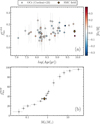 |
Fig. 4 Comparison of binary fractions in the SMC field and Galactic populations. Panel a: binary fraction with q > 0.6 as a function of the logarithm of cluster age. Galactic OCs are color-coded by their metallicity, as indicated by the colorbar on the right, while the orange diamond marks the binary fraction in the field of the SMC. The binary fractions and ages for OCs are from Cordoni et al. (2023) and Dias et al. (2021), respectively. Panel b: total binary fraction as a function of the mass of the primary star. Gray dots are taken from the review by Offner et al. (2023), and the orange diamond indicates the binary fraction measured for the SMC field in this work. |
3.3 Binaries and blue straggler stars
Blue straggler stars are observed as an extension of the MS in a region brighter and bluer than the turnoff in the mF322W2 versus mF115W − mF322W2 CMD. To identify them, we applied a selection method similar to Cordoni et al. (2023). Specifically, we defined two regions in the CMD, hereafter region C and region D. Region C corresponds to the area bounded by the zero-age MS isochrone (gray dashed line), the MS fiducial shifted blueward by five times the color uncertainty (blue solid line), and a vertical line at the color of the MS turnoff (azure dashed line). All stars located within this region were classified as candidate BSSs, resulting in the identification of 10 BSSs in the SMC field, marked as blue triangles in Fig. 5.
For region D, we adapted the definition by Cordoni et al. (2023) to the mF322W2 versus mF115W − mF322W2 CMD. Specifically, we identified region D as the interval included between the MS turnoff and one GRP magnitude below the MS turnoff, which, based on the best-fit isochrone, corresponds to 0.8 F322W2 magnitude. Its left boundary is set by the MS fiducial line shifted leftward by five times the color uncertainty, while the right boundary follows the fiducial of equal-mass binaries (red solid line).
The fraction of BSSs in the field of the SMC was estimated using the ratio
 (4)
(4)
where  and
and  represent the number of observed stars in regions C and D of the CMD, respectively, while
  and
and  are the corresponding quantities measured for field stars. The resulting BSS fraction in the field of the SMC is ƒBSS = 0.04 ± 0.01, similar to the values measured by Cordoni et al. (2023) in Galactic OCs, which range from 0.00 (no BSSs) up to 0.07. Alternatively, adopting the definition of region D from (Sollima et al. 2008, see their Sect. 3) we measured a lower BSS fraction, fBSS = 0.02 ± 0.01. Despite this difference, both measurements are compatible with those found in other low-density stellar environments, where mass transfer in binary systems is considered the dominant formation channel for BSSs (e.g., Momany et al. 2007; Cordoni et al. 2023).
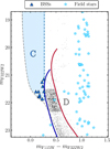 |
Fig. 5 Identification of candidate BSSs in the field of the SMC. The gray dashed line indicates the zero-age MS isochrone, and the azure dashed vertical line marks the color of the MS turnoff. The blue and red solid line represent the fiducial sequence of MS stars shifted blueward by five times the color error and the equal-mass binary fiducial, respectively. The azure-shaded area indicates region C, and region D is shown in gray. Candidate BSSs are highlighted with blue triangles, and field stars are shown as azure star symbols. See the main text for details. |
4 The initial mass function of field stars in the Small Magellanic Cloud
In the following, we derive the MF of field stars in the SMC. We begin by constructing the observed luminosity function, accounting for the presence of binaries (Sect. 4.1). In Sect. 4.2 we convert luminosities into stellar masses using the best-fit isochrone to obtain the MF. Finally, we determine the slope of the MF and discuss its implications for the universality of the IMF.
4.1 The luminosity function of field stars in the Small Magellanic Cloud
To derive the luminosity function of stars in the SMC field, we adapted the method introduced by Milone et al. (2012b) to our dataset. Panels a and b of Fig. 6 show the binning scheme used for the analysis. To properly account for binary contamination, we adopted different strategies for the upper and lower MS. Specifically, in the upper MS, we divided the CMD into five regions following a procedure similar to that described in Sect. 3.1. The key difference is that, for each of the five magnitude intervals, we only defined region A, namely the area enclosed by the green solid line in Fig. 3, which includes both single MS stars within a fixed 0.5 mag interval and binaries whose primary falls within the same range. Since binary identification in the mF322W2 versus mF115W − mF322W2 CMD is only reliable in the upper MS, we applied a uniform binning scheme with 0.5 mag-wide bins below the MS knee.
In both the upper and lower MS, observational errors cause contamination between adjacent bins, since stars can scatter into neighboring regions. As a result, the total number of stars observed in each region (corrected for completeness), Ni, can be expressed as
 (5)
(5)
where nk is the true number of stars in the k-th bin, and ck,i is the fraction of those stars scattered into the i-th bin due to observational uncertainties. The contamination matrix ck,i was computed using synthetic CMDs generated with ASs. The true star counts nk were then obtained by solving the linear system defined in Eq. (5).
To account for the presence of unresolved binaries, we first used the binary fraction with q < 0.6 measured in Sect. 3.1 to infer the total binary fraction,  . Assuming a flat mass-ratio distribution over the range 0 < q < 1, we derived
  . In each magnitude bin, we then randomly assigned binary companions by drawing mass ratios from a uniform distribution between q = 0 and q = 1. The corresponding companion masses were converted into F322W2 magnitudes using the mass–luminosity relation from Pietrinferni et al. (2021), and their flux contributions were added to the primary stars in the respective bins. The resulting luminosity function is shown in panel c of Fig. 6.
4.2 The mass function slope in the field of the Small Magellanic Cloud
Figure 6a shows the best-fitting isochrone from the BaSTI stellar evolution database (Pietrinferni et al. 2021). This fit adopts an age of 7 Gyr, a metallicity of [Fe/H] = −1.1, a distance modulus of (m − M)0 = 18.90, and a reddening of E(B−V) = 0.05. Using this isochrone, we converted the observed luminosities into stellar masses, as illustrated in the same panel. The distinct mass intervals used to construct the SMC MF are shown in different colors, with the average mass of stars in each bin labeled accordingly.
The resulting MF is shown in Fig. 6d, where we plot the logarithm of the number of stars per unit mass (log(dN/dM)), normalized by the bin width ΔM, as a function of the logarithm of stellar mass. A previous study by Kalirai et al. (2013), based on ultra-deep HST data, probed the MF of the SMC field down to M = 0.37 M⊙. In comparison, our JWST observations extend significantly deeper. According to our mass-luminosity relation, the faintest SMC stars detected in our data, at mF322W2 = 27.9, correspond to a mass of M = 0.11 M⊙. However, the 50% completeness limit occurs at mF322W2 = 26.22, which translates to M = 0.22 M⊙. This represents a substantial improvement in the ability to study the low-mass end of the SMC MF.
The present-day MF of the SMC field, expected to closely resemble the IMF given the dynamically mixed nature of field stars (Geha et al. 2013, and references therein), is commonly described by a power law
 (6)
(6)
where k is a normalization constant, and α is the slope. Taking the logarithm of both sides gives the linear form
 (7)
(7)
We performed a least-squares linear fit to the observed log(dN/dM) versus log(M) distribution, obtaining a best-fitting slope of α = −1.99 ± 0.08 (black solid line). To validate this result, we also estimated the MF slope using the maximum likelihood estimation approach, which assumes a power-law distribution with a lower mass limit Mmin and an infinite upper bound. Applying this method to the observed mass distribution yields αMLE = −1.85 ± 0.01, a value consistent with our least-squares estimate within 2σ.
Several studies have suggested that the stellar MF is better described by a broken power law. In particular, Kroupa (2001) reported a change in slope from α = −2.3 to α = −1.3 at M = 0.5 M⊙. When we imposed a break at M = 0.5 M⊙, we obtained α = −1.69 ± 0.15 for M < 0.5 M⊙ and α = −2.02 ± 0.29 for M > 0.5 M⊙. The high-mass slope agrees with the Kroupa value of α = −2.3, while the low-mass slope is slightly steeper than the α = −1.3 measured in the Galactic field, suggesting a relative deficit of low-mass stars in the SMC. Consistent with the findings of Kalirai et al. (2013), however, we find that a single power law reproduces the SMC field MF well and see no evidence of a broken MF in our data. Moreover, the broken power-law fit is statistically consistent with a single power law of slope α = −1.99 at 1σ level. Hence, in the following, we consider the value obtained from the entire mass range.
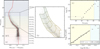 |
Fig. 6 Determination of the SMC MF. Panel a: mF322W2 vs. mF115W − mF322W2 CMD for stars in the SMC. The magnitude intervals are highlighted in different colors, with the corresponding average stellar masses labeled on the right. The red solid line shows the isochrone that best fits the observed stellar population. Panel b: zoom-in of the CMD focusing on the magnitude range 21.0 < mF322W2 < 24.3. Colored regions indicate the bins used to compute the MF along the upper MS, tailored to include binary stars. Panels c and d: mF322W2 luminosity function (panel c) and corresponding MF (panel d) for SMC field stars. White points mark bins with photometric completeness below 50%. In panel d, the black solid line represents a linear fit to the observed MF, restricted to regions of the CMD where the photometric completeness exceeds 50%. The derived MF slope is indicated in the bottom-right corner of the figure. In all panels, the gray dashed line indicates the 50% completeness limit. |
4.3 Comparison with previous studies
The MF slope, α, measured for the SMC field is shown in Fig. 7 alongside a broad compilation of MF slopes derived from various Galactic and extragalactic stellar populations. These include Galactic GCs (blue circles; Baumgardt et al. 2023), SMC and Large Magellanic Cloud (LMC) clusters (crimson triangles; Baumgardt et al. 2023), OCs (green thin crosses and green dashed lines; Ebrahimi et al. 2022; Cordoni et al. 2023)4, UFDs (gold squares; Geha et al. 2013; Gennaro et al. 2018a), the Milky Way field (gray diamonds; Reid et al. 1999, 2002; Schröder & Pagel 2003; Kroupa & Boily 2002; Allen et al. 2005; Metchev et al. 2008; Pinfield et al. 2008; Bochanski et al. 2010; Sollima 2019), the Galactic bulge (magenta starred symbol; Zoccali et al. 2000), and OB associations (cyan thick crosses; Reylé & Robin 2001; Schultheis et al. 2006; Vallenari et al. 2006).
Our SMC field measurement (orange diamond) extends down to 0.22 M⊙ at the 50% completeness limit, probing significantly lower stellar masses than most prior extragalactic studies. This enables a robust characterization of the MF in a low-metallicity, dynamically mixed stellar population. The resulting slope, α = −1.99 ± 0.08, is in excellent agreement with the value reported by Kalirai et al. (2013, cyan diamond),  , based on ultra-deep HST data over the mass range 0.37–0.93 M⊙.
In the context of broader stellar populations, the SMC slope is shallower than the canonical Salpeter value (red solid line). Additionally, it is consistent with the MF slopes observed in several Milky Way populations, including some OCs and GCs. Similarly, the SMC slope agrees with the values measured within SMC and LMC clusters, suggesting no strong variation in the MF between field and cluster environments at comparable metallicities.
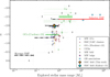 |
Fig. 7 MF slope, α, as a function of the explored stellar mass range, compiled from a variety of Galactic and extragalactic environments. Each point represents the best-fit power-law slope over a specific mass range, with horizontal error bars showing the width of the corresponding mass interval. Blue circles denote Milky Way GCs, crimson triangles SMC and LMC clusters, thin green crosses OCs, gold squares UFDs, gray diamonds Milky Way field stars, the magenta star the Galactic bulge, and thick cyan crosses OB associations. The orange diamond shows the measurement for the SMC field from this work, and the nearby cyan diamond corresponds to the result from Kalirai et al. (2013). The solid red line marks the canonical Salpeter (1955) IMF slope, and the dashed black lines represent the segmented IMF slopes from Kroupa (2001). The green dashed line corresponds to the slopes measured by Cordoni et al. (2023) for Galactic OCs. |
5 Summary and discussion
In this work we used deep JWST NIRCam photometry in the F115W and F322W2 bands to investigate stellar populations in the field of the SMC. Our study leveraged the unprecedented spatial resolution and depth of JWST observations to explore key aspects of stellar populations in a low-metallicity and low-density environment. Specifically, we primarily focused on measuring the fraction of binary systems and deriving the MF. These results provide valuable insights into the formation and evolution of stars in dwarf galaxies and contribute to ongoing discussions about the universality of the IMF. To properly account for binary contamination in the determination of the MF, we first concentrated on binaries:
We determined for the first time the fraction o0 unresolved binaries with mass ratios q > 0.6, finding
 . This value was independently confirmed through comparisons with synthetic CMDs that account for the SMC’s metallicity distribution, which yield a consistent value of
  ;
;We investigated the presence of BSSs in the CMD. In particular, we measured a BSS fraction of ƒBSS = 0.04 ± 0.01. This value is consistent with previous studies of BSSs in low-density stellar environments, such as dwarf spheroidal galaxies and GC outskirts, where dynamical interactions are rare and mass transfer in binary systems is believed to be the dominant formation channel (e.g., Momany et al. 2007; Ferraro et al. 2012). Notably, Cordoni et al. (2023) show that OCs also exhibit significant BSS populations with similar structural dependencies, reinforcing the idea that mass exchange in binaries is a universal mechanism shaping BSS formation, from sparse stellar systems like OCs to entire dwarf galaxies like the SMC.
The binary fraction measured for the SMC field in this work is comparable to that observed in Galactic OCs of similar ages. Furthermore, our result for the SMC field is consistent with the total binary fraction measured for Milky Way field stars of similar primary masses. These findings align with the general trend that binary fractions tend to be higher in lower-density environments, where dynamical interaction rates are relatively low. In contrast, Galactic GCs, characterized by much higher stellar densities and interaction rates, experience more frequent binary disruptions, resulting in systematically lower binary fractions (e.g., Sollima et al. 2007; Milone et al. 2012a, 2016). This comparison suggests that the binary star formation and evolutionary processes in the low-density environment of the SMC resemble those in Galactic OCs and field populations, supporting the notion that environmental density and dynamical interactions play a key role in shaping binary fractions across different stellar systems.
Our main results regarding the MF of the SMC field can be summarized as follows:
We constructed the luminosity function of SMC field stars and modeled it using synthetic populations that account for both completeness effects and unresolved binaries. Using the best-fit isochrone, we converted magnitudes to stellar masses; this allowed us to derive the MF down to M = 0.22 M⊙, significantly extending previous limits (Kalirai et al. 2013);
We measured the present-day MF of field stars in the SMC down to 0.22 M⊙, finding a power-law slope of α = −1.99 ± 0.08. This result provides an independent confirmation of the findings by Kalirai et al. (2013), who reported a slope of α = −1.90 over a narrower mass range (0.37–0.93 M⊙) in a different SMC field. Our measured slope is significantly shallower than the canonical Salpeter value (α = −2.35), challenging the notion of a universal IMF.
The shallower MF slope observed in the SMC implies that star formation in low-metallicity, low-density environments favors the formation of more intermediate- to high-mass stars compared to low-mass stars. This suggests that environmental conditions such as metallicity, temperature, and gas density influence the fragmentation of molecular clouds and the resulting stellar mass distribution. Such variations challenge the universality of the IMF and have important consequences for the chemical evolution, feedback, and dynamical history of dwarf galaxies like the SMC.
Acknowledgements
This work is based on observations made with the NASA/ESA/CSA James Webb Space Telescope. The data were obtained from the Mikulski Archive for Space Telescopes at the Space Telescope Science Institute, which is operated by the Association of Universities for Research in Astronomy, Inc., under NASA contract NAS 5-03127 for JWST. These observations are associated with program GO-2560. We thank the anonymous referee for various suggestions that improved the quality of the manuscript. This work has been funded by the European Union - NextGenerationEU RRF M4C2 1.1 (PRIN 2022 2022MMEB9W: “Understanding the formation of globular clusters with their multiple stellar generations”, CUP C53D23001200006) and from INAF Research GTO-Grant Normal RSN2-1.05.12.05.10 (PI A. F. Marino) of the “Bando INAF per il Finanziamento della Ricerca Fondamentale 2022”. T. Ziliotto acknowledges funding from the European Union’s Horizon 2020 research and innovation program under the Marie Skłodowska-Curie Grant Agreement No. 101034319 and from the “European Union – NextGenerationEU”.
References
- Abel, T., Bryan, G. L., & Norman, M. L. 2002, Science, 295, 93 [CrossRef] [Google Scholar]
- Allen, P. R., Koerner, D. W., Reid, I. N., & Trilling, D. E. 2005, ApJ, 625, 385 [Google Scholar]
- Almeida, L. A., Sana, H., Taylor, W., et al. 2017, A&A, 598, A84 [NASA ADS] [CrossRef] [EDP Sciences] [Google Scholar]
- Anderson, J., & King, I. R. 2006, PSFs, Photometry, and Astronomy for the ACS/WFC, Instrument Science Report ACS 2006-01, 34 [Google Scholar]
- Anderson, J., Sarajedini, A., Bedin, L. R., et al. 2008, AJ, 135, 2055 [Google Scholar]
- Baumgardt, H., Hénault-Brunet, V., Dickson, N., & Sollima, A. 2023, MNRAS, 521, 3991 [CrossRef] [Google Scholar]
- Bellini, A., Anderson, J., Bedin, L. R., et al. 2017, ApJ, 842, 6 [NASA ADS] [CrossRef] [Google Scholar]
- Bochanski, J. J., Hawley, S. L., Covey, K. R., et al. 2010, AJ, 139, 2679 [NASA ADS] [CrossRef] [Google Scholar]
- Bolte, M. 1992, ApJS, 82, 145 [NASA ADS] [CrossRef] [Google Scholar]
- Bortolan, E., Bruce, J., Milone, A. P., et al. 2025, A&A, 696, A220 [NASA ADS] [CrossRef] [EDP Sciences] [Google Scholar]
- Bromm, V., Coppi, P. S., & Larson, R. B. 2002, ApJ, 564, 23 [Google Scholar]
- Cappellari, M., McDermid, R. M., Alatalo, K., et al. 2012, Nature, 484, 485 [Google Scholar]
- Carrera, R., Gallart, C., Aparicio, A., et al. 2008, AJ, 136, 1039 [Google Scholar]
- Choudhury, S., de Grijs, R., Rubele, S., et al. 2020, MNRAS, 497, 3746 [NASA ADS] [CrossRef] [Google Scholar]
- Conroy, C., & van Dokkum, P. G. 2012, ApJ, 760, 71 [Google Scholar]
- Cool, A. M., & Bolton, A. S. 2002, in Astronomical Society of the Pacific Conference Series, 263, Stellar Collisions, Mergers and their Consequences, ed. M. M. Shara, 163 [Google Scholar]
- Cordoni, G., Milone, A. P., Marino, A. F., et al. 2023, A&A, 672, A29 [NASA ADS] [CrossRef] [EDP Sciences] [Google Scholar]
- Dias, W. S., Monteiro, H., Moitinho, A., et al. 2021, MNRAS, 504, 356 [NASA ADS] [CrossRef] [Google Scholar]
- Dobbie, P. D., Cole, A. A., Subramaniam, A., & Keller, S. 2014a, MNRAS, 442, 1663 [Google Scholar]
- Dobbie, P. D., Cole, A. A., Subramaniam, A., & Keller, S. 2014b, MNRAS, 442, 1680 [NASA ADS] [CrossRef] [Google Scholar]
- Dondoglio, E., Milone, A. P., Renzini, A., et al. 2022, ApJ, 927, 207 [NASA ADS] [CrossRef] [Google Scholar]
- Dunstall, P. R., Dufton, P. L., Sana, H., et al. 2015, A&A, 580, A93 [NASA ADS] [CrossRef] [EDP Sciences] [Google Scholar]
- Ebrahimi, H., Sollima, A., & Haghi, H. 2022, MNRAS, 516, 5637 [NASA ADS] [CrossRef] [Google Scholar]
- Ferraro, F. R., Lanzoni, B., Dalessandro, E., et al. 2012, Nature, 492, 393 [Google Scholar]
- Geha, M., Brown, T. M., Tumlinson, J., et al. 2013, ApJ, 771, 29 [NASA ADS] [CrossRef] [Google Scholar]
- Gennaro, M., Geha, M., Tchernyshyov, K., et al. 2018a, ApJ, 863, 38 [NASA ADS] [CrossRef] [Google Scholar]
- Gennaro, M., Tchernyshyov, K., Brown, T. M., et al. 2018b, ApJ, 855, 20 [NASA ADS] [CrossRef] [Google Scholar]
- Girardi, L., Groenewegen, M. A. T., Hatziminaoglou, E., & da Costa, L. 2005, A&A, 436, 895 [NASA ADS] [CrossRef] [EDP Sciences] [Google Scholar]
- Graczyk, D., Pietrzynski, G., Thompson, I. B., et al. 2020, ApJ, 904, 13 [Google Scholar]
- Kalirai, J. S., Anderson, J., Dotter, A., et al. 2013, ApJ, 763, 110 [NASA ADS] [CrossRef] [Google Scholar]
- Kalari, V. M., Vink, J. S., Dufton, P. L., & Fraser, M. 2018, A&A, 618, A17 [NASA ADS] [CrossRef] [EDP Sciences] [Google Scholar]
- Kroupa, P. 2001, MNRAS, 322, 231 [NASA ADS] [CrossRef] [Google Scholar]
- Kroupa, P., & Boily, C. M. 2002, MNRAS, 336, 1188 [Google Scholar]
- Legnardi, M. V., Milone, A. P., Cordoni, G., et al. 2023, MNRAS, 522, 367 [CrossRef] [Google Scholar]
- Luhman, K. L., Mamajek, E. E., Allen, P. R., & Cruz, K. L. 2009, ApJ, 703, 399 [NASA ADS] [CrossRef] [Google Scholar]
- Mackey, D., Koposov, S., Da Costa, G., et al. 2018, ApJ, 858, L21 [Google Scholar]
- Marino, A. F., Milone, A. P., Legnardi, M. V., et al. 2024a, ApJ, 965, 189 [NASA ADS] [CrossRef] [Google Scholar]
- Marino, A. F., Milone, A. P., Renzini, A., et al. 2024b, ApJ, 969, L8 [Google Scholar]
- Metchev, S. A., Kirkpatrick, J. D., Berriman, G. B., & Looper, D. 2008, ApJ, 676, 1281 [Google Scholar]
- Milone, A. P., Piotto, G., Bedin, L. R., et al. 2012a, A&A, 540, A16 [NASA ADS] [CrossRef] [EDP Sciences] [Google Scholar]
- Milone, A. P., Piotto, G., Bedin, L. R., et al. 2012b, A&A, 537, A77 [NASA ADS] [CrossRef] [EDP Sciences] [Google Scholar]
- Milone, A. P., Marino, A. F., Bedin, L. R., et al. 2016, MNRAS, 455, 3009 [CrossRef] [Google Scholar]
- Milone, A. P., Vesperini, E., Marino, A. F., et al. 2020, MNRAS, 492, 5457 [Google Scholar]
- Milone, A. P., Cordoni, G., Marino, A. F., et al. 2023a, A&A, 672, A161 [NASA ADS] [CrossRef] [EDP Sciences] [Google Scholar]
- Milone, A. P., Marino, A. F., Dotter, A., et al. 2023b, MNRAS, 522, 2429 [CrossRef] [Google Scholar]
- Milone, A. P., Marino, A. F., Bernizzoni, M., et al. 2025, A&A, 698, A247 [NASA ADS] [CrossRef] [EDP Sciences] [Google Scholar]
- Mohandasan, A., Milone, A. P., Cordoni, G., et al. 2024, A&A, 681, A42 [NASA ADS] [CrossRef] [EDP Sciences] [Google Scholar]
- Momany, Y., Held, E. V., Saviane, I., et al. 2007, A&A, 468, 973 [NASA ADS] [CrossRef] [EDP Sciences] [Google Scholar]
- Mucciarelli, A., Minelli, A., Bellazzini, M., et al. 2023, A&A, 671, A124 [NASA ADS] [CrossRef] [EDP Sciences] [Google Scholar]
- Muratore, F., Milone, A. P., D’Antona, F., et al. 2024, A&A, 692, A135 [NASA ADS] [CrossRef] [EDP Sciences] [Google Scholar]
- Nardiello, D., Libralato, M., Piotto, G., et al. 2018, MNRAS, 481, 3382 [NASA ADS] [CrossRef] [Google Scholar]
- Offner, S. S. R., Moe, M., Kratter, K. M., et al. 2023, in Astronomical Society of the Pacific Conference Series, 534, Protostars and Planets VII, eds. S. Inutsuka, Y. Aikawa, T. Muto, K. Tomida, & M. Tamura, 275 [NASA ADS] [Google Scholar]
- Pastorelli, G., Marigo, P., Girardi, L., et al. 2019, MNRAS, 485, 5666 [Google Scholar]
- Piatti, A. E. 2021, A&A, 650, A52 [NASA ADS] [CrossRef] [EDP Sciences] [Google Scholar]
- Pietrinferni, A., Hidalgo, S., Cassisi, S., et al. 2021, ApJ, 908, 102 [NASA ADS] [CrossRef] [Google Scholar]
- Pinfield, D. J., Burningham, B., Tamura, M., et al. 2008, MNRAS, 390, 304 [Google Scholar]
- Pouteau, Y., Motte, F., Nony, T., et al. 2022, A&A, 664, A26 [NASA ADS] [CrossRef] [EDP Sciences] [Google Scholar]
- Reid, I. N., Kirkpatrick, J. D., Liebert, J., et al. 1999, ApJ, 521, 613 [Google Scholar]
- Reid, I. N., Gizis, J. E., & Hawley, S. L. 2002, AJ, 124, 2721 [NASA ADS] [CrossRef] [Google Scholar]
- Reylé, C., & Robin, A. C. 2001, A&A, 373, 886 [NASA ADS] [CrossRef] [EDP Sciences] [Google Scholar]
- Rubele, S., Pastorelli, G., Girardi, L., et al. 2018, MNRAS, 478, 5017 [NASA ADS] [CrossRef] [Google Scholar]
- Sabbi, E., Gallagher, J. S., Tosi, M., et al. 2009, ApJ, 703, 721 [NASA ADS] [CrossRef] [Google Scholar]
- Sabbi, E., Lennon, D. J., Anderson, J., et al. 2016, ApJS, 222, 11 [NASA ADS] [CrossRef] [Google Scholar]
- Salpeter, E. E. 1955, ApJ, 121, 161 [Google Scholar]
- Schneider, F. R. N., Sana, H., Evans, C. J., et al. 2018, Science, 359, 69 [NASA ADS] [CrossRef] [Google Scholar]
- Schröder, K. P., & Pagel, B. E. J. 2003, MNRAS, 343, 1231 [Google Scholar]
- Schultheis, M., Robin, A. C., Reylé, C., et al. 2006, A&A, 447, 185 [NASA ADS] [CrossRef] [EDP Sciences] [Google Scholar]
- Sollima, A. 2019, MNRAS, 489, 2377 [NASA ADS] [CrossRef] [Google Scholar]
- Sollima, A., & Baumgardt, H. 2017, MNRAS, 471, 3668 [NASA ADS] [CrossRef] [Google Scholar]
- Sollima, A., Beccari, G., Ferraro, F. R., Fusi Pecci, F., & Sarajedini, A. 2007, MNRAS, 380, 781 [NASA ADS] [CrossRef] [Google Scholar]
- Sollima, A., Lanzoni, B., Beccari, G., Ferraro, F. R., & Fusi Pecci, F. 2008, A&A, 481, 701 [NASA ADS] [CrossRef] [EDP Sciences] [Google Scholar]
- Sollima, A., Carballo-Bello, J. A., Beccari, G., et al. 2010, MNRAS, 401, 577 [NASA ADS] [CrossRef] [Google Scholar]
- Vallenari, A., Pasetto, S., Bertelli, G., et al. 2006, A&A, 451, 125 [NASA ADS] [CrossRef] [EDP Sciences] [Google Scholar]
- van Dokkum, P. G., & Conroy, C. 2010, Nature, 468, 940 [Google Scholar]
- Wyse, R. F. G., Gilmore, G., Houdashelt, M. L., et al. 2002, New A, 7, 395 [Google Scholar]
- Zoccali, M., Cassisi, S., Frogel, J. A., et al. 2000, ApJ, 530, 418 [NASA ADS] [CrossRef] [Google Scholar]
Mucciarelli et al. (2023) analyzed spectra of over 300 stars in three SMC fields centered on the clusters NGC 121 (FLD-121), NGC 339 (FLD-339), and NGC 419 (FLD-419). FLD-121 (α ~ 00h26m49.0s, δ ~ −71d32m09.9s), FLD-339 (α ~ 00h57m48.9s, δ ~ −74d28m00.1s), and FLD-419 (α ~ 01h08m17.7s, δ ~ − 72d53m02.7s) are located ~2.5° northwest, ~1.4° southeast, and ~1.5° east of the SMC center, respectively.
We extrapolated the value of the total binary fraction,  , from the
  by assuming a flat mass-ratio distribution over the range 0 < q < 1.
As in Baumgardt et al. (2023), we only show clusters with life-times and relaxation times larger than their ages. For these objects, the present-day MF should still reflect the initial one.
All Figures
|
Fig. 1 Image of the SMC obtained from the Digitized Sky Survey 2. The inset provides a close-up view of the region near 47 Tucanae where the observations for this study were carried out. The NIRCam field of view analyzed in this work is outlined in green, and the footprints of the observations used by Kalirai et al. (2013) are shown in red. The white cross marks the position of the SMC center (Piatti 2021). North is up, and east is to the left. |
| In the text | |
|
Fig. 2 Illustration of the photometric data used in this work. Left panel: the mF322W2 vs. mF115W − mF322W CMD, showing all detected stars. Likely SMC members and 47 Tucanae stars are marked with black and gray points, respectively. Right panel: the same CMD, restricted to stars in the field of the SMC. The black dashed line corresponds to the 50 % completeness limit for SMC stars in this dataset. The inset zooms in on the upper MS (20.4 < mF322W2 < 23.8), where three isochrones with an age of 7 Gyr, distance modulus (m − M)0 = 18.9, and reddening E(B − V) = 0.05 are overplotted. The blue and red lines correspond to metallicities of [Fe/H] = −2.2 and −0.5, while the green line indicates the best-fitting isochrone with [Fe/H] =−1.1. |
| In the text | |
|
Fig. 3 Binary fraction estimation in the SMC field. Left panel: mF322W2 vs. mF115W − mF322W2 CMD of SMC stars. Region A (green solid line) includes MS stars and binaries with primary masses between 0.61 and 0.81 M⊙. Region B (green-shaded area) contains binaries with q > 0.6. MS and binary stars are indicated with black points and red crosses, respectively, while the remaining stars are colored in gray. Central panel: Same as the left panel but for artificial and field stars. Azure star symbols represent stars simulated with the TRILEGAL code (Girardi et al. 2005) within a Galactic field with the same area and coordinates as the one investigated in this work. Right panel: Best-fit simulated CMD. Colors and symbols follow the same scheme as in the left and central panels. |
| In the text | |
|
Fig. 4 Comparison of binary fractions in the SMC field and Galactic populations. Panel a: binary fraction with q > 0.6 as a function of the logarithm of cluster age. Galactic OCs are color-coded by their metallicity, as indicated by the colorbar on the right, while the orange diamond marks the binary fraction in the field of the SMC. The binary fractions and ages for OCs are from Cordoni et al. (2023) and Dias et al. (2021), respectively. Panel b: total binary fraction as a function of the mass of the primary star. Gray dots are taken from the review by Offner et al. (2023), and the orange diamond indicates the binary fraction measured for the SMC field in this work. |
| In the text | |
|
Fig. 5 Identification of candidate BSSs in the field of the SMC. The gray dashed line indicates the zero-age MS isochrone, and the azure dashed vertical line marks the color of the MS turnoff. The blue and red solid line represent the fiducial sequence of MS stars shifted blueward by five times the color error and the equal-mass binary fiducial, respectively. The azure-shaded area indicates region C, and region D is shown in gray. Candidate BSSs are highlighted with blue triangles, and field stars are shown as azure star symbols. See the main text for details. |
| In the text | |
|
Fig. 6 Determination of the SMC MF. Panel a: mF322W2 vs. mF115W − mF322W2 CMD for stars in the SMC. The magnitude intervals are highlighted in different colors, with the corresponding average stellar masses labeled on the right. The red solid line shows the isochrone that best fits the observed stellar population. Panel b: zoom-in of the CMD focusing on the magnitude range 21.0 < mF322W2 < 24.3. Colored regions indicate the bins used to compute the MF along the upper MS, tailored to include binary stars. Panels c and d: mF322W2 luminosity function (panel c) and corresponding MF (panel d) for SMC field stars. White points mark bins with photometric completeness below 50%. In panel d, the black solid line represents a linear fit to the observed MF, restricted to regions of the CMD where the photometric completeness exceeds 50%. The derived MF slope is indicated in the bottom-right corner of the figure. In all panels, the gray dashed line indicates the 50% completeness limit. |
| In the text | |
|
Fig. 7 MF slope, α, as a function of the explored stellar mass range, compiled from a variety of Galactic and extragalactic environments. Each point represents the best-fit power-law slope over a specific mass range, with horizontal error bars showing the width of the corresponding mass interval. Blue circles denote Milky Way GCs, crimson triangles SMC and LMC clusters, thin green crosses OCs, gold squares UFDs, gray diamonds Milky Way field stars, the magenta star the Galactic bulge, and thick cyan crosses OB associations. The orange diamond shows the measurement for the SMC field from this work, and the nearby cyan diamond corresponds to the result from Kalirai et al. (2013). The solid red line marks the canonical Salpeter (1955) IMF slope, and the dashed black lines represent the segmented IMF slopes from Kroupa (2001). The green dashed line corresponds to the slopes measured by Cordoni et al. (2023) for Galactic OCs. |
| In the text | |
Current usage metrics show cumulative count of Article Views (full-text article views including HTML views, PDF and ePub downloads, according to the available data) and Abstracts Views on Vision4Press platform.
Data correspond to usage on the plateform after 2015. The current usage metrics is available 48-96 hours after online publication and is updated daily on week days.
Initial download of the metrics may take a while.