| Issue |
A&A
Volume 702, October 2025
|
|
|---|---|---|
| Article Number | A216 | |
| Number of page(s) | 8 | |
| Section | Stellar structure and evolution | |
| DOI | https://doi.org/10.1051/0004-6361/202556527 | |
| Published online | 24 October 2025 | |
Propeller effect in action: Unveiling quenched accretion in the transient X-ray pulsar 4U 0115+63
1
Department of Physics and Astronomy, FI-20014 University of Turku, Finland
2
Institut für Astronomie und Astrophysik, Universität Tübingen, Sand 1, D-72076 Tübingen, Germany
3
Astrophysics, Department of Physics, University of Oxford, Denys Wilkinson Building, Keble Road, Oxford OX1 3RH, UK
4
School of Physics and Astronomy, Sun Yat-sen University, Zhuhai 519082, PR China
5
CSST Science Center for the Guangdong-Hong Kong-Macau Greater Bay Area, DaXue Road 2, 519082 Zhuhai, PR China
⋆ Corresponding author: This email address is being protected from spambots. You need JavaScript enabled to view it.
Received:
21
July
2025
Accepted:
10
September
2025
Abstract
The Be/X-ray pulsar 4U 0115+63 underwent a type II outburst in 2023. After the outburst, similar to the outbursts in 2015 and 2017, the source decayed into a quiescent state. Two out of three XMM-Newton observations conducted after the 2023 outburst confirmed the source to be in a low-luminosity state at a level of LX ∼ 1033 erg s−1. X-ray pulsations were detected at ≈0.277 Hz in both observations with a pulsed fraction exceeding 50%. The power density spectra show no significant low-frequency red noise in either observation, suggesting that the radiation is not driven by accretion. The energy spectra in this state can be described by a single blackbody component, with an emitting area smaller than the typical size of the polar caps during the accretion phase. Based on the timing and spectral properties, we suggest that the propeller effect is active during the quiescent state, resulting in a total quenching of accretion. We discuss possible mechanisms for the generation of pulsations in this regime and consider the scenario of neutron star crust cooling.
Key words: accretion / accretion disks / pulsars: general / X-rays: binaries / X-rays: individuals: 4U 0115+63
© The Authors 2025
 Open Access article, published by EDP Sciences, under the terms of the Creative Commons Attribution License (https://creativecommons.org/licenses/by/4.0), which permits unrestricted use, distribution, and reproduction in any medium, provided the original work is properly cited.
This article is published in open access under the Subscribe to Open model. This email address is being protected from spambots. You need JavaScript enabled to view it. to support open access publication.
1. Introduction
Transient X-ray pulsars (XRPs) in Be X-ray binaries (BeXRPs) host a highly magnetized neutron star (NS) with a magnetic field on the order of B ∼ 1012 − 1013 G. BeXRPs emit X-rays when accreting matter from a decretion disk that episodically forms around a rapidly rotating Be-type companion star. As the accreted material approaches the NS magnetosphere, it couples to the magnetic field lines and is funneled onto the magnetic poles. This process releases gravitational potential energy, which is radiated as X-rays. The anisotropic nature of the accretion flow leads to pulsed X-ray emission modulated by the NS rotation (for a review, see Mushtukov & Tsygankov 2024). These systems usually have significantly eccentric orbits. Near periastron, the increase in the mass accretion rate can trigger a so-called type I outburst, with X-ray luminosities reaching up to LX ∼ 1037 erg s−1. In other cases, BeXRPs can reach luminosities above the Eddington limit for a NS during giant (type II) outbursts. The physical mechanism behind type II outbursts remains uncertain (see the review by Reig 2011).
The temporal evolution of the observed X-ray flux from transient XRPs is governed to a large extent by the interaction of matter with the magnetic field. For instance, for the systems with fast-spinning NSs (typical spin period Pspin ≲ 10 s), at the end of the outburst, when the mass accretion rate decreases to a threshold value, the accretion is expected to be inhibited by the centrifugal barrier – the so-called propeller regime (Illarionov & Sunyaev 1975). The threshold mass accretion rate corresponding to the transition to the propeller regime corresponds to the equality of the magnetospheric and corotation radii of the NS and can be expressed as (e.g., Stella et al. 1986)

where B12 is the magnetic field strength in units of 1012 G, Pspin is the spin period in seconds, M1.4 is the NS mass in units of 1.4 M⊙, R6 is the radius in 106 cm, and k is a geometric factor of order unity. Below this luminosity threshold, accretion onto the NS is expected to cease abruptly, resulting in a sharp decline in observed flux and a transition to a low-luminosity quiescent state. In several XRPs, dramatic luminosity evolutions have been observed in the final stages of their outbursts and are considered to result from the propeller effect, for example SXP 4.78 (Semena et al. 2019), GRO J1750−27 (Lutovinov et al. 2019), 4U 0115+63, and V 0332+53 (Stella et al. 1986; Campana et al. 2001; Tsygankov et al. 2016).
At the same time, most transient XRPs observed in quiescence exhibit a nonzero flux in the X-ray band, with a typical luminosity of L0.5 − 10 keV ≲ 1034 erg s−1 (Tsygankov et al. 2017a). Moreover, some sources still display pulsations during this state (e.g., 4U 1145−619, Mukherjee & Paul 2005; 1A 1118−615, Rutledge et al. 2007; 1A 0535+262, Mukherjee & Paul 2005; and 4U 0115+63, Rouco Escorial et al. 2017, 2020; see also Table 1 in Tsygankov et al. 2017a for a complete source list). The reason for this phenomenon remains unknown, with two main hypotheses proposed. The first is the leakage of matter through the centrifugal barrier along magnetic field lines, which leads to the formation of hot spots (see, e.g., Elsner & Lamb 1977; Ikhsanov 2001; Lii et al. 2014; Orlandini et al. 2004; Mukherjee & Paul 2005). The second is thermal emission from a cooling, accretion-heated NS, in which more heat from the solid crustal layer is conducted to the magnetic poles due to anisotropic heat transport governed by the magnetic field lines (Rouco Escorial et al. 2017).
Therefore, the possibility of accretion onto the NS surface in the propeller regime remains viable and has not been definitively ruled out by observational data. Determining the origin of the emission in the quiescent state of a transient XRP requires high-quality data obtained during this phase. Such data were acquired with the XMM-Newton observatory for the well-studied pulsar 4U 0115+63 following its 2023 outburst.
4U 0115+63 is a typical transient BeXRP that was discovered by the Uhuru satellite (Giacconi et al. 1972) and identified as having a B0.2Ve spectral type companion star (Johns et al. 1978). The NS has a magnetic field strength B ≈ 1.3 × 10¹² G as measured from the cyclotron line energy (Heindl et al. 2000) a spin period Pspin ≈ 3.61 s (Cominsky et al. 1978). It orbits its companion every 24.3 d with an eccentricity of approximately 0.34 (Rappaport et al. 1978). The distance to the source is estimated to be ≈5.0 kpc, based on the Gaia data (Neumann et al. 2023).
Over the last decade, 4U 0115+63 has experienced several giant type II outbursts. Tsygankov et al. (2016) discovered a rapid drop in flux following the 2015 outburst and suggested that the source had transitioned into the propeller regime. The authors estimated the threshold luminosity for this transition to be (1.4 ± 0.4)×1036 erg s−1. Based on follow-up observations using Swift and XMM-Newton at the end of this and the following outbursts, the source was found to be in a low-luminosity state with L0.5 − 10 keV ∼ 1033 erg s−1 (Wijnands & Degenaar 2016; Rouco Escorial et al. 2017, 2020). X-ray pulsations were detected in the XMM-Newton observations during this state (Rouco Escorial et al. 2017, 2020).
In this study we performed timing and spectral analysis of the deep XMM-Newton observations of 4U 0115+63 obtained after the 2023 giant outburst to constrain the origin of its pulsating emission in the quiescent state.
2. Observations and data reduction
In March 2023, 4U 0115+63 exhibited a new type II outburst, followed by a decay into a low-luminosity (quiescent) state. XMM-Newton observed the source multiple times, and we used the suitable data from the XMM European Photon Imaging Camera (EPIC), Specifically, EPIC-PN (hereafter PN) and EPIC-MOS (hereafter MOS) detectors. Observations were conducted on 2023 July 13 (MJD 60138, hereafter Obs1), August 4 (MJD 60160, Obs2), and September 11 (MJD 60198, Obs3). We also included an observation conducted on 2016 February 17 (MJD 57435; Obs2016), when the source was in the quiescence (see Table 1 and Fig. 1 for details).
Details of the XMM-Newton observations of 4U 0115+63 used in this paper.
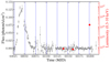 |
Fig. 1. Light curves of 4U 0115+63 during and after the 2023 giant outburst observed with Swift/BAT (gray) and XMM-Newton (red). The luminosities of XMM-Newton observations in the 0.3−10 keV band are |
Following the official SAS Science threads1, the data reduction was performed by using the Science Analysis System (SAS v22.1.0)2 software with the latest calibration datasets. We used the epproc and emproc tasks to produce calibrated and concatenated event lists from the PN and MOS cameras, respectively. To remove high background flaring activity from the observations, the single-event (PATTERN= = 0) light curves in the 10−12 keV band for the PN camera and > 10 keV for the MOS cameras were extracted; then we used the threshold rates for a steady low background (see Table 1) to get the good time intervals of each observation. Due to the very low count rates of the source during the XMM-Newton observations, Obs1, Obs2, and Obs2016 were not affected by pile-up. For these observations, the source region was identified as a circular region with a 20″ radius, and the background was extracted from a nearby, source-free circular region with a 50″ radius on the same CCD. For Obs3, to mitigate pile-up effects, we used an annular source region centered on the source position, with an inner radius of 10″ and an outer radius of 20″. We extracted the single and double events (PATTERN ≤ 4) for the PN camera and the events between single and quadruple (PATTERN ≤ 12) for the MOS cameras. The barycentric correction was performed by using barycen task.
For the timing analysis, we used the epiclccorr task to obtain net light curves. We used the powspec tool to get the power density spectra (PDSs) and folded the pulse profiles using the efold tool from the HEASoft v6.35.1 package3. The background spectra were scaled using the backscale task. The response matrix and the ancillary response files were generated using rmfgen and arfgen, respectively. We used the epicspeccombine task to combine the spectra of three EPIC cameras in order to improve statistics. Due to the very few counts in the spectra, we re-binned the spectra with grppha tool to make sure each bin has a minimum count of 5. The spectral analysis was performed by using the X-ray spectral fitting package (XSPEC) version 12.15.0 (Arnaud 1996). We used C-statistics for the statistics of fitting. All uncertainties in this paper for spectral analysis correspond to a confidence level of 90%, estimated by running Monte Carlo Markov chains with a length of 20 000 with a burn-in of 10 000 using the Goodman-Weare algorithm.
3. Results
Discriminating between accretion and cooling scenarios for the observed emission from a transient XRP in the quiescent state can be achieved by analyzing both the timing and spectral properties of its emission.
3.1. Timing analysis
X-ray pulsations from 4U 0115+63 during its quiescent states have been detected after the 2015 and 2017 giant outbursts (Rouco Escorial et al. 2017, 2020). To search for possible periodic signals associated with the NS spin in the data obtained during the 2023 outburst (see Table 1), we extracted the background subtracted PN light curves in 0.3−10 keV band with a bin size of 0.1 s and calculated their Lomb-Scargle periodograms (Lomb 1976; Scargle 1982) in 0.1−0.5 Hz range using the PYTHON package ASTROPY. The results are shown is Fig. 2. We did not use the data from the MOS cameras in the timing analysis due to their poor time resolution (2.6 s in full frame mode)4. The Lomb-Scargle periodograms show significant signals at ≈0.277 Hz in all three observations, corresponding to the NS spin frequency. We examined the confidence levels of these periodic signals, resulting in false alarm probabilities of 2.8 × 10⁻⁵, 4 × 10⁻³, and 3.2 × 10−209 for Obs1, Obs2, and Obs3, respectively. The corresponding pulse periods were precisely estimated using the Z2 method (Buccheri et al. 1983) in STINGRAY (Huppenkothen et al. 2019) package to be 3.6136 ± 0.0003 s, 3.6143 ± 0.0003 s, and 3.61339 ± 0.00005 s, respectively, where the uncertainties correspond to the standard deviation.
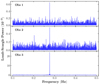 |
Fig. 2. Lomb-Scargle periodograms of 4U 0115+63 derived from three background-subtracted light curves with 0.1 s bins, observed by XMM-Newton in 2023. Clear pulsations are detected at a frequency of ≈0.277 Hz, corresponding to the NS spin frequency. |
In accreting systems like XRPs, accretion is an intrinsically noisy process, where fluctuations in the mass accretion rate are driven by random variations in the viscosity within the accretion disk (Lyubarskii 1997). Therefore, if accretion is the primary mechanism responsible for the observed X-ray emission, a feasible way to validate this process is by studying the aperiodic variability in the light curves (e.g., Doroshenko et al. 2020). Specifically, the authors compared the PDSs of accreting pulsars and non-accreting systems (such as magnetars and radio pulsars), showing that low-frequency noise dominates the PDSs of accreting systems. They attributed these differences to the presence or absence of ongoing accretion onto the NS.
To test for the presence of accretion in 4U 0115+63 during the different states observed with XMM-Newton, we generated PDSs using the powspec tool from the HEASoft package, as shown in Fig. 3. We note that the XMM-Newton observation from 2016 (Obs2016) shows an averaged count rate similar to that of Obs1 and Obs2 (Rouco Escorial et al. 2020). Therefore, we included this observation in the timing and spectral analysis to improve the statistics. As clearly seen in Fig. 3, the red noise dominates the low-frequency part of the PDS in Obs3. This observation was performed when the NS was near periastron passage (see Fig. 1), a phase where the system is expected to experience an increased accretion rate, potentially leading to a type I outburst. In contrast, the PDS of the merged light curves from Obs1, Obs2, and Obs2016 remains flat at a level of ∼2 at low frequencies, which is characteristic of the white noise. We fitted this PDS with a constant value of 2, yielding a reduced chi-square of χred2 = 0.82 with 511 degrees of freedom. At the same time, peaks in the PDS corresponding to the spin frequency are significantly detected at ≈0.277 Hz in both states. We fitted both peaks with a Gaussian function, resulting in a standard deviation of 3 × 10⁻⁴ Hz for the quiescent observations, whereas the peak in Obs3 appears broadened with a higher standard deviation of 1 × 10⁻³ Hz, likely due to the interplay between periodic and aperiodic variability.
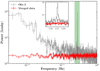 |
Fig. 3. PDSs of 4U 0115+63 normalized as in Leahy et al. (1983) and obtained using 0.1 s binned, background-subtracted light curves. The gray step line represents the PDS from Obs3, which clearly shows a red noise component at low frequencies. The red step line corresponds to the PDS from the combined light curves of Obs1, Obs2, and Obs2016, which exhibits a flat (white noise) distribution in the 0.003−1 Hz range. The inset provides a zoomed-in view around the NS spin frequency (highlighted by the green stripe). |
The pulse profiles of 4U 0115+63 obtained when the source was in the quiescent (Obs1, Obs2, and Obs2016) and accreting states (Obs3) are shown in Fig. 4. For the quiescence, the pulse profiles are very similar, consisting of a sinusoidal-like peak accompanied by a weak harmonic, consistent with the findings of Rouco Escorial et al. (2020). The averaged pulse profile was fitted with a combination of a sinusoid and its first harmonic, revealing an amplitude ratio between the fundamental and harmonic of approximately 3. We quantified the pulse amplitude using the fractional root-mean-square pulsed fraction (PF), which is defined as
 (1)
(1)
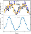 |
Fig. 4. Pulse profiles from the XMM-Newton observations obtained during the quiescent (top) and accreting (bottom) states of 4U 0115+63, folded using background-subtracted light curves with 0.1 s binning in the 0.3−10 keV energy range and using spin periods estimated via epoch-folding. The profiles were normalized by their average count rates. Phases were aligned using the cross-correlation method. |
where N represents the number of phase bins, ri is the count rate in the i-th phase bin, and  is the phase-averaged count rate. The resulting PF values for Obs1, Obs2, and Obs2016 are 52 ± 5%, 55 ± 5%, and 56 ± 5%, respectively. For comparison, we also calculated the PF for Obs3, which is 26 ± 6%, approximately half the value observed in the quiescent-state observations.
3.2. Spectral analysis
The main aim of the current work is to determine the physical origin (whether the low-level accretion or the NS cooling) of the X-ray emission of the 4U 0115+63 emission observed in the quiescent state. Therefore, our spectral analysis primarily focuses on the data from Obs1, Obs2, and Obs2016, while Obs3 is used as a reference case with clear evidence of ongoing accretion.
According to observational studies (Tsygankov et al. 2016; Wijnands & Degenaar 2016; Rouco Escorial et al. 2017, 2020), the continuum emission of 4U 0115+63 in the quiescent states can be described by a blackbody model. We adopted a spectral model consisting of a blackbody component (bbodyrad in XSPEC ) modified by interstellar photoelectric absorption (tbabs in XSPEC). The hydrogen column density, NH, was fixed at 9 × 1021 cm−2 following Wijnands & Degenaar (2016). Element abundances were set to wilm (Wilms et al. 2000) and photoelectric cross-sections to vern (Verner et al. 1996). As shown in Table 2, the fitting results shows an acceptable goodness-of-fit statistics: C-statistic/d.o.f. = 86.1/86, 28.1/37, and 229.6/202 for Obs1, Obs2, and Obs2016, respectively. The best-fit blackbody temperatures (kTBB) for these three spectra are  , 0.49 ± 0.06, and 0.43 ± 0.02 keV, respectively. Assuming isotropic emission and a distance of 5.0 kpc, the corresponding emission region radii, derived from the model normalization, are
  ,
,  , and 0.32 ± 0.03 km, respectively. These radii are significantly smaller than the canonical NS radius, suggesting that the X-ray emission originates from localized hot spots at the magnetic poles of the NS. For Obs3, the spectrum cannot be described by a single bbodyrad. We therefore fitted the spectrum using an absorbed power-law model, i.e., tbabs*(powerlaw), which provides a good fit with χ2/d.o.f. = 734.81/732. The resulting parameters indicate a hard photon index of Γ = 0.81 ± 0.03, which is typical of the accreting state.
Best-fitting spectral parameters for the averaged and phase-resolved spectra of 4U 0115+63.
We note that the spectral parameters and fluxes of Obs1 and Obs2 are similar to those of Obs2016 (Rouco Escorial et al. 2017) when modeled with the bbodyrad component, indicating that all three observations likely correspond to similar radiative states. Therefore, it is reasonable to fit these spectra simultaneously to improve count statistics. A constant component was included to account for possible cross-calibration differences between XMM-Newton cameras, as well as variations in the source’s flux across the different observations. This model provides a good fit to the combined data, with a C-statistic/d.o.f. = 343.4/326. The fitting results are shown in Fig. 5 and summarized in Table 2.
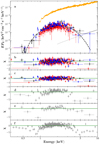 |
Fig. 5. Spectral energy distribution of 4U 0115+63. Panel (a): Unfolded EFE spectra during XMM-Newton observations Obs1 (black), Obs2 (blue), and Obs2016 (red) and fitted jointly. The dashed black curve represents the bbodyrad component. The dotted gray line shows a possible additional hard component, and the solid gray line indicates the total model spectrum. As a comparison, the spectrum of Obs3 is also in orange, and its low-energy part (< 1 keV) is excluded to simplify the panel. Residuals from the spectral fits using the bbodyrad and the bbodyrad + gaussian models are shown in panels (b) and (c), respectively. Panels (d), (e), and (f) show the residuals for Obs1, Obs2, and Obs2016, respectively, using the pegpwrlw model. |
At the same time, Wijnands & Degenaar (2016), Rouco Escorial et al. (2017, 2020) suggested that the spectra of 4U 0115+63 in quiescence can also be described by a power-law model with large photon index. We therefore attempted to replace the bbodyrad component with a pegpwrlw model in XSPEC. Consistent with Rouco Escorial et al. (2020), the model reveals a soft spectrum with the photon index Γ = 2.7 ± 0.2,  , and 2.7 ± 0.1 for Obs1, Obs2 and Obs2016, respectively. However, this model did not provide satisfactory fits to the spectra, yielding poor goodness-of-fit values: C-statistic/d.o.f. = 173.2/86 for Obs1, 55.4/37 for Obs2 and 464.4/202 for Obs2016. We show the residuals in Fig. 5. We also tested other models commonly used for accreting XRPs, such as comptt and cutoffpl, but the parameters could not be reliably constrained in either case due to the narrow energy band of XMM-Newton.
Similar to the timing analysis (e.g., the presence of red noise), the spectral shape of an XRP’s emission may provide strong evidence of either ongoing accretion or its absence. Notably, Tsygankov et al. (2019a) demonstrated that even at low mass accretion rates, the X-ray spectrum of XRPs cannot be adequately described by a simple blackbody model. In practice, at low luminosities (LX < 1035 erg s−1), XRP spectra typically exhibit a characteristic “two-hump” shape. This feature has been reported in several sources, including X Persei (Doroshenko et al. 2012), GX 304−1 (Tsygankov et al. 2019a), 1A 0535+262 (Tsygankov et al. 2019b), GRO J1008−57 (Lutovinov et al. 2021), and 2RXP J130159.6−635806 (Salganik et al. 2025). The hard spectral component is thought to arise partly from cyclotron radiation, originating from interaction of the accretion flow with the NS atmosphere, Comptonized in its upper hot layers (Nelson et al. 1995; Di Salvo et al. 1998; Coburn et al. 2001; Tsygankov et al. 2019b; Mushtukov et al. 2021; Sokolova-Lapa et al. 2021).
Mushtukov et al. (2021) and Sokolova-Lapa et al. (2021) modeled this scenario and successfully reproduced the overall shape of the low-luminosity spectra of A 0535+262 and GX 304−1. Both models predict that the position of the hard component coincides with the cyclotron energy of the pulsar. To test for the presence of a hard emission component related to the accretion process during the quiescent state, we added a gaussian component to our spectral model (i.e., const*tbabs*bbodyrad), fixing its central energy at 12 keV, corresponding to the fundamental cyclotron line of 4U 0115+63 (e.g., White et al. 1983). Following the suggestion by Tsygankov et al. (2019a) that the hard component typically contributes about half the flux of the soft component, we constrained the flux of the gaussian component in our fitting procedure to be half that of the blackbody component. However, the best-fit results gave a width of the gaussian close to zero. This suggests that the hard component is not necessary for the spectral fitting. We further fixed its width at 10 keV to enable a comparison between fits with and without the hard component, resulting a goodness-of-fit of C-statistic/d.o.f. = 392.2/325. The negative value of ΔC = −48.7 indicates that the two-component model provides a worse fit to the spectrum compared to the single-blackbody model. Therefore, the presence of a hard component in the quiescence spectrum can be tentatively ruled out. The corresponding fits are shown in Fig. 5. However, we note that the limited energy coverage of the available data restricts one to fully characterize the spectra above 10 keV, the spectral results should be interpreted with caution. Nevertheless, due to the low cyclotron line energy of 4U 0115+63, future broadband observations of this source would be valuable for understanding the radiation mechanisms in the low-luminosity state.
Using the single-blackbody model, we performed phase-resolved spectroscopy by dividing the pulse phase and corresponding spectra into four phase intervals (ϕ1 − 4 = 0 − 0.25, 0.25−0.5, 0.5−0.75, and 0.75−1), where phases are aligned with the pulse profiles shown in Fig. 4. The constant parameter was fixed to the values obtained from the phase-averaged spectra. The results are presented in Fig. 6 and Table 2. The blackbody temperature (kTBB) remains relatively stable across most of the spin phase but drops to 0.39 keV during the pulse trough. The blackbody radius exhibits a weak positive correlation with the pulse intensity, varying within the range RBB = 0.26 − 0.42 km. However, the low statistics of the phase-resolved spectra are insufficient for further investigating the dependence of flux on kTBB and/or RBB.
 |
Fig. 6. Phase-resolved spectral parameters of 4U 0115+63 obtained using the model const*tbabs*bbodyrad. Instrumental cross-calibration constants were fixed at their average values. Unabsorbed X-ray fluxes were calculated in the 0.5−10 keV energy range. The blackbody radius (RBB) is derived from the normalization of the bbodyrad component, assuming isotropic emission and a source distance of 5.0 kpc. The dotted gray lines in each panel indicate the average pulse profiles from Obs1, Obs2, and Obs2016 in arbitrary units. |
4. Discussion and conclusion
To investigate the origin of the X-ray emission from transient XRPs in the quiescent state, we conducted a timing and spectral analysis of the well-known BeXRP 4U 0115+63 using XMM-Newton observations obtained in 2023 following a type II outburst. As in previous post-outburst episodes observed in 2015 (Wijnands & Degenaar 2016; Tsygankov et al. 2016; Rouco Escorial et al. 2017) and 2017 (Rouco Escorial et al. 2020), the source displayed a low X-ray luminosity of ∼1033 erg s−1 during quiescence, along with type I outbursts occurring near periastron passages.
In systems where the accretion process occurs through the disk, as is expected in 4U 0115+63, the red noise arises from the stochastic nature of viscosity within the accretion disk (Lyubarskii 1997). Random fluctuations in viscosity lead to local variations in mass density, which propagate both inward and outward through the disk under the influence of viscous diffusion (Mushtukov et al. 2018, 2019). This process generates variability in the mass accretion rate at the inner disk radius, and the fluctuations are subsequently reflected at the NS surface, resulting in the observed variability of the X-ray flux (Revnivtsev et al. 2009). Viscous diffusion acts to suppress mass accretion rate fluctuations at frequencies higher than the local viscous frequency. However, even in a cold accretion disk (Tsygankov et al. 2017b) characterized by low viscosity, initial fluctuations are not entirely damped and can still propagate inward, reaching the inner disk radius and influencing the mass accretion rate onto the NS. In systems accreting from a stellar wind, variability in the mass accretion rate is instead driven by the intrinsic inhomogeneity, or clumpiness, of the wind (Walter & Zurita Heras 2007).
Timing analysis revealed the absence of low-frequency red noise in the PDSs of 4U 0115+63 during quiescence (Obs1, Obs2, and Obs2016). This contrasts sharply with Obs3, obtained near periastron passage, where a prominent red-noise component is detected in the PDS, consistent with the presence of accretion, as also indicated by the spectral analysis. As previously shown by Doroshenko et al. (2020), the lack of low-frequency variability is a characteristic feature of non-accreting systems, such as magnetars and radio pulsars.
The results of the joint spectral analysis of Obs1, Obs2, and Obs2016 suggest that the continuum emission of 4U 0115+63 during the quiescent state is well described by a single blackbody model, rather than the two-hump spectrum typically associated with low-level accretion in XRPs. This finding aligns with the timing analysis, which also supports a non-accreting scenario. We therefore conclude that, during these observations, the accreting material did not reach the NS surface due to the action of the centrifugal barrier, i.e., the propeller effect.
At the same time, X-ray pulsations at 0.277 Hz, corresponding to the NS spin frequency, are clearly detected in this regime in all three observations. The pulse profiles exhibit a sinusoidal-like shape accompanied by a weak harmonic component and a high root-mean-square pulsed fraction (PF > 50%), consistent with previous XMM-Newton observations (Rouco Escorial et al. 2017, 2020). This pulsation behavior has been interpreted as evidence of nonuniform thermal emission from the NS surface, likely caused by anisotropic cooling due to the presence of a strong magnetic field in the stellar crust (e.g., Geppert et al. 2006; Geppert & Viganò 2014). Pérez-Azorín et al. (2006) modeled the temperature distribution in the crust of a magnetized NS and found that the resulting X-ray spectrum can be well described by a single blackbody with an emitting area significantly smaller than the full stellar surface, consistent with our results. Depending on the crustal temperature distribution for different model configurations, the predicted pulsed fraction from this cooling scenario is in the range 15−28% for a NS with B ∼ 1012 G.
The tentative positive correlation between the blackbody temperature and the X-ray flux over the pulse phase (see the two upper panels in Fig. 6) further supports the interpretation of the emission as originating from a cooling atmosphere rather than from ongoing accretion. In a passively cooling, magnetized NS atmosphere, the temperature typically increases with optical depth (see, e.g., Shibanov et al. 1992), meaning that observers looking closer to the surface normal see deeper, hotter layers, while those viewing at larger angles sample cooler, upper layers. This geometry naturally leads to a positive correlation between the observed flux and blackbody temperature across the pulse phase. In contrast, accretion-heated atmospheres are expected to exhibit an inverse temperature profile, with external heating producing hotter upper layers (e.g., Suleimanov et al. 2018). In such a case, the observed flux could be anticorrelated with the apparent temperature, especially in the presence of significant optical depth effects. Therefore, the observed tentative temperature–flux correlation may serve as an indicator of anisotropic thermal cooling rather than ongoing accretion.
On longer timescales, we find that the observed quiescent flux decreased between 2016 and 2023 (see Tables 1 and 2). Such variability on year-long timescales cannot be explained by deep crustal heating, which evolves only over 104 − 105 yr (Brown et al. 1998). Instead, it points to processes operating in the outer crust. Similar conclusions were reached by Rouco Escorial et al. (2017, 2020), who studied the low-luminosity states of 4U 0115+63 after its 2015 and 2017 giant outbursts. In that case, the year-to-year differences in flux between post-outburst states can be naturally interpreted as changes in the amount of heat deposited during the preceding accretion episode.
Different authors, based on the magnetic hydrogen atmosphere models of a cooling NS, have theoretically predicted a spectrum similar to a blackbody (e.g., Zane et al. 2000; Ho & Lai 2001). We also modeled such emission using undisturbed magnetized hydrogen model atmospheres (Suleimanov et al. 2009). We computed a model atmosphere with parameters kTeff = 0.44 keV, M = 1.4 M⊙, R = 12 km, and a surface magnetic field normal to the atmosphere of 1.3 × 10¹² G. The emergent model spectrum is described well by a diluted blackbody with the flux of FE ≈ w π BE(fcTeff). A color correction factor of fc ≈ 1.25, and a dilution factor of w ≈ 0.41. This implies that the actual size of the emission region is larger than that inferred from a simple blackbody model, R ≈ w−1/2RBB ≈ 1.56 RBB.
We also investigated the angular dependence of the emergent model emission and find that radiation emitted tangentially to the surface, i.e., along the atmosphere plane, is less shifted to high energies (fc ≈ 1.1 for the zenith angle, θ, of 81°). It is interesting that the ratio of the observed blackbody temperatures of the pulse-average flux spectrum and the low-flux spectrum of the pulse profile is approximately equal to the ratio of the color correction factors for the flux spectrum and the intensity spectrum emitted at θ = 81°: 0.44 keV/0.39 keV ≈ 1.25/1.11 ≈ 1.13.
This means that the observed decrease in blackbody temperature can be explained by the model in which, at the pulse phase with the lower temperature, we see the bright spot inclined at a large angle to the line of sight. Thus, we conclude that a model of the magnetized NS atmosphere can explain the observed spectrum of the source and its phase dependence. More detailed modeling will be presented in a separate paper.
Future observational and theoretical studies of XRPs across different luminosity states will be valuable for advancing our understanding of emission mechanisms in highly magnetized NSs in quiescence. In particular, measurements of polarization properties could reveal the pulsar orientation (see, e.g., Poutanen et al. 2024) and help verify the models proposed above.
Acknowledgments
HX acknowledges support from the China Scholarship Council (CSC). AAM thanks UKRI Stephen Hawking fellowship. This research has made use of software provided by the High Energy Astrophysics Science Archive Research Center (HEASARC), which is a service of the Astrophysics Science Division at NASA/GSFC and the High Energy Astrophysics Division of the Smithsonian Astrophysical Observatory. This work is based on observations obtained with XMM-Newton, an ESA science mission with instruments and contributions directly funded by ESA Member States and NASA.
References
- Arnaud, K. A. 1996, ASP Conf. Ser., 101, 17 [Google Scholar]
- Brown, E. F., Bildsten, L., & Rutledge, R. E. 1998, ApJ, 504, L95 [NASA ADS] [CrossRef] [Google Scholar]
- Buccheri, R., Bennett, K., Bignami, G. F., et al. 1983, A&A, 128, 245 [NASA ADS] [Google Scholar]
- Campana, S., Gastaldello, F., Stella, L., et al. 2001, ApJ, 561, 924 [Google Scholar]
- Coburn, W., Heindl, W. A., Gruber, D. E., et al. 2001, ApJ, 552, 738 [NASA ADS] [CrossRef] [Google Scholar]
- Cominsky, L., Clark, G. W., Li, F., Mayer, W., & Rappaport, S. 1978, Nature, 273, 367 [NASA ADS] [CrossRef] [Google Scholar]
- Di Salvo, T., Burderi, L., Robba, N. R., & Guainazzi, M. 1998, ApJ, 509, 897 [NASA ADS] [CrossRef] [Google Scholar]
- Doroshenko, V., Santangelo, A., Kreykenbohm, I., & Doroshenko, R. 2012, A&A, 540, L1 [NASA ADS] [CrossRef] [EDP Sciences] [Google Scholar]
- Doroshenko, V., Santangelo, A., Suleimanov, V. F., & Tsygankov, S. S. 2020, A&A, 643, A173 [NASA ADS] [CrossRef] [EDP Sciences] [Google Scholar]
- Elsner, R. F., & Lamb, F. K. 1977, ApJ, 215, 897 [NASA ADS] [CrossRef] [Google Scholar]
- Geppert, U., & Viganò, D. 2014, MNRAS, 444, 3198 [Google Scholar]
- Geppert, U., Küker, M., & Page, D. 2006, A&A, 457, 937 [NASA ADS] [CrossRef] [EDP Sciences] [Google Scholar]
- Giacconi, R., Murray, S., Gursky, H., et al. 1972, ApJ, 178, 281 [NASA ADS] [CrossRef] [Google Scholar]
- Heindl, W. A., Coburn, W., Gruber, D. E., et al. 2000, AIP Conf. Ser., 510, 173 [Google Scholar]
- Ho, W. C. G., & Lai, D. 2001, MNRAS, 327, 1081 [Google Scholar]
- Huppenkothen, D., Bachetti, M., Stevens, A. L., et al. 2019, ApJ, 881, 39 [Google Scholar]
- Ikhsanov, N. R. 2001, A&A, 375, 944 [NASA ADS] [CrossRef] [EDP Sciences] [Google Scholar]
- Illarionov, A. F., & Sunyaev, R. A. 1975, A&A, 39, 185 [NASA ADS] [Google Scholar]
- Johns, M., Koski, A., Canizares, C., et al. 1978, IAU Circ., 3171, 1 [NASA ADS] [Google Scholar]
- Leahy, D. A., Darbro, W., Elsner, R. F., et al. 1983, ApJ, 266, 160 [NASA ADS] [CrossRef] [Google Scholar]
- Lii, P. S., Romanova, M. M., Ustyugova, G. V., Koldoba, A. V., & Lovelace, R. V. E. 2014, MNRAS, 441, 86 [Google Scholar]
- Lomb, N. R. 1976, Ap&SS, 39, 447 [Google Scholar]
- Lutovinov, A. A., Tsygankov, S. S., Karasev, D. I., Molkov, S. V., & Doroshenko, V. 2019, MNRAS, 485, 770 [NASA ADS] [CrossRef] [Google Scholar]
- Lutovinov, A., Tsygankov, S., Molkov, S., et al. 2021, ApJ, 912, 17 [Google Scholar]
- Lyubarskii, Y. E. 1997, MNRAS, 292, 679 [Google Scholar]
- Mukherjee, U., & Paul, B. 2005, A&A, 431, 667 [NASA ADS] [CrossRef] [EDP Sciences] [Google Scholar]
- Mushtukov, A., & Tsygankov, S. 2024, Handbook of X-ray and Gamma-ray Astrophysics (Singapore: Springer), 4105 [Google Scholar]
- Mushtukov, A. A., Ingram, A., & van der Klis, M. 2018, MNRAS, 474, 2259 [Google Scholar]
- Mushtukov, A. A., Lipunova, G. V., Ingram, A., et al. 2019, MNRAS, 486, 4061 [NASA ADS] [CrossRef] [Google Scholar]
- Mushtukov, A. A., Suleimanov, V. F., Tsygankov, S. S., & Portegies Zwart, S. 2021, MNRAS, 503, 5193 [Google Scholar]
- Nelson, R. W., Wang, J. C. L., Salpeter, E. E., & Wasserman, I. 1995, ApJ, 438, L99 [Google Scholar]
- Neumann, M., Avakyan, A., Doroshenko, V., & Santangelo, A. 2023, A&A, 677, A134 [NASA ADS] [CrossRef] [EDP Sciences] [Google Scholar]
- Orlandini, M., Bartolini, C., Campana, S., et al. 2004, Nucl. Phys. B Proc. Suppl., 132, 476 [Google Scholar]
- Pérez-Azorín, J. F., Miralles, J. A., & Pons, J. A. 2006, A&A, 451, 1009 [NASA ADS] [CrossRef] [EDP Sciences] [Google Scholar]
- Poutanen, J., Tsygankov, S. S., & Forsblom, S. V. 2024, Galaxies, 12, 46 [NASA ADS] [CrossRef] [Google Scholar]
- Raichur, H., & Paul, B. 2010, MNRAS, 406, 2663 [NASA ADS] [CrossRef] [Google Scholar]
- Rappaport, S., Clark, G. W., Cominsky, L., Joss, P. C., & Li, F. 1978, ApJ, 224, L1 [NASA ADS] [CrossRef] [Google Scholar]
- Reig, P. 2011, Ap&SS, 332, 1 [Google Scholar]
- Revnivtsev, M., Churazov, E., Postnov, K., & Tsygankov, S. 2009, A&A, 507, 1211 [CrossRef] [EDP Sciences] [Google Scholar]
- Rouco Escorial, A., Bak Nielsen, A. S., Wijnands, R., et al. 2017, MNRAS, 472, 1802 [NASA ADS] [CrossRef] [Google Scholar]
- Rouco Escorial, A., Wijnands, R., van den Eijnden, J., et al. 2020, A&A, 638, A152 [NASA ADS] [CrossRef] [EDP Sciences] [Google Scholar]
- Rutledge, R. E., Bildsten, L., Brown, E. F., et al. 2007, ApJ, 658, 514 [Google Scholar]
- Salganik, A., Tsygankov, S. S., Chernyakova, M., Malyshev, D., & Poutanen, J. 2025, A&A, 698, A71 [NASA ADS] [CrossRef] [EDP Sciences] [Google Scholar]
- Scargle, J. D. 1982, ApJ, 263, 835 [Google Scholar]
- Semena, A. N., Lutovinov, A. A., Mereminskiy, I. A., et al. 2019, MNRAS, 490, 3355 [Google Scholar]
- Shibanov, I. A., Zavlin, V. E., Pavlov, G. G., & Ventura, J. 1992, A&A, 266, 313 [NASA ADS] [Google Scholar]
- Sokolova-Lapa, E., Gornostaev, M., Wilms, J., et al. 2021, A&A, 651, A12 [NASA ADS] [CrossRef] [EDP Sciences] [Google Scholar]
- Stella, L., White, N. E., & Rosner, R. 1986, ApJ, 308, 669 [Google Scholar]
- Suleimanov, V., Potekhin, A. Y., & Werner, K. 2009, A&A, 500, 891 [NASA ADS] [CrossRef] [EDP Sciences] [Google Scholar]
- Suleimanov, V. F., Poutanen, J., & Werner, K. 2018, A&A, 619, A114 [NASA ADS] [CrossRef] [EDP Sciences] [Google Scholar]
- Tsygankov, S. S., Lutovinov, A. A., Doroshenko, V., et al. 2016, A&A, 593, A16 [NASA ADS] [CrossRef] [EDP Sciences] [Google Scholar]
- Tsygankov, S. S., Wijnands, R., Lutovinov, A. A., Degenaar, N., & Poutanen, J. 2017a, MNRAS, 470, 126 [Google Scholar]
- Tsygankov, S. S., Mushtukov, A. A., Suleimanov, V. F., et al. 2017b, A&A, 608, A17 [NASA ADS] [CrossRef] [EDP Sciences] [Google Scholar]
- Tsygankov, S. S., Rouco Escorial, A., Suleimanov, V. F., et al. 2019a, MNRAS, 483, L144 [NASA ADS] [CrossRef] [Google Scholar]
- Tsygankov, S. S., Doroshenko, V., Mushtukov, A. A., et al. 2019b, MNRAS, 487, L30 [NASA ADS] [CrossRef] [Google Scholar]
- Verner, D. A., Ferland, G. J., Korista, K. T., & Yakovlev, D. G. 1996, ApJ, 465, 487 [Google Scholar]
- Walter, R., & Zurita Heras, J. 2007, A&A, 476, 335 [NASA ADS] [CrossRef] [EDP Sciences] [Google Scholar]
- White, N. E., Swank, J. H., & Holt, S. S. 1983, ApJ, 270, 711 [NASA ADS] [CrossRef] [Google Scholar]
- Wijnands, R., & Degenaar, N. 2016, MNRAS, 463, L46 [NASA ADS] [CrossRef] [Google Scholar]
- Wilms, J., Allen, A., & McCray, R. 2000, ApJ, 542, 914 [Google Scholar]
- Zane, S., Turolla, R., & Treves, A. 2000, ApJ, 537, 387 [Google Scholar]
All Tables
Best-fitting spectral parameters for the averaged and phase-resolved spectra of 4U 0115+63.
All Figures
|
Fig. 1. Light curves of 4U 0115+63 during and after the 2023 giant outburst observed with Swift/BAT (gray) and XMM-Newton (red). The luminosities of XMM-Newton observations in the 0.3−10 keV band are |
| In the text | |
|
Fig. 2. Lomb-Scargle periodograms of 4U 0115+63 derived from three background-subtracted light curves with 0.1 s bins, observed by XMM-Newton in 2023. Clear pulsations are detected at a frequency of ≈0.277 Hz, corresponding to the NS spin frequency. |
| In the text | |
|
Fig. 3. PDSs of 4U 0115+63 normalized as in Leahy et al. (1983) and obtained using 0.1 s binned, background-subtracted light curves. The gray step line represents the PDS from Obs3, which clearly shows a red noise component at low frequencies. The red step line corresponds to the PDS from the combined light curves of Obs1, Obs2, and Obs2016, which exhibits a flat (white noise) distribution in the 0.003−1 Hz range. The inset provides a zoomed-in view around the NS spin frequency (highlighted by the green stripe). |
| In the text | |
|
Fig. 4. Pulse profiles from the XMM-Newton observations obtained during the quiescent (top) and accreting (bottom) states of 4U 0115+63, folded using background-subtracted light curves with 0.1 s binning in the 0.3−10 keV energy range and using spin periods estimated via epoch-folding. The profiles were normalized by their average count rates. Phases were aligned using the cross-correlation method. |
| In the text | |
|
Fig. 5. Spectral energy distribution of 4U 0115+63. Panel (a): Unfolded EFE spectra during XMM-Newton observations Obs1 (black), Obs2 (blue), and Obs2016 (red) and fitted jointly. The dashed black curve represents the bbodyrad component. The dotted gray line shows a possible additional hard component, and the solid gray line indicates the total model spectrum. As a comparison, the spectrum of Obs3 is also in orange, and its low-energy part (< 1 keV) is excluded to simplify the panel. Residuals from the spectral fits using the bbodyrad and the bbodyrad + gaussian models are shown in panels (b) and (c), respectively. Panels (d), (e), and (f) show the residuals for Obs1, Obs2, and Obs2016, respectively, using the pegpwrlw model. |
| In the text | |
|
Fig. 6. Phase-resolved spectral parameters of 4U 0115+63 obtained using the model const*tbabs*bbodyrad. Instrumental cross-calibration constants were fixed at their average values. Unabsorbed X-ray fluxes were calculated in the 0.5−10 keV energy range. The blackbody radius (RBB) is derived from the normalization of the bbodyrad component, assuming isotropic emission and a source distance of 5.0 kpc. The dotted gray lines in each panel indicate the average pulse profiles from Obs1, Obs2, and Obs2016 in arbitrary units. |
| In the text | |
Current usage metrics show cumulative count of Article Views (full-text article views including HTML views, PDF and ePub downloads, according to the available data) and Abstracts Views on Vision4Press platform.
Data correspond to usage on the plateform after 2015. The current usage metrics is available 48-96 hours after online publication and is updated daily on week days.
Initial download of the metrics may take a while.