| Issue |
A&A
Volume 702, October 2025
|
|
|---|---|---|
| Article Number | A136 | |
| Number of page(s) | 16 | |
| Section | Extragalactic astronomy | |
| DOI | https://doi.org/10.1051/0004-6361/202556569 | |
| Published online | 14 October 2025 | |
Deep imaging of the galaxy Malin 2 shows new faint structures and a candidate satellite dwarf galaxy
1
Instituto de Astrofísica de Canarias, Vía Láctea s/n, E-38205 La Laguna, Spain
2
Departamento de Astrofísica, Universidad de La Laguna, E-38206 La Laguna, Spain
3
Light Bridges S.L., Observatorio del Teide, Carretera del Observatorio s/n, E-38500 Guimar, Tenerife, Canarias, Spain
4
Université de Strasbourg, CNRS, Observatoire Astronomique de Strasbourg, UMR 7550, 67000 Strasbourg, France
⋆ Corresponding author: This email address is being protected from spambots. You need JavaScript enabled to view it.
Received:
23
July
2025
Accepted:
10
August
2025
Abstract
Giant low-surface-brightness (GLSB) galaxies represent an extreme class of disk galaxies characterized by exceptionally large sizes and low stellar densities. Their formation and evolutionary pathways remain poorly constrained, primarily due to the observational challenges associated with detecting their faint stellar disks. In this work, we present deep, multiband optical imaging of Malin 2, a prototypical GLSB galaxy, obtained with the newly commissioned Two-meter Twin Telescope (TTT) at the Teide Observatory. Our g-, r-, and i-band observations reach surface brightness depths of 30.3, 29.5, and 28.2 mag arcsec−2 (3σ, in areas equivalent to 10″ × 10″), respectively, enabling us to trace the stellar disk of Malin 2 out to a radius of ∼110 kpc for the first time. We observe new diffuse stellar structures, including a prominent stellar emission toward the northwest region of Malin 2. This emission coincides well with the H I gas distribution in this region. We also identify a faint spiral arm-like structure in the southeast of Malin 2. Additionally, we report the discovery of a very faint dwarf galaxy, TTT-d1 (μ0, g ∼ 26 mag arcsec−2), located at a projected distance of ∼130 kpc southeast of Malin 2. If physically associated with Malin 2, it would represent the first known satellite ultra-diffuse galaxy of a GLSB galaxy. We perform a multidirectional wedge photometric analysis of Malin 2 and find that the galaxy has significant azimuthal variations in its stellar emission. A comparison of the stellar mass surface density profiles of Malin 2 with those of a large sample of nearby spiral galaxies and other GLSB galaxies shows that Malin 2 lies at the extreme end of both these classes of objects in its radial extent and stellar mass surface density distribution. The spatial overlap between the asymmetric stellar emission and a lopsided H I distribution suggests that Malin 2’s GLSB disk has contributions from tidal interactions. Our results highlight the importance of ultradeep, wide-field imaging in understanding the structural complexity of GLSB galaxies. Upcoming surveys such as LSST will be crucial to determine whether the features we observe in Malin 2 are common to other GLSB disk galaxies.
Key words: galaxies: individual: Malin 2 / galaxies: star formation / galaxies: structure
© The Authors 2025
 Open Access article, published by EDP Sciences, under the terms of the Creative Commons Attribution License (https://creativecommons.org/licenses/by/4.0), which permits unrestricted use, distribution, and reproduction in any medium, provided the original work is properly cited.
This article is published in open access under the Subscribe to Open model. This email address is being protected from spambots. You need JavaScript enabled to view it. to support open access publication.
1. Introduction
Low-surface-brightness (LSB) galaxies are diffuse galaxies that are much fainter than the typical night sky surface brightness. The extreme faintness of LSB galaxies hinders in-depth observations even in the local Universe, and a large fraction of such galaxies are missing from most observations to date (Martin et al. 2019). In recent years, with the advent of powerful instruments, it has become possible to obtain deeper observations, allowing astronomers to study these galaxies with a new perspective.
Low-surface-brightness galaxies span a wide range of galaxy sizes, masses, and morphologies, from extreme size down to the more common dwarf galaxies. A giant LSB (GLSB) galaxy is an extreme type of LSB galaxy, with a huge LSB disk (scale length of 10 to 50 kpc; Sprayberry et al. 1995) and rich gas content (MHI > 1010 M⊙; Matthews et al. 2001). Sprayberry et al. (1995) classified GLSB disk galaxies using a diffuseness index criterion based on the B-band disk central surface brightness (μ0, B) and scale length (Rs). According to this definition, GLSB disk galaxies have a high diffuseness index, following the relation μ0, B + 5log(Rs) > 27, where μ0, B is mag arcsec−2 and Rs in kiloparsecs. The prototype of the class of GLSB galaxies is Malin 1, discovered by Bothun et al. (1987). The inner region of Malin 1 is an early-type high-surface-brightness spiral (SB0/a), surrounded by a huge LSB disk extending at least ∼120 kpc in radius, making it the largest spiral galaxy known (Moore & Parker 2006; Barth 2007). The origin of such GLSB galaxies is still debated, with several formation scenarios having been proposed (e.g., major mergers, high-spin dark matter (DM) haloes, low-density environments, satellite accretion, and head-on collisions; Saburova et al. 2021). The GLSB galaxies are thought to be rare due to their unusual disk extent and faintness. However, a recent work by Saburova et al. (2023) predicted that there could be about 13 000 GLSB galaxies just within z < 0.1. Until now, only 107 GLSB galaxies have ever been discovered (Zhu et al. 2023), indicating that a full census of these giants remains incomplete.
In this paper, we focus on Malin 2 (also known as F568-6), another prototypical GLSB galaxy similar to Malin 1. The morphological type of Malin 2 is that of a late-type (Scd) spiral with a huge extended disk (Kasparova et al. 2014). Sprayberry et al. (1995) classified Malin 2 as a GLSB disk with a B-band central disk surface brightness (μ0, B) of 23.4 mag arcsec−2 and a disk scale length (Rs) of 22.6 kpc. Malin 2 has an huge H I disk extending out to a radius of ∼120 kpc, rich in gas content with MHI ∼ 6 × 10¹⁰ M⊙, and a molecular gas fraction of up to 2% percent of the H I mass (Pickering et al. 1997; Das et al. 2010). Using long-slit spectroscopic observations and mass modeling, Kasparova et al. (2014) suggested that the giant disk of Malin 2 was likely formed due to a sparse and shallow DM halo, rather than any catastrophic scenarios such as major mergers. However, to rule out such scenarios, we also need deep imaging observations that can reveal the LSB signature of any past interactions, if any. In the case of Malin 1, deep imaging observations by Galaz et al. (2015) showed very LSB tidal features linking Malin 1 and a neighboring galaxy, indicating a likely past interaction between the two. However, in the case of Malin 2, it has never been imaged to sufficient surface brightness depths to trace such features. Existing optical data for Malin 2 such as the Sloan Digital Sky Survey (SDSS) and the Dark Energy Camera Legacy Survey (DECaLS) reach only down to a surface brightness depth of ∼28 mag arcsec−2 in the optical bands, leaving the outer regions of the stellar disk of Malin 2 largely unexplored.
In this work, we present the deepest optical imaging of Malin 2 to date, probing ∼2 mag arcsec−2 deeper than previous studies. We explore the previously unseen LSB stellar emission from the GLSB disk of Malin 2 to shed light on its true size and formation. Throughout this paper we adopt a flat ΛCDM cosmology with H0 = 70 km s−1 Mpc−1, ΩM = 0.27, and ΩΛ = 0.73. This corresponds to a projected angular scale of 0.904 kpc arcsec−1 for Malin 2 at a luminosity distance of 204.1 Mpc (z = 0.046).
The paper is structured as follows. Sect. 2 provides an overview of the data, observations, and reduction process. Section 3 focuses on the analysis and results. Sections 4 and 5 present the discussion and conclusions, respectively.
2. Data
We obtained the deep imaging of Malin 2 presented in this work using one of the newly commissioned Two-meter Twin Telescope (TTT), a Ritchey-Chrétien 2-m telescope located at Teide Observatory, Canary islands (Lat. 28° 18′04″ N, Long. 16° 30′38″ W). The camera used for the observations is a QHY600M Pro camera (sCMOS BSI detector) covering a field of view of 9.6′×6.5′ and a pixel scale of 0.06″ pix−1, although the data was re-binned in 3 × 3 pixels, resulting in a pixel scale of 0.194″ pix−1. As this is the first paper using the TTT data, in the following subsections we provide a detailed description of the observations and the data reduction.
We observed Malin 2 between March 25 and March 31, 2025, using g′-, r′-, and i′-band standard Sloan filters manufactured by Baader Planetarium (hereupon, we refer to them simply as g-, r-, and i-band filters). The total exposure times are 7.2 hours (g-band), 7.0 hours (r-band), and 3.2 hours (i-band), with a typical measured full width at half maximum (FWHM) in the images of 1.8″ for point-like sources and a typical sky brightness of 21.75, 20.75, and 20.35 mag arcsec−2 for g-, r-, and i-band filters, respectively.
The limiting 3σ surface brightness levels of our observations measured in regions equivalent to an area of 10″ × 10″ following Appendix A of Román et al. (2020) are 30.3 (g-band), 29.5 (r-band), and 28.2 (i-band) mag arcsec−2. Comparing these depths with the deep imaging surveys such as DECaLS DR10, we reach 1.5 magnitudes deeper in the g and r bands and 0.5 magnitude deeper in the i band in the Malin 2 field (DECaLS DR10, (3σ, 10″ × 10″)∼28.8, 28.1, and 27.7 mag arcsec−2).
2.1. Observational strategy
The strategy we used to gather the observations aimed to maximize the time spent observing Malin 2 and, at the same time, accurately characterize the illumination of the sky at the moment of the data collection. The sky characterization was fundamental in order to preserve the LSB structure and not introduce artificial structure in the images. Part of this sky characterization was done in the flat-field correction, and as is described in Sect. 2.2.1, we performed this correction using the scientific data itself, which allowed us to correct the inhomogeneous sensitivity of the detector (as a typical flat-field correction does), but without introducing the gradients present in the twilight or dome flats and correcting the illumination at the moment of the observations. However, in order to build this flat-field with the scientific exposures, we need a large-displacement dithering pattern (Trujillo & Fliri 2016). Thus, we built a dithering pattern with offsets of up to 6′, which is larger than the size of Malin 2 (∼4′), ensuring that there are exposures in which every pixel of the detector is free of sources and that we are always integrating on the galaxy. Additionally, due to the virtually nonexistent readout time (CMOS detector), we were able to efficiently do exposures of 1 minute, which contributed to minimizing saturation and getting a precise characterization of the sky.
2.2. Data reduction
We reduced the data using a pipeline specifically developed for preserving the LSB features of the data and minimizing the contamination present in the region of the observation (mainly gradients produced by the sky brightness). We describe the main steps of the data reduction process in the following subsections.
2.2.1. Bias, dark, and flat-field correction
The first step in the reduction of the data was to cope with saturated pixels and perform the bias correction. We solved the first of these tasks by masking all the pixels above 65 500 analog digital units (ADUs), which in the data are located at the central regions of some bright sources. We then applied the bias correction by subtracting a master bias (resulting from combining a set of individual biases) from the frames. Dark current is negligible in the detector for the exposure times we used, so we did not apply a correction to avoid introducing additional noise (Alarcon et al. 2023).
As is outlined in Sect. 2.1, we designed the observation strategy to allow performing the flat-field correction using science images, following a similar strategy to the one described in Trujillo et al. (2021) and Zaritsky et al. (2024). First, we normalized science images (bias-corrected) using the resistant mean of the values inside a ring that defines a constant-illumination section, centered on the center of the CCD, with an inner radius of 650 pixels and a width of 200 pixels. Then, we combined the normalized, bias-subtracted science images to build a flat. However, instead of using all the images to build a master flat, for each image, we used the ones that were close in time. This strategy allowed us to better characterize the sky illumination at the moment of the observation. The size of the window of frames used for this “running flat” strategy was 30 (i.e., we selected the 15 previous and following images).
We iterated this strategy for getting the flat-field three times to improve the quality of the results. On the first one, the flat was done by combining science images with a sigma clipping median stacking. On the second and third iterations, we first masked all the detected sources using Gnuastro1 NoiseChisel (Akhlaghi & Ichikawa 2015; Akhlaghi 2019), and then we median-combined the normalized, masked images. Each of these iterations produced a better flat field, allowing us to improve the quality of the data and build better masks, further improving the flat itself. Finally, we divided the individual science images by their corresponding flat. Additionally, to deal with vignetting problems toward the corner of the detectors, we removed all the pixels for which the masterflats had an illumination lower than 60% of the central pixels.
2.2.2. Astrometry
To determine the astrometry of the individual science images, we calculated a first astrometric solution using Astrometry.net (v0.94; Lang et al. 2010), with Gaia DR3 (Gaia Collaboration 2021) as our reference catalog. We then improved this first astrometric solution using SCAMP (v.2.10.0; Bertin 2006). SCAMP reads the catalogs generated by SExtractor (v2.25.0; Bertin & Arnouts 1996) to compute the distortion of the CCD. We repeated this process three times, as each iteration improves the previous solution. After that, we ran SWarp (v2.41.5; Bertin et al. 2002) to place the images into a common grid of 5250 × 5250 pixels, using the resampling method LANCZOS3.
2.2.3. Sky subtraction
Subtracting the sky is a crucial step that has to be tackled carefully in order not to introduce artificial structures or produce oversubtraction. We performed the sky subtraction individually on each frame, and, since the field of view of the data is not very large, we can work under the assumption of constant background. Additionally, not assuming any structure for the background rules out the possibility of introducing any artificial structure in the data.
To characterize the background, we built a mask that accounts for as much signal as possible. For this, we first built an aggressive mask using NoiseChisel and later we manually applied a mask centered on the galaxy with a radius of 120″. This mask over the galaxy was large enough that any region of undetected faint structure in its outskirts was not taken into account for the sky estimation. With the remaining unmasked pixels, we computed the sky value using a sigma clipping median and subtracted it from each of the frames.
2.2.4. Data combination
Once we had astrometrized the individual frames and subtracted their sky, they were ready to be combined. We combined the frames using a weighted mean, whereby each of the frames was weighed based on the standard deviation of its background. The reason behind this weighing scheme is that the quality of the frames varies between nights and even within one single night (e.g., illumination conditions, airmass, gradients related to the orientation of the observation), so this combination allows us to value more data of higher quality. Additionally, to perform an optimal combination, we applied the weights using a quadratic scheme, with the weight of the ith frame  , where σmin corresponds to the standard deviation of the less noisy frame.
The stacked image is deeper than the individual exposures, allowing faint structure that is below the noise in the individual images to now emerge. This previously undetected signal biased our estimation of the background (making us overestimate it), so we could now seize the information from the stacked image to define a more complete mask and apply it to the individual frames. With this improved mask, we calculated the background estimation again and went over all the subsequent steps described above, obtaining a final (non-calibrated) stacked image that is shown in Fig. 1.
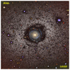 |
Fig. 1. Deep image of Malin 2 obtained from the TTT at Teide Observatory. The color composite image was created using g-, r-, and i-band filters with the Gnuastro package astscript-color-faint-gray (Infante-Sainz & Akhlaghi 2024). The black and white background corresponds to the g-band image. The image covers a field of view of 10′×10′ or 542.4 kpc × 542.4 kpc. North is up and west is right. |
2.2.5. Photometric calibration
The last step was to calibrate the stacked image. We converted pixel values from ADUs to physical units (Janskys) by matching the fluxes of stars in our image to the fluxes of stars in an already-calibrated survey. The survey used for the calibration is the Panoramic Survey Telescope and Rapid Response System (Pan-STARRS) DR1 (Chambers et al. 2016).
We downloaded the Pan-STARRS field of Malin 2 and generated a catalog of sources. We then matched this catalog with Gaia DR3 stars to obtain a clean sample of bona fide stars. Since we wanted to maximize the number of stars used for the calibration, instead of using just stars identified in Gaia, we looked at the range of FWHM that these stars had, using it as a criterion for selecting point-like sources in the Pan-STARRS images. Then we performed the photometry of the selected sources by using large enough apertures, which ensured that we virtually measured all the flux of the point-like source. If the aperture were too small, some flux would be lost in the tails of the PSF, generating inconsistencies when comparing fluxes measured on different images due to the differences in the PSFs. The use of a large number of stars effectively washes out the effect of the contaminants introduced by the large aperture. To define the aperture to use, we explored a wide range of apertures, studying the value at which the measured flux stabilizes. We concluded that for Pan-STARRS data, apertures of r = 9 Re are optimal. We then applied the same process to the data to calibrate, obtaining a catalog of point-like sources to be used for the calibration. The apertures used for measuring the flux are r = 7 Re. Additionally, to use non-saturated stars with a high signal-to-noise, for the calibration we used only sources with a magnitude between a certain range (15.5 < mag < 19.0, 15.0 < mag < 18.0, and 14.5 < mag < 17.0 for the g-, r-, and i-bands, respectively).
Since the photometric calibration is a complex task, surveys have non-negligible offsets between them. Thus, in order to be able to fairly compare data calibrated with different surveys, we decided to reference our calibration to an arbitrary but common framework, this being the Gaia spectra. This introduced a correction that we applied to the fluxes measured in Pan-STARRS, which were compared with the fluxes measured from the Gaia spectra and corrected (by applying an offset) to match them. Secondly, in order to give a precise photometry, we need to take into account the transmittance of the filters involved in the calibration. Even if technically we are working with the same filters (in this case g, r, i from Pan-STARRS and from TTT), there are differences in the filter response between the filters of different telescopes. This can be alleviated by applying a color correction. We characterized the applied color correction based on the g − r color and is determined using the Pan-STARRS filter shapes, the shapes of our filter, and GAIA spectra from stars in the field.
Finally, we matched the catalogs and calculated the factor that we needed to apply to our image in order to have it calibrated to physical units. The zero point was set to 22.5 in the AB magnitude system.
3. Analysis and results
3.1. Discovery of new LSB features in Malin 2
Our deep imaging of Malin 2 reveals, for the first time, several previously unseen LSB structures in the extended disk of the galaxy, which are shown in Fig. 1. In the northwest region, we detect a broad, diffuse stellar emission extending out to nearly 100 kpc from the galaxy center. This diffuse emission appears to align well with the outer H I contours from Pickering et al. (1997) (see Sect. 4.3 for more details). In the southeast of the galaxy, we see an elongated, spiral-arm-like structure emerging beyond the main optical disk, reaching surface brightness levels of μg ≈ 30 mag arcsec−2 at radii of ∼95 kpc. These features were barely detected and never reported in any of the previous imaging of Malin 2 (e.g., SDSS, DECaLS) due to the limited surface brightness sensitivity of these surveys. Fig. A.1 shows a comparison of the SDSS, DECaLS, and TTT imaging of Malin 2.
Our newly confirmed LSB structures show distinct morphological characteristics. The northwest diffuse emission exhibits a rather asymmetric structure with no clear spiral pattern, while the southeastern feature displays an arm-like morphology similar to an outer spiral structure or a tidal feature. These features demonstrate that Malin 2’s disk extends well beyond previous estimates and exhibits complex, non-axisymmetric structure in its outer regions.
Additionally, in the southeast region, at a projected distance of ∼130 kpc from the galaxy center, we identify a very diffuse source that appears to be a satellite galaxy of Malin 2 that is previously unknown. We provide a detailed photometric analysis of this source in Sect. 3.5.
3.2. Surface brightness profile measurements
The complex and asymmetric morphology of Malin 2, visible in our deep imaging, makes a traditional, azimuthally averaged surface brightness profile inadequate for characterizing its structure. Therefore, we performed a multidirectional radial profile measurement using wedge-shaped sectors to probe different galaxy orientations and quantify the structural asymmetries. We placed six wedges at angles of 0°, 60°, 120°, 180°, 240°, and 300° (measured counterclockwise from west toward north), each with an opening angle of 30° (see Fig. 2, left panel).
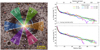 |
Fig. 2. Multidirectional photometry of Malin 2. Left: Wedge positions used for the photometry overplotted on the color image of Malin 2. Six wedges, each with 30° opening angles, are positioned at 0°, 60°, 120°, 180°, 240°, and 300°. A radial scale bar (in units of arcsec) is also shown along each wedge for easier comparison with the radial profiles. The location of the candidate dwarf satellite galaxy TTT-d1, discussed in Sect. 3.5, is marked in the bottom left corner (white circle). Right: Corresponding radial profiles of g- and r-band surface brightness for each wedge direction, showing significant structural asymmetry across different orientations. The dashed black line is the classical azimuthally averaged isophotal profile we measured, with the shaded gray region as its uncertainty. |
Before making radial profile measurements along the wedges, we created a mask to remove any background or foreground contaminants of the photometry. We created the mask using the MTObjects tool (Teeninga et al. 2016), on the combined g + r image. We ran MTObjects using a move_factor = 0.3, optimized for the detection of faint structures. We later visually inspected and manually edited the mask when necessary to ensure that all the contaminants were properly masked and none of the structures of Malin 2 were masked (e.g., spiral arms, diffuse regions). Hereupon, we use this mask throughout for our multiband photometry.
Within each wedge shown in the left panel of Fig. 2, we extracted surface brightness profiles with logarithmic radial bins ranging from the center of the galaxy to ∼125 kpc (140″) until we saw no visible signal in the optical images. We measured the local background sky level and noise at the last radial bin for each wedge separately. This was to take into account the local variations in the sky in addition to the global background subtraction we performed in Sect. 2.2.3. We truncated the radial profiles along each wedge at the radius where they reach the background noise. We performed the above wedge profile measurements for both the g- and r-band images. We did not attempt to do a similar procedure for our i-band data, as it is about 2 magnitudes shallower than our deepest g-band data (see Sect. 2). The i-band data in this work is used only to create the color images. From this point on, we corrected all the radial profiles for foreground Galactic extinction using the Schlegel et al. (1998) dust maps normalized by Schlafly & Finkbeiner (2011) and a Cardelli et al. (1989) dust extinction law. We also corrected all the profiles for inclination following Trujillo et al. (2020)2. For the inclination correction, we estimated the axis ratio of Malin 2 by running the AutoProf tool (Stone et al. 2021) on our g-band image, which is the deepest. We obtained an axis of b/a = 0.91 (inclination i = 23.9°) and a position angle (PA) of 72.7° corresponding to the 26 mag arcsec−2 isophote in the g band from the AutoProf fit. This value of inclination is about 14° lower than was previously reported for Malin 2, whereas the PA is highly consistent with the previous estimates (e.g., Pickering et al. 1997; Kasparova et al. 2014). However, since we have deeper imaging of Malin 2 in this work, we have chosen to adopt the values we estimated and we have corrected all our radial profiles for inclination throughout this work.
Figure 2 (right panel) presents the g- and r-band surface brightness profiles we measured for each wedge. The profiles reveal significant variations along different directions, with surface brightness differences of up to 2 mag arcsec−2 at large radii (R > 60 kpc) between different wedges. Most of the profiles reach down to a surface brightness level of ∼30 mag arcsec−2 and a radial extent of ∼110 kpc in both the bands. We verified that our profiles are consistent with the SDSS g- and r-band azimuthally averaged profiles from Kasparova et al. (2014). However, their profiles only reach a surface brightness level of 26 mag arcsec−2 (up to a 55 kpc radius), while ours extend about 4 magnitudes deeper and to twice the radial extent. The 240° and 300° wedges in our profiles show some early drop around 65 kpc compared to the other directions, as visible from the optical image. However, we see some additional stellar emission along these wedges at a radial range of 90 − 100 kpc, with a g-band surface brightness of ∼29 mag arcsec−2. This corresponds to the extended spiral-arm-like structure we observe in the south of the galaxy, which is discussed in Sect. 3.1. Similarly, along the 60° wedge, we see a clear excess in stellar emission within 80 − 100 kpc radius and a nearly constant g-band surface brightness of ∼28 mag arcsec−2. This corresponds to the diffuse stellar emission we see in the northeast part of the galaxy, as was mentioned in Sect. 3.1. The 180° wedge also shows a similar trend where we see an almost flat g-band surface brightness of ∼28 mag arcsec−2 within the radial range of 60 − 80 kpc, corresponding to the outer diffuse emission we see along this wedge in the left panel of Figure 2. Apart from the extended disk of the galaxy, in the inner regions (R < 60 kpc), the radial profiles along the different wedges seem to follow a similar trend on average, except for the visible local wiggles in the profiles that are likely due to the spiral arms (for instance, in the 300° wedge profile, we can clearly see a bump around 30 kpc that is due to the bright star-forming spiral arm visible in the optical image at this radius).
For a comparison to the wedge profiles, in Fig. 2, we also show the traditional azimuthally averaged surface brightness profiles of Malin 2. We obtained these average profiles by placing elliptical isophotes at a fixed PA and axis ratio (PA = 72.7°, b/a = 0.91) using the Isophote_Extract method of the AutoProf tool (Stone et al. 2021). The profiles were extracted using the same mask as was used for the wedge profiles. We measured the background estimate and noise along each isophote by placing 20 square boxes each of size 30″ at a distance of 140″ around the galaxy, following Gil de Paz & Madore (2005) and Junais et al. (2022). We can see that the average profiles shown in Fig. 2 agree well with the wedge profiles, but the directional asymmetries we see in the wedge profiles are mostly washed out, as was expected. This further illustrates the need for our wedge-based approach. Therefore, throughout this work, we focus more on the wedge profiles rather than the average profiles.
3.3. Color and stellar mass surface density profiles
Figure 3 shows the g − r color profiles (top panel) and the stellar mass surface density profiles (bottom panel) of Malin 2. We computed the stellar mass surface density profiles using Eq. (1) of Bakos et al. (2008), with a combination of the g − r color and g-band surface brightness profiles, following the color mass-to-light ratio relation from Roediger & Courteau (2015). Similar to the surface brightness profiles, both the color and stellar mass surface density profiles show diverse behavior in different directions. Colors vary from red to blue with g − r ∼ 1.2 mag in the center of the galaxy to ∼0.4 mag in the extended disk (in the case of the 240° and 300° wedges, g − r reaches up to ∼0.2 mag). Within the radial range of 20 kpc to 60 kpc, the color shows significant fluctuations along the different wedges due to the presence of several spiral arms. For instance, the 300° wedge profile shows a big drop toward a bluer color around 30 kpc radius as it passes through a bright spiral arm (similar to what we see in the surface brightness profiles and the optical image from Fig. 2). In contrast, the 180° wedge shows two red peaks around 30 kpc and 56 kpc radii, which also appear in the g − r color map shown in Fig. C.1, where we observe extended red emission along these radii. We confirm that these red peaks correspond to stellar populations in Malin 2 and are not due to any contamination from background emission.
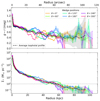 |
Fig. 3. Radial profiles of g − r color (top) and stellar mass surface density, Σ* (bottom), for each wedge direction in Malin 2. The horizontal dotted line in the bottom panel marks 1 M⊙ pc−2 stellar mass surface density, where we estimated the R1 radius in the manner discussed in Sect. 3.4. The colored legends for the wedge profiles are the same as in Fig. 2. The dashed black line is the classical azimuthally averaged isophotal profile we measure, while the shaded gray region is its uncertainty. |
Beyond the radius of 60 kpc, the 240° and 300° wedges show an early drop around 65 kpc, whereas the rest of the wedges extend well until a radius of ∼100 kpc (note that in the 240° and 300° wedges also we see some localized emission around 100 kpc, corresponding to the extended southeastern spiral-like structure we see in the optical images). In the extended disk of the galaxy (R > 60 kpc), the color profiles of all the wedges mostly stay flat around g − r = 0.4 mag, with a possible reddening beyond 90 kpc; however, with a large scatter. Apart from the one-dimensional radial color profiles shown in Fig. 3, the g − r color map shown in Appendix C shows the overall color distribution in Malin 2, both on and off the wedges we use in our measurements.
Figure 3 (bottom panel) shows the stellar mass surface density profile of Malin 2 along the wedges. It follows a rather smooth trend in all the wedges. The stellar mass surface density of the profiles reaches a peak value of ∼4 × 10⁴ M⊙ pc−2 in the center, with a steep decline within the 20 kpc by about 3 orders of magnitude, and reaches down to ∼0.1 M⊙ pc−2 at the outermost part of the disk around 100 kpc. All the wedges follow a similar trend up to 60 kpc radius (with minor differences corresponding to the spiral arms along the wedges). Similar to what we see in the color profiles, the stellar mass surface density profiles of the 240° and 300° wedges show a steep drop around 65 kpc radius. This is likely the optical edge of the galaxy at these azimuths, as we do not see any significant asymmetries along these two wedges. The remaining wedges all show a rather constant density value of ∼0.3 M⊙ pc−2 beyond this radius (see Table 1). Figure 3 thus shows that the outer diffuse asymmetrical structures we see in the optical images within the radial range of 60 to 100 kpc (beyond the main optical disk) have, on average, similar stellar density and colors, indicating a likely common origin for these structures.
Photometric properties of Malin 2 along different wedge directions.
3.4. Size estimates and stellar population properties of the extended disk
We measured the extent of the stellar disk in each wedge using the R1 radius, defined as the radius where the stellar mass surface density falls to 1 M⊙ pc−2 (Trujillo et al. 2020). Trujillo et al. (2020) chose that stellar mass surface density of 1 M⊙ pc−2 as it roughly corresponds to a proxy for the in situ star formation threshold in galaxies (e.g., Schaye 2004; Martínez-Lombilla et al. 2019). For galaxies with the stellar mass of the Milky Way, R1 is a good proxy for the location of the edge of the galaxy (Chamba et al. 2022). Recent works show that the R1 radius (a proxy for the edge) provides a physically motivated measure of galaxy size based on the end of the in situ star formation rather than the traditional scale length, effective radius, or R25 values (Trujillo et al. 2020; Chamba et al. 2020, 2022).
Table 1 shows our measured R1 radius for the different wedge profiles. We adopted the last radius at which the stellar mass surface density profiles that pass through the threshold of 1 M⊙ pc−2. For instance, the 60° wedge profile passes through the value of 1 M⊙ pc−2 twice, around 45 kpc and 63.3 kpc radii. We adopted the latter value. The R1 values range from a minimum of ∼53 kpc in the 0° wedge to ∼63 kpc in the 60° direction. The northern wedges (60° and 120°) show larger R1 values, above 60 kpc, consistent with the extended LSB features we detect in this region (see Fig. 2). All the other wedges have similar R1 values around 55 kpc. From all the wedge profiles, we get a mean R1 radius of 57.7 kpc for Malin 2. Note that the true extent of Malin 2 at lower surface brightness is even beyond this radius, as we can see from our profiles that it reaches up to a radius of about 110 kpc. On the other hand, it is worth noting that the R1 coincides pretty well with the location of the edge of the disk (i.e., where the mass profile drops in those wedges, unaffected by the tidal-like features).
We also estimated the effective radius (Re) of Malin 2 using the average isophotal g-band surface brightness profile shown in Fig. 2 (since by definition Re depends on the total light of the galaxy, it is only meaningful to use the average profile for the Re estimate than the wedge profiles). We estimated Re by non-parametrically integrating the average g-band profile to find the radius corresponding to the half of the total measured light. We obtained an Re of 20.3 kpc. This is about 2.8 times smaller than our mean R1 radius of 57.7 kpc. The mean R1 is also 2.5 times larger than the g-band disk scale length of 23.5 ± 4.5 kpc (26 ± 5 arcsec) reported by Kasparova et al. (2014) for Malin 2 from a bulge-disk decomposition of an azimuthally averaged profile. Due to the asymmetric nature of our profiles, in this work we have not attempted to perform a similar bulge-disk decomposition. A detailed comparison of our measured R1 radii with other spiral galaxies from the literature is given in Sect. 4.1.
Table 1 also shows our measured mean stellar properties of the extended disk of Malin 2 beyond a radius of 70 kpc. We adopted the value of R > 70 kpc to probe the diffuse stellar population visible in our imaging beyond the R1 radius. We verified that a choice of a different value (e.g., R > 60 kpc) for estimating the mean stellar properties in the outer disk does not make a significant change in the trends. All the wedges in this radial range, except the 300° wedge with a non-detection, show similar surface brightness level, color, and stellar mass surface density. The g-band surface brightness in these wedges (0°, 60°, 120°, 180°, and 240°) falls within a range of 28.3 to 29.2 mag arcsec−2 (a similar trend is seen in the r-band surface brightness levels too with a range of 27.8 to 28.8 mag arcsec−2). This gives a g − r color in the range of 0.39 to 0.51 mag and a stellar mass surface density of between 0.13 and 0.28 M⊙ pc−2. Therefore, the extended disk of Malin 2 has a mean g − r color of 0.44 mag and stellar mass surface density of 0.2 M⊙ pc−2. This indicates a relatively blue and young stellar population. Moreover, a rather similar stellar population across these multiple wedges points to a common origin for the diffuse emission in the extended disk of Malin 2. As an alternate approach to the wedge-based photometry, we also perform aperture photometry on several visually selected regions on the extended disk of Malin 2. We provide the results of these measurements in Appendix B. We find that they are consistent with our measurements from the wedge profiles.
3.5. Discovery of a diffuse galaxy: A likely new satellite of Malin 2
We identify a diffuse, LSB object that appears to be a satellite galaxy of Malin 2, in the southeast outskirts at a projected distance of 2.43′ (131.58 kpc at the distance of Malin 2) from the center of Malin 2, close to the edge of the 240° wedge in the left panel of Fig. 2. Here we report the discovery of this galaxy, clearly visible in our deep imaging, but barely visible in previous surveys (see Fig. 4). We name the dwarf galaxy TTT-d1 (the first dwarf galaxy discovered by the TTT telescope). TTT-d1 is located at coordinates of RA, Dec: 10h 39m 59.26s, +20d 48m 59.15s.
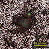 |
Fig. 4. Dwarf galaxy TTT-d1 discovered in the vicinity of Malin 2. The color composite image is created using g, r, and i-band filters with the Gnuastro package astscript-color-faint-gray (Infante-Sainz & Akhlaghi 2024). The black and white background corresponds to the g-band image. The image covers a field of view of 40″ × 40″ or 36.16 kpc × 36.16 kpc. |
To quantify the photometric and morphological properties of TTT-d1, initially we performed a GALFIT (Peng et al. 2010) Sérsic modeling of the g- and r-band images of the galaxy. We created the masks for the GALFIT modeling using the procedure discussed in Sect. 3.2. We present the results of our GALFIT Sérsic modeling in Table D.1. We find that TTT-d1 has a g-band effective radius of 6.38 ± 0.22″, Sérsic index (n) of 0.86 ± 0.03, and central surface brightness (μ0, g) of 25.94 ± 0.09 mag arcsec−2. We find similar quantities in the r band, with a slightly smaller effective radius (5.88 ± 0.23″). We obtain a mean g − r color of 0.53 ± 0.06 mag for TTT-d1, indicating a redder stellar population. We extracted azimuthally averaged radial surface brightness profiles for TTT-d1 in the g and r bands using the Photutils python package (Bradley et al. 2019). We used the same mask as in the previous step and followed the surface brightness profile measurement procedures from Junais et al. (2022). Figure D.1 shows our extracted profiles, overplotted with the best-fit GALFIT models obtained in the previous step. We can clearly see that the measured radial profiles of TTT-d1 are consistent with our independently estimated single Sérsic profiles.
Assuming the same distance of Malin 2, TTT-d1 has a g-band effective radius of 5.77 ± 0.20 kpc, central surface brightness of ∼26 mag arcsec−2, and stellar mass3 of 2.11 × 10⁸ M⊙. These properties are consistent with the known population of ultra-diffuse galaxies (UDGs) and demonstrate that such objects can exist as satellites in the halos of GLSB galaxies. With its large radial extend of ∼6 kpc, TTT-d1 will also be one of the largest known UDGs and comparable to the Nube galaxy from Montes et al. (2024). However, we should be cautious with such an inference, as we do not yet have an independent distance estimate for this source to confirm its association with Malin 2. While the large size of the TTT-d1 may reduce the likelihood of it being at the same distance as Malin 2, if confirmed, it could offer valuable constraints on the formation and evolution of GLSB galaxies. This will be done in future work.
4. Discussion
4.1. Comparison of Malin 2 to other spiral galaxies
To place Malin 2 in the context of the broader galaxy population, we compared its properties with a large sample of 273 spiral galaxies4 at z < 0.1 from Chamba et al. (2022). Figure 5 shows Malin 2’s position in the stellar mass versus R1 radius relation. With a stellar mass5 of log(M*/M⊙) = 11.3 ± 0.1 and a mean R1 radius of 57.7 ± 4.0 kpc, Malin 2 clearly stands out as one of the extreme cases, lying along the most massive and extended regime of spiral galaxies. This confirms Malin 2 as one of the most extended spiral galaxies known to date.
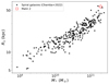 |
Fig. 5. Stellar mass versus R1 radius relation. Malin 2 (open red square) is compared to other spiral galaxies at z < 0.1 from Chamba et al. (2022) (black circles). Malin 2 clearly stands out as one of the extreme cases in this relation. |
The extreme size of Malin 2 can be visually illustrated by comparing it with scaled images of a few other spiral galaxies. Figure 6 (top panels) shows the image of Malin 2 compared to that of a spiral galaxy of similar stellar mass (J005042.73+002558.37; log(M*/M⊙) = 11.2) and a Milky Way-mass galaxy (J012015.34−002009.00; log(M*/M⊙) = 10.6), all scaled to the same physical dimensions in kpc. The Malin 2 image spans 271 kpc in width, whereas the other two images are 134 kpc and 69 kpc, respectively. We can see a significant difference in their radial extent. The Milky Way-mass galaxy (J012015.34−002009.00) appears significantly smaller in comparison. The stellar disk of Malin 2 extends far beyond that of J005042.73+002558.37, although both has almost the same stellar mass. Interestingly, J005042.73+002558.37 also has an R1 radius of 58.8 kpc, quite similar to Malin 2 (even slightly higher compared to the mean R1 of 57.7 kpc of Malin 2). This is the only galaxy in Fig. 5 that has a higher R1 than Malin 2. However, we can see that the radial extent of Malin 2 is well beyond the size of J005042.73+002558.37. This is expected as we see in the stellar mass surface density profile of Malin 2 from Fig. 3, the stellar emission of Malin 2 extends well beyond and to almost twice its R1. This also reinforces the idea that in both galaxies R1 is a good proxy for the end of the in situ star-forming disk, with one galaxy having no outer signatures of interactions (J005042.73+002558.37, J012015.34−002009.00) while the other (Malin 2) shows it.
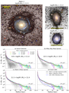 |
Fig. 6. Comparison of Malin 2 images and stellar mass surface density profiles with other spiral galaxies. Top: Visual size comparison showing Malin 2 (top left, log(M*/M⊙) = 11.3) compared to a spiral galaxy of a similar mass (J005042.73+002558.37; log(M*/M⊙) = 11.2 and a Milky Way-mass spiral (J012015.34−002009.00; log(M*/M⊙) = 10.6). All the images have the same physical scale. The images of the galaxies in the right column are retrieved from the IAC Stripe82 Legacy Project (Fliri & Trujillo 2016; Román & Trujillo 2018), which are about 1 magnitude shallower than our Malin 2 observations. Bottom: Stellar mass surface density profiles comparing Malin 2’s multidirectional wedge profiles (colored lines) with azimuthally averaged profiles of spiral galaxies from Chamba et al. (2022) (gray lines). The profiles are separated into four panels. Panel (a) is for all spirals, panel (b) Milky Way-mass spirals, and panel (c) Malin 2-mass spirals. All three panels are divided based on their stellar mass bins, as is shown in the label. Panel (d) compares Malin 2 with other GLSB galaxies; namely, Malin 1 (Boissier et al. 2016) and UGC 1382 (Chamba et al. 2022). The horizontal dash-dotted lines mark the 1 M⊙ pc−2 level. The azimuthally averaged isophotal profile of Malin 2 is shown as a dashed black line in all the panels. |
We provide a more quantitative comparison in the bottom panels of Fig. 6. We show the stellar mass surface density profiles of Malin 2 along different wedges obtained in Sect. 3.3 in comparison to the profiles of spiral galaxies from Chamba et al. (2022). The profiles are separated into different panels based on their stellar mass bins and types for a better illustration. Panel a of Fig. 6 shows the stellar mass surface density profiles of all the spiral galaxies from Chamba et al. (2022), whereas panel (b) compares only Milky Way-mass spirals and panel (c) spirals of a similar mass to Malin 2. Malin 2 stands out as an extreme case among all the galaxies shown and occupies the outermost envelope of the general profiles seen in other spiral galaxies (panel a of Fig. 6). This is a different illustration of the extreme nature we see in the visual comparison of Malin 2 with other spirals in the top panels of Fig. 6. Compared to both Milky Way-mass spirals and spirals with a similar mass to Malin 2, the stellar mass surface density profile of Malin 2 is extreme at all radii in its mass density and radial extent. In the case of panel c in Fig. 6, the early drops seen in the 240° and 330° wedges of Malin 2 are closer to the general trend observed in the profiles of other galaxies in that mass range. Nevertheless, even in those wedge profiles, Malin 2 is toward the extreme side. The remaining wedge profiles (0°, 60°, 120°, and 180°) do not show any similarity with any of the profiles from other spiral galaxies. This indicates that the faint extended stellar emission seen in the outer disk of Malin 2 (R > 70 kpc) is likely to have originated from some past interactions rather than a secular origin. However, it should be noted that the spiral sample does not have observations at the same depth as Malin 2 (about 1 magnitude shallower than our observations; Chamba et al. 2022). Due to this difference in depth, we cannot rule out the presence of faint, extended features in the spiral sample of Chamba et al. (2022) at lower surface brightness levels as we reach in Malin 2. However, we note that the large radial extent of Malin 2 is not a result of the deeper imaging we obtain in this work. For instance, Fig. E.1 shows a comparison of the stellar mass surface density profile of Malin 2 using DECaLS data and the profile we obtain in this work. We see that surveys such as DECaLS, which is comparable to the depth of the data used in Chamba et al. (2022), already show the large radial extent of Malin 2. However, the new faint features and asymmetric disk we see in this work are all almost invisible at the depth of those surveys.
4.2. Comparison to other GLSB galaxies
The GLSB galaxies in the literature are generally characterized by their ‘diffuseness index’ (di) based on the B-band disk scale length in kpc (Rs) and central surface brightness in mag arcsec−2 (μ0, B), where di = μ0, B + 5log(Rs) (Sprayberry et al. 1995; Hagen et al. 2016; Zhu et al. 2023; Bernaud et al. 2025). A galaxy with di > 27 is defined as a GLSB disk galaxy based on this diffuseness index criterion. Sprayberry et al. (1995) identified Malin 1, UGC 1382, UGC 6614, and Malin 2 as the most extreme cases of GLSB disks, with di values of 35.2, 32.7, 29.7, and 29.4, respectively. Among them, Malin 2 has the lowest di, indicating it is the least extreme case in comparison to Malin 1 or UGC 1382 based on their diffuseness index. However, this picture changes if we take a deeper look at panel d of Fig. 6, where we compare the stellar mass surface densities of Malin 2 with those of Malin 1 from Boissier et al. (2016) and UGC 1382 from Chamba et al. (2022). These two galaxies are the most extreme cases with the highest diffuseness index based on the Sprayberry et al. (1995) criterion. Based on panel d of Fig. 6, Malin 1 and UGC 1382 have a R1 radius of 26.5 kpc and 34.7 kpc, respectively. This is significantly smaller than the mean R1 that we obtain for Malin 2 (57.7 kpc), making Malin 2 the most extended among them based on the R1. Moreover, we should note that the diffuseness index criterion by Sprayberry et al. (1995) was formulated before the discovery of the extremely diffuse systems from current deep imaging surveys. Therefore, the diffuseness index criterion to select GLSB disk galaxies can also include some LSB dwarf galaxies such as UDGs. For instance, the satellite candidate galaxy TTT-d1 we identified in Sect. 3.5 also satisfies the diffuseness index criterion if we assume a disk morphology and the μ0, g and Re values from Table D.1. This suggests that the definition of GLSB galaxies based on the diffuseness index may benefit from an update. Perhaps incorporating radii such as R1 could lead to a more refined classification. However, this is beyond the scope of this work.
Malin 2 also shows interesting similarities (as well as some differences) to Malin 1 and UGC 1382 based on their stellar mass surface density profiles (see panel d of Fig. 6). The inner part of their profiles (R < 10 kpc) appears to follow a similar trend6. Between 10 < R < 60 kpc of their profiles, these three GLSB galaxies appear to be different. Malin 2 has a large amount of stellar mass distributed within this radial range, while Malin 1 has the lowest. Close to the radius of ∼65 kpc, the mass density profile of UGC 1382 appears to drop. This is quite similar to the drop in the 240° and 300° wedge profiles of Malin 2. Moreover, the UGC 1382 profile is well within the expected range found for other spiral galaxies, as we see in the previous panels of Fig. 6. Beyond the radius of 70 kpc (in panel d of Fig. 6), the stellar mass surface density profiles of both Malin 2 and Malin 1 look remarkably similar from 70 to 100 kpc in radial range, in terms of their slope and extent. Both these profiles show a significant flattening in this range, with an almost constant stellar mass surface density of ∼0.3 M⊙ pc−2. However, the flattening in the mass density profile of Malin 1 starts at a much smaller radius (∼30 kpc) compared to Malin 2 (which is only beyond 70 kpc). Junais et al. (2024) found that the flattening of the extended disk in Malin 1 agrees with the radial gas metallically profile from VLT/MUSE observations, which is almost constant at about 0.6 Z⊙ in the extended disk of Malin 1, indicating the enrichment from a past or ongoing interaction. The similarity of the stellar mass density profiles of both Malin 2 and Malin 1 in their extended disks could point toward a similar scenario for Malin 2 as well. However, we require more observations to confirm this (e.g., kinematics and metallicity from IFU observations), which is beyond the scope of this work.
4.3. Correlation of H I gas and stellar distribution: Implications for the formation of Malin 2
We compared our deep imaging of Malin 2 with the H I gas distribution from Pickering et al. (1997) to investigate the relationship between the stellar and gas components in Malin 2’s extended disk. Figure 7 shows the overlay of H I contours on our deep optical image. The H I distribution shows a clear asymmetry, with a significant elongation toward the northwest compared to a more truncated southeastern extent. Pickering et al. (1997) noted that the northwest H I extension in Malin 2 is about two times longer than that in the southwest, creating a significantly lopsided H I distribution (extending until 120 kpc). Interestingly, the newly detected northwestern stellar overdensity in our imaging shows clear spatial coincidence with this extended H I emission. Moreover, the H I emission extends slightly beyond our observed diffuse stellar emission in this region.
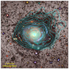 |
Fig. 7. Deep optical image of Malin 2 overlaid with H I column density contours from Pickering et al. (1997) (cyan lines). The H I contours are spaced linearly with ten contours ranging from a column density of 1.9 × 1019 cm−2 to the peak column density of 1.9 × 1020 cm−2. |
On the other hand, we do not see any H I emission associated with the stellar emission from the southeastern spiral-like structure or the dwarf galaxy (TTT-d1) visible in our imaging. Either these structures do not have any gas content within them, or they are too diffuse to be detected with the sensitivity of the VLA observations from Pickering et al. (1997). In the case of TTT-d1, with its mean g − r color of 0.53 mag (see Sect. 3.5), it is likely that gas content in this dwarf galaxy (if it exists) can only be detected at low H I column densities (NHI ∼ 1018 cm−2), as was recently found by the H I detection of LSB dwarf galaxies in the MONGHOOSE survey (Maccagni et al. 2024). Similarly, for the southeastern spiral-like structure, with its blue stellar population (see Tables 1 and B.1), the lack of detected H I emission might indicate a low-column-density gas (NHI < 1.9 × 1019 cm−2) below the sensitivity limits of the current VLA observations.
Jog & Combes (2009) suggested that lopsided H I distribution in galaxies is likely a result of tidal encounters, gas accretion, or a global gravitational instability. The elongated H I morphology to the northwest in Malin 2, together with the spatial overlap of the gas and stars in this region and the complex asymmetric stellar features revealed in our deep imaging, suggest that Malin 2’s extreme size and structure is likely a result of contributions from tidal processes rather than a pure secular evolution. Although Malin 2 is located in a relatively low-density environment, which is generally the case with GLSB galaxies (Saburova et al. 2021), we identified two galaxies (LEDA 1638675 and LEDA 1635102) that are at a comoving distance of about 0.6 Mpc and 2.4 Mpc from Malin 2, respectively. However, we do not see any additional evidence linking them in our optical imaging as well as the H I data. Additionally, there is also a galaxy group and cluster centered on the bright elliptical galaxies PGC 1645106 and PGC 032326, at a comoving distance of about 4 Mpc and 9 Mpc from Malin 2 toward the northeast direction, respectively. However, these distances are quite far for there to be any evident gravitational interactions. More follow-up observations are required to test if Malin 2 is undergoing any interactions or infalling toward these large scale structures.
5. Conclusions
We have presented deep, multiband optical imaging of Malin 2, a prototype of GLSB galaxies. We used data from the recently commissioned TTT at the Teide Observatory to reveal the complex structure of Malin 2 at unprecedented surface brightness levels. Our main results are as follows:
-
Our deep imaging reveals new stellar structures extending to ∼110 kpc, including a northwestern overdensity that correlates spatially with H I emission and a southeastern spiral-like extension reaching μg ≈ 30 mag arcsec−2.
-
We report the discovery of a dwarf galaxy (TTT-d1) in the vicinity of Malin 2, at a projected distance of about 130 kpc from its center. If confirmed to be at the distance of Malin 2, TTT-d1 will be the first satellite UDG around Malin 2.
-
A multidirectional wedge analysis of the surface photometry shows that Malin 2 has significant asymmetry in its stellar emission, color, and size in different directions. Such directional asymmetries would be missed by a traditional azimuthally averaged isophotal analysis.
-
By comparing Malin 2 to a large sample of nearby spiral galaxies and a few known GLSB galaxies, we find that Malin 2 lies at the extreme in its radial extent, which is larger and more extended than in any other nearby spiral or known GLSB galaxy.
-
The complex stellar features we identify in Malin 2, and their clear overlap with a lopsided H I gas distribution, suggest that Malin 2 experienced past interactions, which likely contributed to its GLSB disk formation.
Our findings highlight the importance of ultradeep, wide-field imaging for understanding the extreme population of GLSB galaxies. Recent deep imaging studies of other spiral galaxies have revealed complex substructures and satellite populations (e.g., Taibi et al. 2025). Our detection of a likely faint satellite around Malin 2 opens new avenues for constraining the formation histories of GLSB galaxies. Future observations from surveys such as LSST will allow for the analysis of larger samples of GLSB galaxies to determine whether the complex structures we observe in Malin 2 are typical of this population.
Data availability
The reduced images are available at the CDS via https://cdsarc.cds.unistra.fr/viz-bin/cat/J/A+A/702/A136
Acknowledgments
We are grateful to Timothy Pickering who kindly shared us with the processed Malin 2 H I data cube. We would like to acknowledge interactions with Mpati Ramatsoku, Mathias Urbano, Gauri Sharma and Pablo Manuel Sánchez-Alarcón. This article is based on observations made in the Two-meter Twin Telescope (TTT http://ttt.iac.es) sited at the Teide Observatory of the Instituto de Astrofísica de Canarias (IAC), that Light Bridges operates in Tenerife, Canary Islands (Spain). The Observing Time Rights (DTO) used for this research were consumed in the PEI “GALAXDIF25”. This research used storage and computing capacity in ASTRO POC’s EDGE computing center at Tenerife under the form of Indefeasible Computer Rights (ICR). The ICR were consumed in the PEI “GALAXDIF25” with the collaboration of Hewlett Packard Enterprise and VAST DATA. IT acknowledges support from the ACIISI, Consejería de Economía, Conocimiento y Empleo del Gobierno de Canarias and the European Regional Development Fund (ERDF) under a grant with reference PROID2021010044 and from the State Research Agency (AEI-MCINN) of the Spanish Ministry of Science and Innovation under the grant PID2022-140869NB-I00 and IAC project P/302302, financed by the Ministry of Science and Innovation, through the State Budget and by the Canary Islands Department of Economy, Knowledge, and Employment, through the Regional Budget of the Autonomous Community. This project is funded by the European Union (Widening Participation, ExGal-Twin, GA 101158446). J and JK acknowledge supplimentary funding from the European Union through the following grants: “UNDARK”, GA 101159929 and MSCA EDUCADO, GA 101119830. Views and opinions expressed are however those of the author(s) only and do not necessarily reflect those of the European Union or European Research Executive Agency (REA). Neither the European Union nor the granting authority can be held responsible for them.
References
- Akhlaghi, M. 2019, ASP Conf. Ser., 521, 299 [Google Scholar]
- Akhlaghi, M., & Ichikawa, T. 2015, ApJS, 220, 1 [Google Scholar]
- Alarcon, M. R., Licandro, J., Serra-Ricart, M., et al. 2023, PASP, 135, 055001 [NASA ADS] [CrossRef] [Google Scholar]
- Bakos, J., Trujillo, I., & Pohlen, M. 2008, ApJ, 683, L103 [NASA ADS] [CrossRef] [Google Scholar]
- Barth, A. J. 2007, AJ, 133, 1085 [NASA ADS] [CrossRef] [Google Scholar]
- Bernaud, E., Boissier, S., Junais, et al. 2025, A&A, 700, A56 [NASA ADS] [CrossRef] [EDP Sciences] [Google Scholar]
- Bertin, E. 2006, ASP Conf. Ser., 351, 112 [NASA ADS] [Google Scholar]
- Bertin, E., & Arnouts, S. 1996, A&AS, 117, 393 [NASA ADS] [CrossRef] [EDP Sciences] [Google Scholar]
- Bertin, E., Mellier, Y., Radovich, M., et al. 2002, ASP Conf. Ser., 281, 228 [Google Scholar]
- Boissier, S., Boselli, A., Ferrarese, L., et al. 2016, A&A, 593, A126 [NASA ADS] [CrossRef] [EDP Sciences] [Google Scholar]
- Bothun, G. D., Impey, C. D., Malin, D. F., & Mould, J. R. 1987, AJ, 94, 23 [NASA ADS] [CrossRef] [Google Scholar]
- Bradley, L., Sipocz, B., Robitaille, T., et al. 2019, https://doi.org/10.5281/zenodo.3478575 [Google Scholar]
- Cardelli, J. A., Clayton, G. C., & Mathis, J. S. 1989, ApJ, 345, 245 [Google Scholar]
- Chamba, N., Trujillo, I., & Knapen, J. H. 2020, A&A, 633, L3 [NASA ADS] [CrossRef] [EDP Sciences] [Google Scholar]
- Chamba, N., Trujillo, I., & Knapen, J. H. 2022, A&A, 667, A87 [NASA ADS] [CrossRef] [EDP Sciences] [Google Scholar]
- Chambers, K. C., Magnier, E. A., Metcalfe, N., et al. 2016, ArXiv e-prints [arXiv:1612.05560] [Google Scholar]
- Das, M., Boone, F., & Viallefond, F. 2010, A&A, 523, A63 [NASA ADS] [CrossRef] [EDP Sciences] [Google Scholar]
- Fliri, J., & Trujillo, I. 2016, MNRAS, 456, 1359 [Google Scholar]
- Gaia Collaboration (Brown, A. G. A., et al.) 2021, A&A, 649, A1 [NASA ADS] [CrossRef] [EDP Sciences] [Google Scholar]
- Galaz, G., Milovic, C., Suc, V., et al. 2015, ApJ, 815, L29 [NASA ADS] [CrossRef] [Google Scholar]
- Gil de Paz, A., & Madore, B. F. 2005, ApJS, 156, 345 [NASA ADS] [CrossRef] [Google Scholar]
- Hagen, L. M. Z., Seibert, M., Hagen, A., et al. 2016, ApJ, 826, 210 [NASA ADS] [CrossRef] [Google Scholar]
- Infante-Sainz, R., & Akhlaghi, M. 2024, Res. Notes Am. Astron. Soc., 8, 10 [Google Scholar]
- Jog, C. J., & Combes, F. 2009, Phys. Rep., 471, 75 [NASA ADS] [CrossRef] [Google Scholar]
- Junais, Boissier, S., Boselli, A., et al. 2022, A&A, 667, A76 [NASA ADS] [CrossRef] [EDP Sciences] [Google Scholar]
- Junais, Weilbacher, P. M., Epinat, B., et al. 2024, A&A, 681, A100 [NASA ADS] [CrossRef] [EDP Sciences] [Google Scholar]
- Kasparova, A. V., Saburova, A. S., Katkov, I. Y., Chilingarian, I. V., & Bizyaev, D. V. 2014, MNRAS, 437, 3072 [Google Scholar]
- Lang, D., Hogg, D. W., Mierle, K., Blanton, M., & Roweis, S. 2010, AJ, 139, 1782 [Google Scholar]
- Maccagni, F. M., de Blok, W. J. G., Mancera Piña, P. E., et al. 2024, A&A, 690, A69 [NASA ADS] [CrossRef] [EDP Sciences] [Google Scholar]
- Martin, G., Kaviraj, S., Laigle, C., et al. 2019, MNRAS, 485, 796 [NASA ADS] [CrossRef] [Google Scholar]
- Martínez-Lombilla, C., Trujillo, I., & Knapen, J. H. 2019, MNRAS, 483, 664 [CrossRef] [Google Scholar]
- Matthews, L. D., van Driel, W., & Monnier-Ragaigne, D. 2001, A&A, 365, 1 [NASA ADS] [CrossRef] [EDP Sciences] [Google Scholar]
- Montes, M., Trujillo, I., Karunakaran, A., et al. 2024, A&A, 681, A15 [NASA ADS] [CrossRef] [EDP Sciences] [Google Scholar]
- Moore, L., & Parker, Q. A. 2006, PASA, 23, 165 [NASA ADS] [CrossRef] [Google Scholar]
- Peng, C. Y., Ho, L. C., Impey, C. D., & Rix, H.-W. 2010, AJ, 139, 2097 [Google Scholar]
- Pickering, T. E., Impey, C. D., van Gorkom, J. H., & Bothun, G. D. 1997, AJ, 114, 1858 [NASA ADS] [CrossRef] [Google Scholar]
- Roediger, J. C., & Courteau, S. 2015, MNRAS, 452, 3209 [NASA ADS] [CrossRef] [Google Scholar]
- Román, J., & Trujillo, I. 2018, Res. Notes Am. Astron. Soc., 2, 144 [Google Scholar]
- Román, J., Trujillo, I., & Montes, M. 2020, A&A, 644, A42 [NASA ADS] [CrossRef] [EDP Sciences] [Google Scholar]
- Saburova, A. S., Chilingarian, I. V., Kasparova, A. V., et al. 2021, MNRAS, 503, 830 [NASA ADS] [CrossRef] [Google Scholar]
- Saburova, A. S., Chilingarian, I. V., Kulier, A., et al. 2023, MNRAS, 520, L85 [Google Scholar]
- Schaye, J. 2004, ApJ, 609, 667 [NASA ADS] [CrossRef] [Google Scholar]
- Schlafly, E. F., & Finkbeiner, D. P. 2011, ApJ, 737, 103 [Google Scholar]
- Schlegel, D. J., Finkbeiner, D. P., & Davis, M. 1998, ApJ, 500, 525 [Google Scholar]
- Sprayberry, D., Impey, C. D., Bothun, G. D., & Irwin, M. J. 1995, AJ, 109, 558 [NASA ADS] [CrossRef] [Google Scholar]
- Stone, C. J., Arora, N., Courteau, S., & Cuillandre, J.-C. 2021, MNRAS, 508, 1870 [NASA ADS] [CrossRef] [Google Scholar]
- Taibi, S., Pawlowski, M. S., Müller, O., et al. 2025, A&A, 699, A285 [NASA ADS] [CrossRef] [EDP Sciences] [Google Scholar]
- Teeninga, P., Moschini, U., Trager, S. C., & Wilkinson, M. H. F. 2016, Math. Morphol. Theory Appl., 1, 25 [Google Scholar]
- Trujillo, I., & Fliri, J. 2016, ApJ, 823, 123 [Google Scholar]
- Trujillo, I., Chamba, N., & Knapen, J. H. 2020, MNRAS, 493, 87 [NASA ADS] [CrossRef] [Google Scholar]
- Trujillo, I., D’Onofrio, M., Zaritsky, D., et al. 2021, A&A, 654, A40 [NASA ADS] [CrossRef] [EDP Sciences] [Google Scholar]
- Zaritsky, D., Golini, G., Donnerstein, R., et al. 2024, AJ, 168, 69 [Google Scholar]
- Zhu, Q., Pérez-Montaño, L. E., Rodriguez-Gomez, V., et al. 2023, MNRAS, 523, 3991 [NASA ADS] [CrossRef] [Google Scholar]
Appendix A: Comparison of archival data with our new imaging of Malin 2
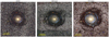 |
Fig. A.1. Comparison of Malin 2 images obtained from SDSS (left), DECaLS DR10 (middle) and the TTT at Teide Observatory (right). The color composite image is created using g, r and i-band filters with the Gnuastro package astscript-color-faint-gray (Infante-Sainz & Akhlaghi 2024). The black and white background corresponds to the g-band image. All the images are created using the same scale of contrast and zero point for a fair comparison. The images cover a field of view of 5′×5′. |
Appendix B: Aperture photometry of the diffuse regions in the extended disk
We perform aperture photometry measurements on several diffuse regions on the outermost part of the Malin 2 disk. Figure B.1 shows the regions that were visually selected based on the color image. We perform aperture photometry on these regions using the Photutils (Bradley et al. 2019) package and the same mask as used in Sect. 3.2. The background sky level and standard deviation for the measurements were estimated by placing a circular annulus of inner radius 130″ and width of 30″ around Malin 2, ensuring that it is outside the stellar emission from the galaxy. The results of the aperture photometry on these regions are given in Table B.1. Regions B and C have a similar g − r color with a mean value of 0.45 mag, corresponding to the northwest diffuse region from Sect. 3.1 and the 60° wedge from Sect. 3.2. Regions D and E have a bluer color than regions B and C, with a mean g − r of 0.23 mag. This indicates that the southeast spiral-arm-like structure seen in the optical image (corresponding to region E) has a young stellar population and is star-forming. Among all the 5 regions, Region A is the bluest. This is likely because a significant part of this region is an extension of the blue spiral arm visible in the optical image.
Aperture photometry results for diffuse substructures around Malin 2 as shown in Fig. B.1.
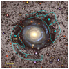 |
Fig. B.1. Color composite image of Malin 2 from TTT overlaid with visually identified regions of diffuse emission in the extended disk (cyan regions). See Table. B.1 for the photometric properties of each labeled region. |
Appendix C: Two-dimensional g − r color map of Malin 2
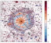 |
Fig. C.1. Two-dimensional g − r color map of Malin 2 obtained from the TTT data. The color map is smoothed by a Gaussian with sigma of 1 pixel (0.194″) for a better visualization of the LSB features. The black solid lines show the wedge positions used for the photometry in Sect. 3.2. Six wedges, each with 30° opening angles are positioned at 0°, 60°, 120°, 180°, 240°, and 300°. A radial scale bar (in units of arcsec) is also shown along each wedge for easier comparison with the radial profiles from Sect. 3.2. |
Appendix D: Photometry of the dwarf galaxy (TTT-d1) in the vicinity of Malin 2
Multiband Sérsic profile fitting results from GALFIT (Peng et al. 2010) for the dwarf galaxy (TTT-d1) near Malin 2.
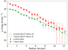 |
Fig. D.1. Radial surface brightness profiles of the dwarf galaxy (TTT-d1) near Malin 2. The g- and r-bands profiles are given in green circles and red squares, respectively. We measure the surface brightness profiles on elliptical isophotes using the Photutils python package (Bradley et al. 2019) and following the method from Junais et al. (2022). We fix the axis ratio and PA for the profile measurements to the g-band values from Table. D.1. The green dashed line and the red dot-dashed lines are the best fit Sérsic models (shown in Table. D.1) independently obtained from the 2-dimensional fitting of the g- and r-band images using GALFIT (Peng et al. 2010), respectively. The profiles shown here have not been corrected for inclination and foreground Galactic extinction. |
Appendix E: Stellar mass surface density profile comparison with TTT and DECaLS data
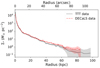 |
Fig. E.1. Comparison of the stellar mass surface density profiles of Malin 2 using the TTT data (black dashed line) and DECaLS data (red dash-dotted line). The shaded regions mark the 1σ uncertainty of the profiles. Both the profiles are measured following the same procedure as described in Sect. 3.3. We see that both the profiles agree well, but shows some differences beyond 40 kpc radius which are still consistent within a 3σ level of uncertainty. |
For the inclination correction, we assume a ratio of scale height to scale length of z0/h = 0.12 as given in Table 1 and Eq. (2) of Trujillo et al. (2020).
We estimate the stellar mass of TTT-d1 by converting the g- and r-band profiles to stellar mass surface density as described in Sect. 3.3. Assuming the distance of Malin 2, the stellar mass surface density profiles were integrated until the last measured radius to obtain the total stellar mass.
As the original sample of Chamba et al. (2022) also contains elliptical galaxies, here we include only the spiral galaxies with a TType ≥1 from their sample.
We estimate the stellar mass of Malin 2 by integrating the stellar mass surface density profiles shown in Fig. 3 for the different wedges. We use the mean stellar mass obtained from these multi-wedge profiles.
The Malin 1 stellar mass surface density profiles from Boissier et al. (2016), shown in Fig. 6, does not cover the very inner part of Malin 1 (R < 6 kpc) due to the low-resolution multiwavelength analysis performed in their work.
All Tables
Aperture photometry results for diffuse substructures around Malin 2 as shown in Fig. B.1.
Multiband Sérsic profile fitting results from GALFIT (Peng et al. 2010) for the dwarf galaxy (TTT-d1) near Malin 2.
All Figures
|
Fig. 1. Deep image of Malin 2 obtained from the TTT at Teide Observatory. The color composite image was created using g-, r-, and i-band filters with the Gnuastro package astscript-color-faint-gray (Infante-Sainz & Akhlaghi 2024). The black and white background corresponds to the g-band image. The image covers a field of view of 10′×10′ or 542.4 kpc × 542.4 kpc. North is up and west is right. |
| In the text | |
|
Fig. 2. Multidirectional photometry of Malin 2. Left: Wedge positions used for the photometry overplotted on the color image of Malin 2. Six wedges, each with 30° opening angles, are positioned at 0°, 60°, 120°, 180°, 240°, and 300°. A radial scale bar (in units of arcsec) is also shown along each wedge for easier comparison with the radial profiles. The location of the candidate dwarf satellite galaxy TTT-d1, discussed in Sect. 3.5, is marked in the bottom left corner (white circle). Right: Corresponding radial profiles of g- and r-band surface brightness for each wedge direction, showing significant structural asymmetry across different orientations. The dashed black line is the classical azimuthally averaged isophotal profile we measured, with the shaded gray region as its uncertainty. |
| In the text | |
|
Fig. 3. Radial profiles of g − r color (top) and stellar mass surface density, Σ* (bottom), for each wedge direction in Malin 2. The horizontal dotted line in the bottom panel marks 1 M⊙ pc−2 stellar mass surface density, where we estimated the R1 radius in the manner discussed in Sect. 3.4. The colored legends for the wedge profiles are the same as in Fig. 2. The dashed black line is the classical azimuthally averaged isophotal profile we measure, while the shaded gray region is its uncertainty. |
| In the text | |
|
Fig. 4. Dwarf galaxy TTT-d1 discovered in the vicinity of Malin 2. The color composite image is created using g, r, and i-band filters with the Gnuastro package astscript-color-faint-gray (Infante-Sainz & Akhlaghi 2024). The black and white background corresponds to the g-band image. The image covers a field of view of 40″ × 40″ or 36.16 kpc × 36.16 kpc. |
| In the text | |
|
Fig. 5. Stellar mass versus R1 radius relation. Malin 2 (open red square) is compared to other spiral galaxies at z < 0.1 from Chamba et al. (2022) (black circles). Malin 2 clearly stands out as one of the extreme cases in this relation. |
| In the text | |
|
Fig. 6. Comparison of Malin 2 images and stellar mass surface density profiles with other spiral galaxies. Top: Visual size comparison showing Malin 2 (top left, log(M*/M⊙) = 11.3) compared to a spiral galaxy of a similar mass (J005042.73+002558.37; log(M*/M⊙) = 11.2 and a Milky Way-mass spiral (J012015.34−002009.00; log(M*/M⊙) = 10.6). All the images have the same physical scale. The images of the galaxies in the right column are retrieved from the IAC Stripe82 Legacy Project (Fliri & Trujillo 2016; Román & Trujillo 2018), which are about 1 magnitude shallower than our Malin 2 observations. Bottom: Stellar mass surface density profiles comparing Malin 2’s multidirectional wedge profiles (colored lines) with azimuthally averaged profiles of spiral galaxies from Chamba et al. (2022) (gray lines). The profiles are separated into four panels. Panel (a) is for all spirals, panel (b) Milky Way-mass spirals, and panel (c) Malin 2-mass spirals. All three panels are divided based on their stellar mass bins, as is shown in the label. Panel (d) compares Malin 2 with other GLSB galaxies; namely, Malin 1 (Boissier et al. 2016) and UGC 1382 (Chamba et al. 2022). The horizontal dash-dotted lines mark the 1 M⊙ pc−2 level. The azimuthally averaged isophotal profile of Malin 2 is shown as a dashed black line in all the panels. |
| In the text | |
|
Fig. 7. Deep optical image of Malin 2 overlaid with H I column density contours from Pickering et al. (1997) (cyan lines). The H I contours are spaced linearly with ten contours ranging from a column density of 1.9 × 1019 cm−2 to the peak column density of 1.9 × 1020 cm−2. |
| In the text | |
|
Fig. A.1. Comparison of Malin 2 images obtained from SDSS (left), DECaLS DR10 (middle) and the TTT at Teide Observatory (right). The color composite image is created using g, r and i-band filters with the Gnuastro package astscript-color-faint-gray (Infante-Sainz & Akhlaghi 2024). The black and white background corresponds to the g-band image. All the images are created using the same scale of contrast and zero point for a fair comparison. The images cover a field of view of 5′×5′. |
| In the text | |
|
Fig. B.1. Color composite image of Malin 2 from TTT overlaid with visually identified regions of diffuse emission in the extended disk (cyan regions). See Table. B.1 for the photometric properties of each labeled region. |
| In the text | |
|
Fig. C.1. Two-dimensional g − r color map of Malin 2 obtained from the TTT data. The color map is smoothed by a Gaussian with sigma of 1 pixel (0.194″) for a better visualization of the LSB features. The black solid lines show the wedge positions used for the photometry in Sect. 3.2. Six wedges, each with 30° opening angles are positioned at 0°, 60°, 120°, 180°, 240°, and 300°. A radial scale bar (in units of arcsec) is also shown along each wedge for easier comparison with the radial profiles from Sect. 3.2. |
| In the text | |
|
Fig. D.1. Radial surface brightness profiles of the dwarf galaxy (TTT-d1) near Malin 2. The g- and r-bands profiles are given in green circles and red squares, respectively. We measure the surface brightness profiles on elliptical isophotes using the Photutils python package (Bradley et al. 2019) and following the method from Junais et al. (2022). We fix the axis ratio and PA for the profile measurements to the g-band values from Table. D.1. The green dashed line and the red dot-dashed lines are the best fit Sérsic models (shown in Table. D.1) independently obtained from the 2-dimensional fitting of the g- and r-band images using GALFIT (Peng et al. 2010), respectively. The profiles shown here have not been corrected for inclination and foreground Galactic extinction. |
| In the text | |
|
Fig. E.1. Comparison of the stellar mass surface density profiles of Malin 2 using the TTT data (black dashed line) and DECaLS data (red dash-dotted line). The shaded regions mark the 1σ uncertainty of the profiles. Both the profiles are measured following the same procedure as described in Sect. 3.3. We see that both the profiles agree well, but shows some differences beyond 40 kpc radius which are still consistent within a 3σ level of uncertainty. |
| In the text | |
Current usage metrics show cumulative count of Article Views (full-text article views including HTML views, PDF and ePub downloads, according to the available data) and Abstracts Views on Vision4Press platform.
Data correspond to usage on the plateform after 2015. The current usage metrics is available 48-96 hours after online publication and is updated daily on week days.
Initial download of the metrics may take a while.