| Issue |
A&A
Volume 703, November 2025
|
|
|---|---|---|
| Article Number | A277 | |
| Number of page(s) | 14 | |
| Section | Interstellar and circumstellar matterr | |
| DOI | https://doi.org/10.1051/0004-6361/202554149 | |
| Published online | 25 November 2025 | |
The accretion luminosity of Class I protostars
1
Alma Mater Studiorum - Università di Bologna, Dipartimento di Fisica e Astronomia “Augusto Righi”,
Via Gobetti 93/2,
40129
Bologna,
Italy
2
INAF-Osservatorio Astrofisico di Arcetri,
Largo E. Fermi 5,
50125
Firenze,
Italy
3
Astronomy & Astrophysics Section, School of Cosmic Physics, Dublin Institute for Advanced Studies,
31 Fitzwilliam Place,
Dublin
D02 XF86,
Ireland
4
European Southern Observatory,
Karl-Schwarzschild-Strasse 2,
85748
Garching bei München,
Germany
5
Institute for Astronomy, University of Hawaii,
Honolulu,
HI
96822,
USA
6
Université Paris-Saclay, Université Paris-Cité, CEA, CNRS, AIM,
91191
Gif-sur-Yvette,
France
7
Universität Heidelberg, Zentrum für Astronomie, Institut für Theoretische Astrophysik,
Albert-Ueberle-Str. 2,
69120
Heidelberg,
Germany
8
Universität Heidelberg, Interdisziplinäres Zentrum für Wissenschaftliches Rechnen,
Im Neuenheimer Feld 225,
69120
Heidelberg,
Germany
9
Harvard-Smithsonian Center for Astrophysics,
60 Garden Street,
Cambridge,
MA
02138,
USA
10
Elizabeth S. and Richard M. Cashin Fellow at the Radcliffe Institute for Advanced Studies at Harvard University,
10 Garden Street,
Cambridge,
MA
02138,
USA
11
INAF – Istituto di Astrofisica e Planetologia Spaziali,
Via Fosso del Cavaliere 100,
00133
Roma,
Italy
★ Corresponding author: leonardo.testi@unibo.it
Received:
15
February
2025
Accepted:
26
May
2025
Context. The value of the accretion luminosity during the early phases of star formation is crucial information that aids in understanding how stars form, but it is still very difficult to obtain.
Aims. We have developed a new methodology to measure accretion luminosity using mid-infrared hydrogen recombination lines and applied it to a limited sample of Class I protostars in the Taurus and Ophiuchus star-forming regions.
Methods. We adopted the commonly used assumption that the properties of disk-protostar accretion in Class I objects is similar to the disk-star accretion in Class II objects. Using simultaneous observations of three hydrogen recombination lines, Brγ, Pfγ, and Brα, we derived the mean intrinsic line ratios, and we verified that these are constant across the probed range of photospheric and accretion properties. We established correlations between the line luminosities and accretion luminosity.
Results. We measured the extinction toward the line emission regions in Class I protostars, comparing the observed line ratios to the Class II mean values. We then derived the Class I accretion luminosities from the established Class II correlations. We find that the accretion luminosity dominates the bolometric luminosity for the more embedded protostars, corresponding to lower values of the bolometric temperature. As the bolometric temperature increases above ~700 K, there is a sharp drop of the contribution of the accretion from the bolometric luminosity.
Conclusions. Our findings are in qualitative agreement with numerical simulations of star formation. We suggest our methodology be applied to larger and more statistically significant samples of Class I objects to obtain a more detailed comparison. Our results also suggest that by combining multiple infrared line ratios, it will be possible to derive a more detailed description of the dust extinction law in protostellar envelopes.
Key words: stars: formation / stars: pre-main sequence / stars: protostars / stars: variables: T Tauri, Herbig Ae/Be
© The Authors 2025
 Open Access article, published by EDP Sciences, under the terms of the Creative Commons Attribution License (https://creativecommons.org/licenses/by/4.0), which permits unrestricted use, distribution, and reproduction in any medium, provided the original work is properly cited.
This article is published in open access under the Subscribe to Open model. Subscribe to A&A to support open access publication.
1 Introduction
It is widely accepted that planets form in protoplanetary disks, which are the byproduct of the star formation process (Shu et al. 1987). The study of disks around pre-main sequence stars (so-called Class II disks; for the original definition of the young stellar objects classification scheme, see Lada 1987; Andre et al. 1993) has shown that in this phase, the disks are slowly evolving relics of more massive and dynamical structures that led to the rapid assembly of the central star and the formation of the planetary cores (e.g., Testi et al. 2022; Manara et al. 2023, and references therein). Though the Class II disks are important for understanding disk-planet interactions and the dissipation of disks, it is in the early phases (Class 0 and I) that planet formation most likely begins and most of the action takes place. Recent numerical simulations of star formation that include non-ideal magneto-hydrodynamics (MHD) and feedback effects and resolve the disk formation phase and extend up to the ages of the youngest Class I have shown that young star-disk systems are expected to have very high accretion luminosities that completely dominate the radiative output from the central object as well as the thermal structure of the young disks (Lee et al. 2021; Wurster 2021; Lebreuilly et al. 2024; Ahmad et al. 2025). Observationally, the disk-(proto)star interaction processes are still very poorly known in young embedded disks, yet they may play a critical role in shaping the overall initial conditions for planet formation (e.g., Hennebelle et al. 2020) and for the subsequent evolution of the star (e.g., Baraffe & Chabrier 2010). The lack of understanding is exemplified by the well-known “luminosity deficit” of protostars that seem to be under-luminous compared to the theoretically predicted accretion rates necessary to assemble the central protostellar mass within the duration of the embedded evolutionary phase (e.g., Kenyon & Hartmann 1990; Evans II et al. 2009). Several solutions for this conundrum have been proposed over the years, including a large spread of the accretion rates, both in time and environment conditions, leading to variable timescales to assemble the final stars (Fischer et al. 2023). These effects result in a large spread of accretion luminosities for protostars, as observed. As noted by Fischer et al. (2023), the observational characterization of the accretion luminosity in these early stages is still limited. In this context, it is essential to understand the contribution of accretion luminosities to the total bolometric luminosity of young disk-star systems. Numerical models predict that accretion dominates the total luminosity from the young disk-star system for a significant fraction of their early evolution, while measurements show that in the majority of cases, the observed accretion luminosity is less than 50% of the bolometric one (Fiorellino et al. 2023). As discussed by these authors, one of the most plausible reasons for this discrepancy is that the protostars for which the accretion luminosity could be reliably measured typically have a low extinction and are therefore representative of a late evolutionary stage.
The most successful methodology to accurately separate stellar and accretion luminosity contributions in young disk systems is based on the assumption that the observational accretion signatures (e.g., hydrogen emission lines) are related to the total accretion luminosity as in Class II objects so that the well-established Class II correlations between the emission line and accretion luminosities (e.g., Alcalá et al. 2017) can be applied to the earlier stages of evolution. Correlations between line luminosities and accretion luminosities have been established empirically, so lines can be used as a quantitative proxy of accretion, even if the line formation region is not necessarily confined to the accretion flow. For example, the recent optical interferometry study of GRAVITY Collaboration (2024) has found that the accreting material contributes only a small fraction of the total Brγ line flux in Herbig stars. In the case of young embedded disks, the detection of near-infrared lines (especially Brγ) is possible (e.g., Fiorellino et al. 2021; Antoniucci et al. 2011). The major limitation of these studies is the very uncertain extinction correction, which is also the reason for choosing low-extinction Class I objects as targets. More direct methods of measuring Lacc using the optical excess emission have been developed (White & Hillenbrand 2004), but again they are only applicable to a subset of objects with very low extinction and likely at the transition with the Class II stage.
Younger and more embedded protostars require a method for deriving an accurate measurement of the extinction, which can be computed from the observed line ratios if the intrinsic values are known. Beck (2007) attempted to use Brα and Brγ spectroscopy to derive extinction and accretion luminosity measurements for Class I objects in Taurus. The methodology for deriving extinction in that study relies on the assumption that the intrinsic line ratio follows the Case B theoretical ratio (e.g., Hummer & Storey 1987). In this paper, we propose a different approach based on the assumption that the intrinsic line ratio for Class I objects is the same as for Class II objects, which we derive empirically from observations. Thus, Lacc can then be computed from the extinction-corrected line luminosity using the correlations established for Class II objects, as in Fiorellino et al. (2021).
There is an obvious advantage to using hydrogen lines at longer wavelengths where the extinction is much smaller. The 4.05 µm Brα line is at least as strong as Brγ (Giovanardi et al. 1991) and much less affected by uncertainty in the extinction estimates. As an example, for a young disk with AV= 50 mag, the extinction at the Brγ wavelength is about 5 mag, while at the Brα wavelength, it is only ~2–3 mag (depending on the adopted extinction law Wang & Chen 2019, see also Sects. 4.1 and 6.1). However, this procedure requires characterization of the Class II hydrogen line spectrum in the mid-infrared to establish the values of the line ratios and the correlations of Lacc-Lline, which are currently unavailable, with very limited exceptions (Salyk et al. 2013; Rigliaco et al. 2015; Rogers et al. 2024b; Tofflemire et al. 2024). The purpose of this paper is to present a pilot study of what can be obtained from three hydrogen lines in the 2–4 µm region (Brγ (H(7-4), λ = 2.17 µm), Pfγ(H(8-5), λ = 3.74 µm), Brα(H5-4), λ = 4.05 µm). In this work, we first derive the mean values and their errors for two ratios (Pfγ/Brγ and Brα/Brγ) and then establish the relations between Lacc and L(Pfγ), and Lacc and L(Brα). Subsequently, we test how the Class II data can be used to derive the accretion luminosity in a sample of Class I objects and discuss the results.
We note that, more generally, this method can be used to derive the extinction correction for Class II objects located in very dense and obscured regions of their parental molecular cloud. For these objects more direct approaches (e.g., directly measuring the excess continuum luminosity at UV and optical wavelengths) cannot be applied, and extinction plays a dominant role in computing the correct line luminosities.
2 Observations and data reduction
The new spectra presented in this paper include eight Class II objects, seven T Tauri stars (TTSs) and one Herbig Ae star (HAE), and 17 Class I and flat spectrum objects located in the Taurus and ρ-Oph star-forming regions. The objects are listed in Tables 1 and 2, respectively.
The observations were performed using the SpeX instrument (Rayner et al. 2003, with the post 2014 upgrade) mounted on the NASA IRTF telescope. We used the LXD_short spectroscopic mode covering the wavelength range 1.67–4.2 µm and the 0.5 arcsec wide and 15 arcsec long slit, resulting in a spectral resolution of R~ 1500. Observations were carried out in four separate sessions on 19–20 July 2022, 26–27 April 2023, 23–24 November 2023, and 27 December 2023.
We adopted the standard SpeX observing strategy: nodding on slit for all point-like calibrators and targets; executing instrument calibration sessions every ~1.5 hours; integrating on target sources for 15–30 minutes, depending on the target brightness. Finally, we observed A0V bright stars at different air masses every night for telluric correction.
We followed the standard SpeX data reduction and spectral extraction procedures using the IDL software package spextool (Cushing et al. 2004). After calibration and combination of all the exposures for each target and telluric standard, we extracted and combined the spectra and used spextool to correct for telluric absorption. In order to check the final flux calibration, following the standard calibration steps, we imported the two spectral orders containing the Brγ line and the Brα and Pfγ lines in a custom Python procedure, and we compared our final spectra with 2MASS and Spitzer photometry. Typically, we found the discrepancy to be less than ~30%, and we decided to scale the spectra to match the photometry. Using this approach, we minimized the uncertainty on the relative calibration of the two bands. A possible continuum variability would result in a corresponding uncertainty in the estimated value of the accretion luminosity.
Line fluxes were computed fitting a Gaussian line profile to the spectra. The line fluxes measured for Class II objects are reported in Table 1, while those measured in Class I and flat spectrum sources are reported in Table 3. We do not explicitly include the possible uncertainty due to the flux calibration procedure discussed above.
Class II SpeX data.
Properties of the newly observed Class I/F and those from Beck (2007) (below the horizontal line).
3 Class II
As outlined in Sect. 1, we intended to use the line measurements on the Class II objects for two purposes. The first goal was to measure the fluxes of the ratios Pfγ/Brγ and Brα/Brγ and derive their mean values, which we used to infer the extinction in highly reddened objects. The second was to extend the correlation between optical and near-infrared lines and the accretion luminosity to lines at longer wavelengths.
Class I accretion properties.
3.1 Class II sample
To increase the number of stars and extend our sample toward objects of higher Lacc, we included the objects from Nisini et al. (1995), who observed the same infrared lines in a sample of intermediate-mass pre-main sequence stars. Our final Class II sample includes a few TTSs with a high Lacc and a number of HAeBe objects. This choice was motivated by the need to cover a line luminosity range comparable to what is expected for very young objects, such as Class I sources, which are known to have a higher Lacc than the older TTSs in well-studied nearby star-forming regions (Hartmann et al. 2016). We note, however, that this implies that the mass of the central stars in our Class I sample may differ from those in the Class II sample (the latter typically being of higher mass). This is probably not a problem, as the correlation between Lacc and the luminosity of individual hydrogen lines (Llines) does not significantly depend on the mass of the central star, with the possible exception of the very low mass stars and brown dwarfs (see Appendix B).
3.2 Class II line ratios
We proceeded by first deriving the intrinsic ratio of the Brα/Brγ and Pfγ/Brγ fluxes for the Class II objects observed with SpeX. We corrected the observed fluxes for extinction using the values tabulated in Table 1 and the Cardelli et al. (1989) extinction law with RV=3.1. For all stars in our sample, the observations of the three lines were either simultaneous (in the case of our SpeX observations) or executed within a few hours, such as in the case of the observations reported by Nisini et al. (1995). The total number of Class II objects is 25, and they all have detected Brγ lines. One has an upper limit in Brα, and two have upper limits in Pfγ.
The ratios of the dereddened fluxes are shown in Fig. 1. Each of the ratios cluster around a well-defined constant value independent of source properties, such as the stellar luminosity L★, accretion luminosity, and extinction (see Fig. 3). The mean value and its error are respectively Brα/Brγ=0.89±0.24 and Pfγ/Brγ=0.29±0.06. These values are briefly discussed in Sect. 7 in the general context of hydrogen line emission in Class II objects.
3.3 Class II Lacc-Lline relations
We derived the accretion luminosity, Lacc, of each object using the well-established existence of a correlation between Lacc and L(Brγ) (e.g., Muzerolle et al. 1998; Natta et al. 2006; Alcalá et al. 2017; Fairlamb et al. 2017), revised in Appendix B to include only objects with a high L(Brγ) and Lacc derived from UV excess emission:
 (1)
(1)
No similar datasets exist for Brα and Pfγ in the literature. For our sample, we do not directly have the values of Lacc computed from a measured UV excess. Therefore, we computed the correlations of these two lines with Lacc as derived from L(Brγ). In practice, we relied on the sample of Class II objects in Table 3. We computed Lacc from L(Brγ) and Eq. (1), and we derived the correlation between Lacc and L(Brα) (and L(Pfγ)). The uncertainties in the determination of the linear fit coefficients of Eqs. (2) and (3) were obtained by propagating the errors on the measured line fluxes and on the Lacc-L(Brγ) relation used to determine Lacc. The results are (see Fig. 2)
 (2)
(2)

Figure 3 shows the values of Lacc derived from L(Brα) (top panel) and L(Pfγ) (bottom panel) plotted as a function of the accretion luminosity derived from L(Brγ). The agreement between the values from L(Brα) and L(Pfγ) is very good and well within the uncertainties.
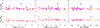 |
Fig. 1 Top panel: ratio of the de-reddened Brα and Brγ fluxes of Class II sources shown as a function of L★ (left), Lacc, computed from the Brγ luminosity (center; see Sect. 3.3), and the extinction in the K band (right). Bottom panel: same but for the ratio of Pfγ to Brγ fluxes. The values of the ratios are shown by filled dots; the 3σ upper limits are indicated by arrows. When not visible, the errors are smaller than the dots. In both sets of panels, the mean values of the ratios and their uncertainties are shown in orange. |
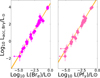 |
Fig. 2 Accretion luminosity, Lacc, derived from the Brγ luminosity (Eq. (1)) plotted as a function of the line luminosity for Brα (left panel) and Pfγ (right panel), respectively. The orange line and shadowed area show the best-fitting correlation and their uncertainty (see Eqs. (2) and (3)). |
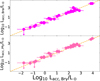 |
Fig. 3 Top panel: values of the accretion luminosity, Lacc, derived from L(Brα) as a function of Lacc derived from L(Brγ). Bottom panel: same but for Lacc derived from L(Pfγ). The line of equal values is shown in orange in each panel. |
4 Class I objects
In this section, we apply the results obtained for our Class II sample to derive the extinction toward each Class I object and then its accretion luminosity. Beck (2007) observed a sample of Class I sources in Taurus with the same instrument and setup we used. We include in our analysis the seven objects for which they detected Brγ and at least one among Pfγ and Brα. For homogeneity, we re-analyzed all of the objects using the same approach employed in our sample.
4.1 Extinction
The extinction in any of the three lines can be obtained from the ratio of two of them, once an extinction law is adopted. We computed the optical depth toward the Class I objects at the Brα wavelength from the observed flux ratio Robs=Brα/Brγ, assuming that the intrinsic ratio is the same as in Class II objects:
 (4)
(4)
The extinction is Aλ= 1.086 τλ. In Eq. (4), RII is the intrinsic Brα/Brγ extinction-corrected ratio for Class II objects (RII=0.89±0.24, see Sect. 3.2), and A2.17/A4.05 is the ratio of the extinction at the wavelength of the lines (Aλ = 1.086 × τλ). We adopted in all cases the extinction law WDOl with RV=5.5 (Weingartner & Draine 2001), as it is more suitable for the dense regions surrounding Class I sources (appropriate for AK ≥ 2.0, also according to Li & Chen 2023); the corresponding ratio is A4.05/A2.17 = 0.534. We proceeded in the same way to derive the optical depth at the Pfγ line from the observed Pfγ/Brγ flux ratio:
 (5)
(5)
where Robs=Pfγ/Brγ, RII=0.29±0.06 for Pfγ/Brγ (Sect. 3.2), and A3.74/A2.17 = 0.573.
The extinctions derived for Brα and Pfγ are given in Table 3. While the two extinctions were computed independently, we checked that the corresponding extinctions in K are equal within the uncertainty (see Fig. 4). The values of the extinction for the sources in our sample are in the range of AK~1–8 mag (AV~ 10–80 mag).
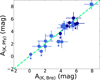 |
Fig. 4 Accretion luminosity computed from Pfγ shown as a function of the accretion luminosity computed from Brα for Class I objects. In the first case, the extinction is derived from the ratio Pfγ/Brγ, and in the second it is from Brα/Brγ (see Sect. 4.1). Dark blue dots are objects in Ophiuchus; light blue dots are objects in Taurus. Light blue squares are Taurus objects from Beck (2007). The green dashed line shows the locus of equal values. |
4.2 Accretion luminosity
The accretion luminosity of each object was computed from the luminosity of Brα and Pfγ corrected for extinction and as derived in the previous section using the correlation between the line luminosity and Lacc derived in Sect. 3.3. The two values agree well within uncertainties, as shown in Fig. 5. We note that the errors include the contributions from the observed line fluxes, the extinction at the wavelength of the line we used to measure Lacc, and the uncertainty on the relation Lacc-L(Brα) (or Lacc-L(Pfγ)). The values displayed in Table 3 are derived from the Brα line, as this line is detected in all objects and the values of Lacc derived from it are more accurate than the value derived from the other two lines. These Lacc values are the ones we use in the rest of the paper, and we refer to them as Lacc for simplicity.
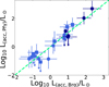 |
Fig. 5 Extinction in the K band computed from the ratio Pfγ/Brγ is shown versus the value derived from the Brα/Brγ ratio (see Sect. 4.1). Symbols are as in Fig. 4. The green dashed line shows the locus of equal values. |
4.3 Foreground extinction, bolometric luminosity, and temperature
To compute the bolometric luminosities (Lbol) and bolometric temperatures (Tbol) of all of our sources, we followed the general methodology of Dunham et al. (2015) but with the important difference that we tried to evaluate the foreground extinction for each of our sources independently (instead of using full cloud averages). For each target, we selected an area with a radius of 150″, or about 0.1 pc at the distance of our targets, and we computed the average extinction of all Class II within this area (from the catalogs of Esplin & Luhman 2019; Esplin & Luhman 2020, for Taurus and Ophiuchus, respectively). The choice of the maximum separation was based on ensuring that a few Class II stars are available to compute an average extinction for each Class I object. Two of our objects (SSTc2d J163135.6–240129 and SSTc2d J163200.9–245642) are outside the area surveyed by Esplin & Luhman (2020), and for these we adopted the average cloud extinction value of Dunham et al. (2015).
We decided to use the average foreground extinction using Class II stars within ~0.1 pc around each of our targets, instead of the average cloud extinction, because we noticed that Class II sources located in the vicinity of our targets show a significantly higher extinction than average. This is not surprising, as Class I sources are typically found in the denser regions of molecular clouds, while the full Class II population is much more dispersed (Evans II et al. 2009), leading to lower average foreground extinction. The average uncertainty of our computation of the foreground extinction is about ΔAK ~ 1 mag. The derived values of AK,fg, Lbol, and Tbol are listed in Table 2. Compared to the estimates of Dunham et al. (2015), our values of Lbol and Tbol are generally higher, by up to a factor of about two, for objects with the largest values of AK,fg. In the range of AK,fg of our sample (~0.5–3.2), we found no correlation between the foreground extinction and the derived Lbol and Tbol, as expected.
The uncertainty in AK,fg has a small impact on the derived values of Lbol and Tbol for sources with large values of AK,fg and small values of Tbol, while the effect is much larger for sources with high values of Tbol (see Fig. 6). This is not surprising, as sources with a high Tbol have significant emission at short wavelengths, where an uncertain extinction correction will produce the largest variations. This implies that our computed values of Lbol and Tbol for the youngest sources are less affected by the uncertainty in the estimate of AK,fg For high Tbol sources, which are mostly part of the Taurus sample, our error bars are generally consistent with these objects being more evolved (possibly Class II objects previously misclassifled as Class I or F).
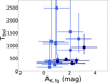 |
Fig. 6 Bolometric temperature plotted against the computed foreground extinction (AK,fg). Symbols are as in Fig. 4. |
5 Discussion
5.1 Evolution of the Lacc/Lbol ratio
The values of Lacc derived in the previous section span a range from ≲1 to ~100 L⊙ (see Fig. 7). In all but one of the objects with Tbol ≤ 500 K, within the uncertainties, Lacc is comparable to the total bolometric luminosity, as shown in Fig. 8, where the ratio Lacc/Lbol is plotted as a function of the bolometric temperature Tbol. Also, all but one of the objects with Tbol ≥ 800 K are compatible with Lacc being a small fraction of Lbol (even though the uncertainties in the Lbol measurements are very large for this subsample, as noted above). Only one of the low accretors in Taurus has Tbol ≤ 500 K, and one high accretor in Ophiuchus has Tbol ~1000 K. We note that in some cases the derived Lacc/Lbol ratio is larger than one. This can be due to different reasons, such as the variability of Lacc or Lbol (see below), or related to the source geometry (see Sect. 6.2).
It is generally expected that younger objects, where a high fraction of the luminosity is due to accretion, are also more embedded in the parental core and therefore have a higher extinction due to local dust (e.g., Evans II et al. 2009). We computed the local extinction, Alocal, as the difference between the total extinction derived from the line ratios (see Table 3), which depends on the total amount of dust along the line of sight, and the foreground component, Afg. Figure 9 shows the results for the K band. Most low accretors have a low local extinction, AK,local ≲ 1 mag, while most of the high accretors have AK,local ≳ 2 mag. In spite of the large uncertainties that affect some of the results, the transition between high to low accretors at Tbol is ~500–700K. This trend is broadly consistent with the expectations from numerical models of star formation. For example, one result of Lebreuilly et al. (2024) is that proto-stars have an initial evolutionary phase in which Lacc dominates the instantaneous total luminosity of the central protostar. Then there is a sharp transition to the total luminosity being dominated by the internal luminosity of the central source. We note that one important difference between the “total” luminosity computed in the models and the “bolometric” luminosity derived from observations is related to the temporal averaging introduced by the reprocessing of radiation in the protostellar envelope. While in observations it is possible to have occurrences of the instantaneous Lacc being larger than the Lbol, in models the instantaneous total luminosity of the central source is always the sum of the instantaneous accretion and internal luminosities.
The fact that in most of the Ophiuchus Class I sample the accretion luminosity accounts for all of the Lbol while Taurus objects cover a large range of values, from accretion to stellar-dominated luminosity, is likely a selection effect. Indeed, the Ophiuchus Class I sample contains objects selected because of their low values of Tbol already corrected for an estimated average foreground extinction (Dunham et al. 2015), while the selection of Taurus Class I objects had less stringent criteria. The objects classified as Class I purely on the basis of their observed infrared spectral index (uncorrected for foreground extinction) may in fact cover quite a significant range of different evolutionary stages, such as from a time when the central star is still significantly growing to a later phase where the central object has already reached a mass close to the final one, and the photospheric luminosity controls the thermal structure of the surroundings.
This picture is in agreement with other studies of accretion in young stellar objects. Fiorellino et al. (2023) show that in Class I sources Lacc≲ 0.5 Lbol in a sample selected for low values of extinction, which is consistent with relatively evolved Class I young stellar objects. In their sample, ~80% of the sources show AK≤ 3, whereas in our sample (see Fig. 9), ~80% of the sources with AK ≤3 show Tbol≥700 K. Le Gouellec et al. (2024) observed Brγ line luminosities for a sample of face-on, hence low-extinction, younger Class 0 young stellar objects. They show that at younger ages, the line luminosity is a factor of ~100 higher than in the sample of Fiorellino et al. (2023).
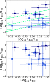 |
Fig. 7 Accretion luminosity (top) and fraction of accretion luminosity over bolometric luminosity (bottom) as a function of Lbol. Symbols are as in Fig. 4. The green dotted lines show the locus of Lacc/Lbol=l, 0.1, and 0.01, as marked. |
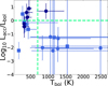 |
Fig. 8 Ratio of the accretion luminosity to the bolometric luminosity as a function of Tbol. Symbols are as in Fig. 4. The dotted green lines show the Tbol=700 K and the Lacc=Lbol locus. |
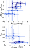 |
Fig. 9 Top panel: ratio of Lacc/Lbol versus the local extinction in the K band AK,local. Bottom panel: Tbol versus AK,local. Symbols are as in Fig. 4. |
5.2 Comparison with numerical simulations
Numerical simulations of star formation have now reached a level of sophistication that allows us to estimate the variation of Lacc as the objects evolve in time. To produce a qualitative comparison with our results, we used the Lacc, Ltot, age, and mass of the protostars for a fully consistent population formed within a single numerically simulated star-forming cloud in the high resolution non-ideal MHD simulations of Lebreuilly et al. (2024). We note that for this analysis, the Ltot values were computed as the sum of the accretion and intrinsic luminosities of the growing sink particles, which represent the (proto-)stars in the simulation. The value of Ltot is thus the total luminosity of the compact protostar, which may differ from the observed Lbol, as the latter is derived from the line of sight’s reprocessed radiation through the envelope (see Sect. 6).
In Figure 10, we show the values of the ratio Lacc over Ltot as predicted by the numerical simulations of Lebreuilly et al. (2024). The simulations show that Lacc dominates Ltot at early stages of evolution, and then the contribution of the accretion to the total luminosity drops very rapidly at later evolutionary stages. In the simulations, the transition occurs when the central protostar reaches a critical internal luminosity threshold.
The same qualitative behavior is obtained in simulations with different assumptions on the underlying physics Lebreuilly et al. (2024 e.g., with mechanical feedback or low magnetization). A more detailed comparison of our measurements with the outcome of currently available numerical simulations remains difficult because of the mismatch in the ages of the objects.
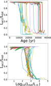 |
Fig. 10 Ratio of Lacc/Ltot versus age (top) and Ltot (bottom) from the simulations of Lebreuilly et al. (2024). |
6 Caveats
6.1 Extinction correction
The results discussed above depend significantly on the adopted extinction law in the region ~2–1µm. There is a large uncertainty on what is the most appropriate extinction law for the dense cores of Class I objects. When computing the extinction toward the hydrogen recombination lines, we adopted the ratio  . This is appropriate for the more reddened regions of ρ-Oph (AK>1 mag Li & Chen 2023), and it is in very good agreement with the interstellar medium extinction curve of Weingartner & Draine (2001) for RV=5.5. The values of AK obtained for our Class I objects (Table 3) mostly fall in this range, suggesting that, at least, there is no inconsistency in our results.
Theoretically, grain growth from the interstellar medium size is expected to occur in cores, reaching maximum grain sizes that could reach a few tens of microns for a density of 106 cm−3 and age of 1 Myr (Ossenkopf & Henning 1994; Ormel et al. 2009, 2011; Lebreuilly et al. 2023). In these conditions, Ossenkopf & Henning (1994) found  values of ~0.55 for ice-coated grains from the standard size distribution (Mathis et al. 1977), similar to the value 0.54 adopted in this paper. The authors of Ormel et al. (2011) followed the evolution of grain properties in time and found values increasing from ~0.3 to ~0.7 at 1 Myr. Observationally, recent results by Li et al. (2024) on four cores (two starless, one Class 0, and one Class I) show a flat extinction law very similar among the four cores studied that results in a <iqe/> ratio of ~0.7. Interestingly, this is similar to the most recent values for interstellar medium extinction (Hensley & Draine 2020). However, there is quite a spread in the observational results (see, e.g., Li et al. 2024).
A flatter extinction curve results in a larger value of the extinction than we derived from the observed line flux ratios. This can have a significant effect, as it increases the line luminosities by a large factor and therefore also the accretion luminosity. For example, when adopting the Li et al. (2024) extinction curve, the values of  in Table 3 roughly double, and L(Brα) (hence, Lacc) increases from a factor of a few for
  mag to a factor of ~50 for objects with
  mag. Such very high values of Lacc would be difficult to reconcile with the observed bolometric luminosities.
6.2 Geometry of the source and scattering
What we discussed in the previous paragraph is the uncertainty on the “pencil beam” extinction due to dust properties. When observing an unresolved spatially extended source, the unresolved geometry plays an important role in the “effective” beam-averaged extinction. The effect of source geometry has been investigated through simulations of the emerging spectral energy distribution of protostars with complex geometry (e.g., Kenyon et al. 1993; Whitney et al. 1997, 2003). In particular, Whitney et al. (2003) have discussed the effects of the geometry and inclination angle of Class I young stellar objects on the estimates of the source bolometric luminosity and infrared colors.
The general conclusion is that the effects on Lbol are small; the variations of the estimate of Lbol for the full range of inclinations is found to be smaller than a factor of two. This is a small uncertainty for our estimates of Lbol given all the other sources of errors. On the other hand, the effect of geometry on the infrared colors is more relevant. The results of Whitney et al. (2003) demonstrate that there could be a significant systematic uncertainty in the use of infrared colors to derive extinction due to the unknown viewing angle, especially for sources with the disk axis close to the plane of the sky. These effects have been confirmed observationally by a spectral energy distribution fitting of large samples of young stellar object photometry (Furlan et al. 2016; Pokhrel et al. 2023). The total model luminosities can exceed the measured Lbol by a factor of up to three for the most inclined systems. These uncertainties can only be solved by the combination of more detailed observations, in order to derive the source geometry, and the dust and line radiation transfer through the disk-envelope system. We note that these uncertainties affect all attempts to measure accretion luminosity using line emission in protostars.
7 Class II as templates for Class I accretion properties
The use of hydrogen line ratios to measure the extinction toward Class I objects in a manner similar to what we have done here is not new. It has been used, for example, by Beck (2007), Caratti o Garatti et al. (2012), and Edwards et al. (2013). A correct choice of the intrinsic line ratios is particularly important in the case of Class I. Beck (2007) also used the Brα/Brγ flux ratio to compute the extinction. The main difference with our approach is that they adopted an intrinsic ratio of approximately three, which is the theoretical value expected from Case B recombination lines (Hummer & Storey 1987), rather than the value measured in Class II (~1). As a consequence, the extinction derived by Beck (2007) is significantly lower than our determinations, and Lacc is smaller by a factor that ranges from roughly one for the less reddened objects to ~40 for the most reddened ones.
Our choice of using the observed Class II line ratios is new and potentially important. In the case of the line ratios used in this paper (see Sect. 3), the derivation of the extinction and accretion luminosity of the Class I is made easy by our finding that the two ratios, Brα/Brγ and Pfγ/Brγ, in Class II are independent of stellar and accretion properties (see Fig. 1) so that a mean value can be derived with an uncertainty of only ~20%. We think that this is probably the case for many other hydrogen line ratios, as the studies of hydrogen line luminosities in Class II have found that the luminosity of each individual line correlates with Lacc almost linearly (Alcalá et al. 2017; Fairlamb et al. 2017; Tofflemire et al. 2024).
One caveat, already mentioned in Sect. 3, is that the lack of low-mass Class II stars accreting at very high rates forces us to use intermediate-mass Class II as a proxy for Class I objects. At present, most of the available evidence indicates that in Class II, the total accretion luminosity is distributed roughly in the same proportion among the many emission lines observed in the spectra independently of such properties as age and mass. However, this is a crucial aspect of the procedure outlined in this paper, and it should be further analyzed.
The results of this paper show that it is necessary to have measurements of multiple line ratios extending from the near-infrared to the mid-infrared, possibly observed simultaneously, for a large number of objects so that accurate mean values can be computed and suitable line ratios are selected. Such a dataset will be provided by JWST spectroscopy of Class II objects, and it could provide the base for determination of the accretion luminosity in embedded objects, following the classic method outlined in this paper. Moreover, if multiple mean values of line ratios spread over a large wavelength interval are available, one could also obtain very valuable constraints on the extinction law itself (see, e.g., Rogers et al. 2024a).
8 Summary and conclusions
In this paper, we have presented simultaneous Brγ (λ = 2.17 µm), Pfγ (λ = 3.74 µm), and Brα (λ = 4.05 µm) observations with the SpeX instrument of a sample of highly accreting Class II stars and Class I protostars. The aim of this study was to characterize the line emission properties of Class II stars and use these as a template to derive accurate accretion luminosities for the Class I protostars. Our findings our outlined as follows:
From the analysis of the three lines in our Class II sample, we find that their flux ratios show a very low dispersion with no dependence on the photospheric or accretion parameters. We derived mean values of the two ratios, Brα/Brγ and Pfγ/Brγ, and computed the correlations between the accretion luminosity and the line luminosities of Brα and Pfγ(see Equations (2) and (3));
Under the commonly used assumption that the accretion engine inside Class I protostars is similar to more evolved Class II stars, we developed a new method to derive a measurement of the extinction that affects the line emitting region by comparing the observed line ratios in Class I with the mean values measured in Class II;
This method can be extended to more line ratios and to longer wavelengths using, for example, JWST. Doing so would allow for the possibility of constraining the infrared extinction law in protostars and hence the properties of dust grains;
We applied our method to a sample of young stellar objects in different evolutionary stages in the Taurus and Ophiuchus star-forming regions. Our limited sample shows that accretion luminosity either fully dominates the bolometric luminosity of the young stellar objects or is negligible (as in Class II). This transition is correlated with the evolutionary stage, as traced by Tbol. We have shown that this behavior is qualitatively consistent with the prediction of numerical simulations.
We have discussed several difficulties in interpreting observations of Class I protostars that affect our and other methodologies presented in the literature. Nevertheless, our results are intriguing, and the new methodology has a great potential to be applied to statistically significant samples of protostars.
Data availability
The SPEX reduced data is available at the CDS via https://cdsarc.cds.unistra.fr/viz-bin/cat/J/A+A/703/A277
Acknowledgements
We used the remote observing feature of the Infrared Telescope Facility, which is operated by the University of Hawaii under contract 80HQTR24DA010 with the National Aeronautics and Space Administration. We thank the kind and effective support of the telescope operators on Mauna Kea. This work was partly supported by the Italian Ministero dell Istruzione, Università e Ricerca through the grant Progetti Premiali 2012 -– iALMA (CUP C52I13000140001). This project has received funding from the European Union’s Horizon 2020 research and innovation programme under the Marie Sklodowska-Curie grant agreement No 823823 (DUSTBUSTERS), from the European Research Council (ERC) via the ERC Synergy Grant ECOGAL (grant 855130), and the ERC Starting Grant WANDA (grant 101039452). Views and opinions expressed are however those of the author(s) only and do not necessarily reflect those of the European Union or the European Research Council Executive Agency. Neither the European Union nor the granting authority can be held responsible for them. RSK also acknowledges financial support from the German Excellence Strategy via the Heidelberg Cluster “STRUCTURES” (EXC 2181 – 390900948), and from the German Ministry for Economic Affairs and Climate Action in project “MAINN” (funding ID 50OO2206); in addition, he thanks the 2024/25 Class of Radcliffe Fellows for highly interesting and stimulating discussions.
References
- Ahmad, A., Gonzalez, M., Hennebelle, P., Lebreuilly, U., & Commerçon, B. 2025, A&A, 696, A238 [NASA ADS] [CrossRef] [EDP Sciences] [Google Scholar]
- Alcalá, J. M., Manara, C. F., Natta, A., et al. 2017, A&A, 600, A20 [NASA ADS] [CrossRef] [EDP Sciences] [Google Scholar]
- Andre, P., Ward-Thompson, D., & Barsony, M. 1993, ApJ, 406, 122 [NASA ADS] [CrossRef] [Google Scholar]
- Antoniucci, S., García López, R., Nisini, B., et al. 2011, A&A, 534, A32 [NASA ADS] [CrossRef] [EDP Sciences] [Google Scholar]
- Baraffe, I., & Chabrier, G. 2010, A&A, 521, A44 [NASA ADS] [CrossRef] [EDP Sciences] [Google Scholar]
- Beck, T. L. 2007, AJ, 133, 1673 [Google Scholar]
- Caratti o Garatti, A., Garcia Lopez, R., Antoniucci, S., et al. 2012, A&A, 538, A64 [NASA ADS] [CrossRef] [EDP Sciences] [Google Scholar]
- Cardelli, J. A., Clayton, G. C., & Mathis, J. S. 1989, ApJ, 345, 245 [Google Scholar]
- Cushing, M. C., Vacca, W. D., & Rayner, J. T. 2004, PASP, 116, 362 [NASA ADS] [CrossRef] [Google Scholar]
- Dunham, M. M., Allen, L. E., Evans, Neal J., I., et al. 2015, ApJS, 220, 11 [Google Scholar]
- Edwards, S., Kwan, J., Fischer, W., et al. 2013, ApJ, 778, 148 [NASA ADS] [CrossRef] [Google Scholar]
- Esplin, T. L., & Luhman, K. L. 2019, AJ, 158, 54 [Google Scholar]
- Esplin, T. L., & Luhman, K. L. 2020, AJ, 159, 282 [Google Scholar]
- Evans II, N. J., Dunham, M. M., Jørgensen, J. K., et al. 2009, ApJs, 181, 321 [NASA ADS] [CrossRef] [Google Scholar]
- Fairlamb, J. R., Oudmaijer, R. D., Mendigutia, I., Ilee, J. D., & van den Ancker, M. E. 2017, MNRAS, 464, 4721 [NASA ADS] [CrossRef] [Google Scholar]
- Fiorellino, E., Manara, C. F., Nisini, B., et al. 2021, A&A, 650, A43 [NASA ADS] [CrossRef] [EDP Sciences] [Google Scholar]
- Fiorellino, E., Tychoniec, L., Cruz-Sáenz de Miera, F., et al. 2023, ApJ, 944, 135 [NASA ADS] [CrossRef] [Google Scholar]
- Fischer, W. J., Hillenbrand, L. A., Herczeg, G. J., et al. 2023, in Astronomical Society of the Pacific Conference Series, 534, Protostars and Planets VII, eds. S. Inutsuka, Y. Aikawa, T. Muto, K. Tomida, & M. Tamura, 355 [NASA ADS] [Google Scholar]
- Furlan, E., Fischer, W. J., Ali, B., et al. 2016, ApJS, 224, 5 [Google Scholar]
- Gaia Collaboration (Brown, A. G. A., et al.) 2021, A&A, 649, A1 [NASA ADS] [CrossRef] [EDP Sciences] [Google Scholar]
- Gangi, M., Antoniucci, S., Biazzo, K., et al. 2022, A&A, 667, A124 [NASA ADS] [CrossRef] [EDP Sciences] [Google Scholar]
- Giovanardi, C., Gennari, S., Natta, A., & Stanga, R. 1991, ApJ, 367, 173 [NASA ADS] [CrossRef] [Google Scholar]
- Grasser, N., Ratzenböck, S., Alves, J., et al. 2021, A&A, 652, A2 [NASA ADS] [CrossRef] [EDP Sciences] [Google Scholar]
- GRAVITY Collaboration (Garcia Lopez, R., et al.) 2024, A&A, 684, A43 [Google Scholar]
- Hartmann, L., Herczeg, G., & Calvet, N. 2016, ARA&A, 54, 135 [Google Scholar]
- Hennebelle, P., Commerçon, B., Lee, Y.-N., & Charnoz, S. 2020, A&A, 635, A67 [NASA ADS] [CrossRef] [EDP Sciences] [Google Scholar]
- Hensley, B. S., & Draine, B. T. 2020, ApJ, 895, 38 [NASA ADS] [CrossRef] [Google Scholar]
- Hummer, D. G., & Storey, P. J. 1987, MNRAS, 224, 801 [NASA ADS] [CrossRef] [Google Scholar]
- Kelly, B. C. 2007, ApJ, 665, 1489 [Google Scholar]
- Kenyon, S. J., & Hartmann, L. W. 1990, ApJ, 349, 197 [NASA ADS] [CrossRef] [Google Scholar]
- Kenyon, S. J., Calvet, N., & Hartmann, L. 1993, ApJ, 414, 676 [NASA ADS] [CrossRef] [Google Scholar]
- Lada, C. J. 1987, in IAU Symposium, 115, Star Forming Regions, eds. M. Peimbert, & J. Jugaku, 1 [NASA ADS] [Google Scholar]
- Le Gouellec, V. J. M., Greene, T. P., Hillenbrand, L. A., & Yates, Z. 2024, ApJ, 966, 91 [NASA ADS] [CrossRef] [Google Scholar]
- Lebreuilly, U., Vallucci-Goy, V., Guillet, V., Lombart, M., & Marchand, P. 2023, MNRAS, 518, 3326 [Google Scholar]
- Lebreuilly, U., Hennebelle, P., Maury, A., et al. 2024, A&A, 683, A13 [NASA ADS] [CrossRef] [EDP Sciences] [Google Scholar]
- Lee, Y.-N., Marchand, P., Liu, Y.-H., & Hennebelle, P. 2021, ApJ, 922, 36 [NASA ADS] [CrossRef] [Google Scholar]
- Li, J., & Chen, X. 2023, Universe, 9, 364 [Google Scholar]
- Li, J., Jiang, B., Zhao, H., Chen, X., & Yang, Y. 2024, ApJ, 965, 29 [Google Scholar]
- Manara, C. F., Ansdell, M., Rosotti, G. P., et al. 2023, in Astronomical Society of the Pacific Conference Series, 534, Protostars and Planets VII, eds. S. Inutsuka, Y. Aikawa, T. Muto, K. Tomida, & M. Tamura, 539 [NASA ADS] [Google Scholar]
- Mathis, J. S., Rumpl, W., & Nordsieck, K. H. 1977, ApJ, 217, 425 [Google Scholar]
- Muzerolle, J., Hartmann, L., & Calvet, N. 1998, AJ, 116, 2965 [NASA ADS] [CrossRef] [Google Scholar]
- Natta, A., Testi, L., & Randich, S. 2006, A&A, 452, 245 [NASA ADS] [CrossRef] [EDP Sciences] [Google Scholar]
- Nisini, B., Milillo, A., Saraceno, P., & Vitali, F. 1995, A&A, 302, 169 [NASA ADS] [Google Scholar]
- Ormel, C. W., Paszun, D., Dominik, C., & Tielens, A. G. G. M. 2009, A&A, 502, 845 [NASA ADS] [CrossRef] [EDP Sciences] [Google Scholar]
- Ormel, C. W., Min, M., Tielens, A. G. G. M., Dominik, C., & Paszun, D. 2011, A&A, 532, A43 [NASA ADS] [CrossRef] [EDP Sciences] [Google Scholar]
- Ossenkopf, V., & Henning, T. 1994, A&A, 291, 943 [NASA ADS] [Google Scholar]
- Pokhrel, R., Megeath, S. T., Gutermuth, R. A., et al. 2023, ApJS, 266, 32 [NASA ADS] [CrossRef] [Google Scholar]
- Rayner, J. T., Toomey, D. W., Onaka, P. M., et al. 2003, PASP, 115, 362 [NASA ADS] [CrossRef] [Google Scholar]
- Rebull, L. M., Padgett, D. L., McCabe, C. E., et al. 2010, ApJS, 186, 259 [NASA ADS] [CrossRef] [Google Scholar]
- Rigliaco, E., Pascucci, I., Duchene, G., et al. 2015, ApJ, 801, 31 [Google Scholar]
- Roccatagliata, V., Franciosini, E., Sacco, G. G., Randich, S., & Sicilia-Aguilar, A. 2020, A&A, 638, A85 [NASA ADS] [CrossRef] [EDP Sciences] [Google Scholar]
- Rogers, C., Brandl, B., & De Marchi, G. 2024a, A&A, 688, A111 [NASA ADS] [CrossRef] [EDP Sciences] [Google Scholar]
- Rogers, C., de Marchi, G., & Brandl, B. 2024b, A&A, 684, L8 [NASA ADS] [CrossRef] [EDP Sciences] [Google Scholar]
- Salyk, C., Herczeg, G. J., Brown, J. M., et al. 2013, ApJ, 769, 21 [CrossRef] [Google Scholar]
- Shu, F. H., Adams, F. C., & Lizano, S. 1987, ARA&A, 25, 23 [Google Scholar]
- Testi, L., Natta, A., Manara, C. F., et al. 2022, A&A, 663, A98 [NASA ADS] [CrossRef] [EDP Sciences] [Google Scholar]
- Tofflemire, B. M., Prato, L., Kraus, A. L., et al. 2024, AJ, 167, 232 [Google Scholar]
- Ubeira Gabellini, M. G., Miotello, A., Facchini, S., et al. 2019, MNRAS, 486, 4638 [NASA ADS] [CrossRef] [Google Scholar]
- Wang, S., & Chen, X. 2019, ApJ, 877, 116 [Google Scholar]
- Weingartner, J. C., & Draine, B. T. 2001, ApJ, 548, 296 [Google Scholar]
- White, R. J., & Hillenbrand, L. A. 2004, ApJ, 616, 998 [Google Scholar]
- Whitney, B. A., Kenyon, S. J., & Gómez, M. 1997, ApJ, 485, 703 [Google Scholar]
- Whitney, B. A., Wood, K., Bjorkman, J. E., & Wolff, M. J. 2003, ApJ, 591, 1049 [Google Scholar]
- Wurster, J. 2021, MNRAS, 501, 5873 [NASA ADS] [CrossRef] [Google Scholar]
Appendix A Line spectra
In this Appendix we report the observed spectra in the region of the Brγ, Pfγ, and Brα lines. In each panel we show the spectrum in red, the fitted continuum as a solid blue line, and the gaussian fit used to estimate the line flux as a dashed blue line (only for the sources where the line was detected). Figure A.1 shows the spectra for Class II sources, while Figs. A.2 and A3 show the Class I spectra.
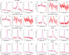 |
Fig. A.1 Spectra of Brγ, Pfγ, and Brα (red line) for the Class II sources observed with SpeX. The fitted continuum is shown as a blue solid line. When the line is considered a detection, the Gaussian fit used to estimate the flux is shown as a dashed line. |
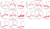 |
Fig. A.3 Continued. |
Appendix B Lacc-L(Brγ) correlation in Class II
As discussed in Sect. 3.2, several literature studies have reported correlations between the accretion rate luminosity, Lαcc, and the intrinsic, extinction corrected Brγ line luminosity, L(Brγ). The most complete and widely used studies are the one by Alcalá et al. (2017) for stars below about one solar mass, and the one by Fairlamb et al. (2017) for intermediate mass stars. None of these two studies covers the full range of LBrγ measured in our sample of Class II, and since the two correlations presented in the literature show small, but significant differences we decided to recompute a correlation optimized for our range of measured line luminosities.
In Figure B.1 we show the samples of Lacc and L(Brγ) measurements from Alcalá et al. (2017) and Fairlamb et al. (2017), the literature fits to the two separate samples, and our combined fit in the line luminosity range −5.5 ≤L(Brγ)/L⊙ ≤ 0.5. In deriving the fit, we only considered the good measurements reported in the literature, excluding upper limits in any of the two quantities. To perform the fit, we used the methodology described in Kelly (2007), using the Python implementation available at https://github.com/jmeyers314/linmix.git. The correlation, and its uncertainties, that we derived for use in this paper is
 (B.1)
(B.1)
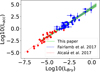 |
Fig. B.1 Correlation of Lacc-LBrγ for Class II objects in the literature. In red we show measurements for stars below about one solar mass (from Alcalá et al. 2017), in blue for intermediate mass stars (from Fairlamb et al. 2017). The red dotted line and blue dashed lines show the literature correlations, derived for each sample separately. The light green line shows the correlation we derive for the range −5.5 ≤ (LBrγ/L⊙) ≤ 0.5. The dark green band shows the uncertainty in the fit. |
All Tables
Properties of the newly observed Class I/F and those from Beck (2007) (below the horizontal line).
All Figures
|
Fig. 1 Top panel: ratio of the de-reddened Brα and Brγ fluxes of Class II sources shown as a function of L★ (left), Lacc, computed from the Brγ luminosity (center; see Sect. 3.3), and the extinction in the K band (right). Bottom panel: same but for the ratio of Pfγ to Brγ fluxes. The values of the ratios are shown by filled dots; the 3σ upper limits are indicated by arrows. When not visible, the errors are smaller than the dots. In both sets of panels, the mean values of the ratios and their uncertainties are shown in orange. |
| In the text | |
|
Fig. 2 Accretion luminosity, Lacc, derived from the Brγ luminosity (Eq. (1)) plotted as a function of the line luminosity for Brα (left panel) and Pfγ (right panel), respectively. The orange line and shadowed area show the best-fitting correlation and their uncertainty (see Eqs. (2) and (3)). |
| In the text | |
|
Fig. 3 Top panel: values of the accretion luminosity, Lacc, derived from L(Brα) as a function of Lacc derived from L(Brγ). Bottom panel: same but for Lacc derived from L(Pfγ). The line of equal values is shown in orange in each panel. |
| In the text | |
|
Fig. 4 Accretion luminosity computed from Pfγ shown as a function of the accretion luminosity computed from Brα for Class I objects. In the first case, the extinction is derived from the ratio Pfγ/Brγ, and in the second it is from Brα/Brγ (see Sect. 4.1). Dark blue dots are objects in Ophiuchus; light blue dots are objects in Taurus. Light blue squares are Taurus objects from Beck (2007). The green dashed line shows the locus of equal values. |
| In the text | |
|
Fig. 5 Extinction in the K band computed from the ratio Pfγ/Brγ is shown versus the value derived from the Brα/Brγ ratio (see Sect. 4.1). Symbols are as in Fig. 4. The green dashed line shows the locus of equal values. |
| In the text | |
|
Fig. 6 Bolometric temperature plotted against the computed foreground extinction (AK,fg). Symbols are as in Fig. 4. |
| In the text | |
|
Fig. 7 Accretion luminosity (top) and fraction of accretion luminosity over bolometric luminosity (bottom) as a function of Lbol. Symbols are as in Fig. 4. The green dotted lines show the locus of Lacc/Lbol=l, 0.1, and 0.01, as marked. |
| In the text | |
|
Fig. 8 Ratio of the accretion luminosity to the bolometric luminosity as a function of Tbol. Symbols are as in Fig. 4. The dotted green lines show the Tbol=700 K and the Lacc=Lbol locus. |
| In the text | |
|
Fig. 9 Top panel: ratio of Lacc/Lbol versus the local extinction in the K band AK,local. Bottom panel: Tbol versus AK,local. Symbols are as in Fig. 4. |
| In the text | |
|
Fig. 10 Ratio of Lacc/Ltot versus age (top) and Ltot (bottom) from the simulations of Lebreuilly et al. (2024). |
| In the text | |
|
Fig. A.1 Spectra of Brγ, Pfγ, and Brα (red line) for the Class II sources observed with SpeX. The fitted continuum is shown as a blue solid line. When the line is considered a detection, the Gaussian fit used to estimate the flux is shown as a dashed line. |
| In the text | |
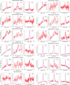 |
Fig. A.2 Same as Fig. A.1 but for Class I sources observed with SpeX. |
| In the text | |
|
Fig. A.3 Continued. |
| In the text | |
|
Fig. B.1 Correlation of Lacc-LBrγ for Class II objects in the literature. In red we show measurements for stars below about one solar mass (from Alcalá et al. 2017), in blue for intermediate mass stars (from Fairlamb et al. 2017). The red dotted line and blue dashed lines show the literature correlations, derived for each sample separately. The light green line shows the correlation we derive for the range −5.5 ≤ (LBrγ/L⊙) ≤ 0.5. The dark green band shows the uncertainty in the fit. |
| In the text | |
Current usage metrics show cumulative count of Article Views (full-text article views including HTML views, PDF and ePub downloads, according to the available data) and Abstracts Views on Vision4Press platform.
Data correspond to usage on the plateform after 2015. The current usage metrics is available 48-96 hours after online publication and is updated daily on week days.
Initial download of the metrics may take a while.