| Issue |
A&A
Volume 703, November 2025
|
|
|---|---|---|
| Article Number | A258 | |
| Number of page(s) | 16 | |
| Section | Planets, planetary systems, and small bodies | |
| DOI | https://doi.org/10.1051/0004-6361/202555168 | |
| Published online | 24 November 2025 | |
Detection and characterisation of a 106-day transiting Jupiter: TOI-2449 b/NGTS-36 b★
1
Leiden Observatory, Leiden University,
PO.Box 9513,
2300 RA
Leiden,
The Netherlands
2
Observatoire Astronomique de l’Université de Genève,
Chemin Pegasi 51b,
1290
Versoix,
Switzerland
3
Space Research and Planetary Sciences, Physics Institute, University of Bern,
Gesellschaftsstrasse 6,
3012
Bern,
Switzerland
4
Department of Physics, University of Warwick,
Gibbet Hill Road,
Coventry
CV4 7AL,
UK
5
Centre for Exoplanets and Habitability, University of Warwick,
Gibbet Hill Road,
Coventry
CV4 7AL,
UK
6
Millennium Institute for Astrophysics,
Santiago,
Chile
7
Facultad de Ingeniería y Ciencias, Universidad Adolfo Ibáñez,
Av. Diagonal las Torres 2640,
Peñalolén, Santiago,
Chile
8
Data Observatory Foundation,
Santiago,
Chile
9
Instituto de Astrofísica e Ciências do Espaço, Universidade do Porto,
CAUP, Rua das Estrelas,
4150-762
Porto,
Portugal
10
Instituto de Astronomía, Universidad Católica del Norte,
Angamos 0610,
1270709,
Antofagasta,
Chile
11
Astronomy Unit, Queen Mary University of London,
G.O. Jones Building, Bethnal Green,
London
E1 4NS,
UK
12
Space Research Institute, Austrian Academy of Sciences,
Schmiedl-strasse 6,
8042
Graz,
Austria
13
Cerro Tololo Inter-American Observatory,
Casilla 603,
La Serena,
Chile
14
Mullard Space Science Laboratory, University College London,
Holmbury St Mary, Dorking,
Surrey
RH5 6NT,
UK
15
School of Physics and Astronomy, University of Leicester,
Leicester
LE1 7RH,
UK
16
Center for Astrophysics || Harvard & Smithsonian,
60 Garden Street,
Cambridge,
MA
02138,
USA
17
Max-Planck-Institut für Astronomie,
Königstuhl 17,
69117
Heidelberg,
Germany
18
Space Telescope Science Institute,
3700 San Martin Drive,
Baltimore,
MD
21218,
USA
19
Department of Space, Earth and Environment, Chalmers University of Technology, Onsala Space Observatory,
439 92
Onsala,
Sweden
20
NASA Exoplanet Science Institute, Caltech/IPAC,
Mail Code 100-22, 1200 E. California Blvd.,
Pasadena,
CA
91125,
USA
21
Department of Physics and Kavli Institute for Astrophysics and Space Research, Massachusetts Institute of Technology,
Cambridge,
MA
02139,
USA
22
University of Zurich, Department of Astrophysics,
Winterthurerstr. 190,
8057
Zurich,
Switzerland
23
NASA Ames Research Center,
Moffett Field,
CA
94035,
USA
24
SETI Institute,
Mountain View,
CA
94043,
USA
25
Instituto de Estudios Astrofísicos, Facultad de Ingeniería y Ciencias, Universidad Diego Portales,
Av. Ejército 441,
Santiago,
Chile
26
Centro de Astrofísica y Tecnologías Afines (CATA),
Casilla 36-D,
Santiago,
Chile
27
ESO – European Southern Observatory,
Av. Alonso de Cordova 3107,
Vitacura, Santiago,
Chile
28
Department of Physics and Astronomy, The University of North Carolina at Chapel Hill,
Chapel Hill,
NC 27599-3255,
USA
29
Bay Area Environmental Research Institute,
Moffett Field,
CA
94035,
USA
30
Center for Space and Habitability, University of Bern,
Gesellschaftsstrasse 6,
3012
Bern,
Switzerland
31
STAR Institute, Université de Liège,
Liège,
Belgium
32
Institute of Space Sciences (ICE, CSIC),
Carrer de Can Magrans S/N, Campus UAB,
Cerdanyola del Valles,
08193
Spain
33
Institut d’Estudis Espacials de Catalunya (IEEC),
08860
Castellde-fels (Barcelona),
Spain
34
Astrophysics Research Centre, School of Mathematics and Physics, Queen’s University Belfast,
Belfast
BT7 1NN,
UK
35
Center for Data Intensive and Time Domain Astronomy, Department of Physics and Astronomy, Michigan State University,
East Lansing,
MI
48824,
USA
36
Instituto de Astrofísica, Facultad de Física, Pontificia Universidad Católica de Chile,
Av. Vicuña Mackenna
4860,
Santiago,
Chile
37
Department of Astronomy/Steward Observatory, The University of Arizona,
933 North Cherry Avenue,
Tucson,
AZ
85721,
USA
38
Department of Earth, Atmospheric and Planetary Sciences, Massachusetts Institute of Technology,
Cambridge,
MA
02139,
USA
39
Department of Aeronautics and Astronautics, MIT,
77 Massachusetts Avenue,
Cambridge,
MA
02139,
USA
40
Departamento de Física e Astronomia, Faculdade de Ciências, Universidade do Porto,
Rua do Campo Alegre,
4169-007
Porto,
Portugal
41
Department of Astronomy, The Ohio State University,
140 W. 18th Ave.,
Columbus,
OH
43210,
USA
42
Landessternwarte, Zentrum für Astronomie der Universtät Heidelberg,
Königstuhl 12,
69117
Heidelberg,
Germany
43
Department of Astronomy, Sofia University St Kliment Ohridski,
5 James Bourchier Blvd,
1164
Sofia,
Bulgaria
44
Institute of Physics, École Polytechnique Fédérale de Lausanne (EPFL),
Observatoire de Sauverny, Chemin Pegasi 51b,
1290
Versoix,
Switzerland
45
Department of Astrophysical Sciences, Princeton University,
Princeton,
NJ
08544,
USA
46
University of Southern Queensland, Centre for Astrophysics,
West Street,
Toowoomba,
QLD 4350,
Australia
47
Department of Physics, Engineering and Astronomy, Stephen F. Austin State University,
1936 North St,
Nacogdoches,
TX
75962,
USA
★★ Corresponding author: This email address is being protected from spambots. You need JavaScript enabled to view it.
Received:
15
April
2025
Accepted:
18
September
2025
Abstract
Context. Only a handful of transiting giant exoplanets with orbital periods longer than 100 days are known. These warm exoplanets are valuable objects, as their radius and mass can be measured and lead to an in-depth characterisation of the planet’s properties. Thanks to low levels of stellar irradiation and large orbital distances, the atmospheric properties and orbital parameters of warm exoplanets remain relatively unaltered by their host star, giving new insights into planetary formation and evolution.
Aims. Our aim is to increase the sample of warm giant exoplanets with precise radii and masses. Our goal is to identify suitable candidates in the Transiting Exoplanet Survey Satellite data and perform follow-up observations with ground-based instruments.
Methods. We used the Next Generation Transit Survey (NGTS) to detect additional transits of planetary candidates in order to pinpoint their orbital period. We also monitored the target with several high-resolution spectrographs to measure the planetary mass and eccentricity. We studied the planet’s interior composition with a planetary evolution code to determine the planet’s metallicity.
Results. We report the discovery of a 106-day period Jupiter-sized planet around the G-type star TOI-2449/NGTS-36. We jointly modelled the photometric and radial velocity data and find that the planet has a mass of 0.70−0.04+0.05 MJ and a radius of 1.001 ± 0.009 RJ. The planetary orbit has a semi-major axis of 0.449 au and is slightly eccentric (e = 0.0098−0.030+0.028). We detected an additional 3-year signal in the radial velocity data that is likely due to the stellar magnetic cycle. Based on the planetary evolution models considered here, we find that TOI-2449 b/NGTS-36 b contains 11−5+6 M⊕ of heavy elements and has a marginal planet-to-star metal enrichment of 3.3−1.8+2.5. Assuming a Jupiter-like bond albedo, TOI-2449 b/NGTS-36 b has an equilibrium temperature of 400 K and is a good target for understanding nitrogen chemistry in cooler atmospheres.
Key words: methods: data analysis / planets and satellites: detection / planets and satellites: gaseous planets / planets and satellites: individual: TOI-2449b
Based on observations collected at the European Southern Observatory under ESO programmes: 105.20GX.001, 106.21ER.001, 108.22A8.001, 108.22L8.001, 109.239V.001, 110.23YQ.001.
Oort Postdoctoral Fellow.
SNSF Postdoctoral Fellow.
© The Authors 2025
 Open Access article, published by EDP Sciences, under the terms of the Creative Commons Attribution License (https://creativecommons.org/licenses/by/4.0), which permits unrestricted use, distribution, and reproduction in any medium, provided the original work is properly cited.
This article is published in open access under the Subscribe to Open model. This email address is being protected from spambots. You need JavaScript enabled to view it. to support open access publication.
1 Introduction
Gas giant exoplanets play a crucial role in the formation and evolution of planetary systems. They form within the first 10 Myr, before the gas disc dissipates (e.g. Mordasini & Burn 2024), and contain the majority of the mass of a planetary system. Gas giants are known to shape the architecture of planetary systems (e.g. Levison & Agnor 2003; Kong et al. 2024), but the exact role of giant planets and the mechanisms driving their formation and migration remain to be understood.
The discovery of close-in giant exoplanets with orbital periods of a few days (e.g. Mayor & Queloz 1995) brought more questions with regard to their formation and migration pathways. Two types of models are usually considered: in situ formation (e.g. Bodenheimer et al. 2000) and ex situ formation, in which the gas giants must have formed at large distances from the host stars and migrated inward in order to arrive at their current locations (e.g. Lin et al. 1996). Several migration scenarios are needed to explain the range of orbital periods and eccentricities at which these giant planets are found. Generally, the two main channels envisioned are high-eccentricity migration (e.g. Rasio & Ford 1996) and disc migration (e.g. Goldreich & Tremaine 1980; Baruteau et al. 2014 for a review).
Studying the orbital architecture and stellar obliquities (spinorbit angles) of close-in giant planets in particular are key to understanding which migration scenarios are needed to reproduce the observed population. Transiting exoplanets are excellent probes to determine projected spin-orbit angles, which are often measured with observations of the Rossiter-McLaughlin effect.
Unfortunately, the orbital and physical parameters of hot Jupiters, planets with orbital period shorter than 10 days, are largely influenced by the interactions with their host star, which can change their original properties. Hot Jupiters are subject to strong tidal interactions with their host star, which dampens their orbital eccentricity and could dampen stellar obliquities (e.g. Albrecht et al. 2012, 2022). Hot Jupiters also have larger radii than expected, as seen in interior structure modelling, due to their proximity to the host star and the intense stellar irradiation they receive. Dawson & Johnson (2018) review the mechanisms leading to the inflation of hot Jupiter radii.
In contrast to hot Jupiters, warm Jupiters, usually defined as planets with orbital periods between 10 and 200 days (e.g. Dawson & Johnson 2018; Wang et al. 2024), are less susceptible to stellar interactions and likely retain their post formation and migration characteristics. The sample of well characterised warm Jupiters is still relatively small: 90 warm giant planets have precise masses and radii (uncertainty less than 25% and 8%, respectively)1. Since its launch in December 2018, the Transiting Exoplanet Survey Satellite (TESS) satellite (Ricker et al. 2015) has been conducting a near all sky survey with 27-day long pointings. Towards the poles, the pointings overlap to provide an uninterrupted observation of up to one year. Most transiting warm Jupiters appear as a single transit event in a given pointing. Villanueva et al. (2019) and Cooke et al. (2019) have pointed out the need to identify single or duo transit events in order to discover long-period planets and published predicted yields. From simulations including TESS Year 1 and 3 light curves, Rodel et al. (2024) find that about 110 planets with orbital periods larger than 100 days should be detected and that 75% of those will be monotransits.
Long-term radial velocity campaigns have enabled mass and eccentricity measurements for these transiting planets and have led to well-characterised systems (e.g. Schlecker et al. 2020; Hobson et al. 2021; Eberhardt et al. 2023; Ulmer-Moll et al. 2023; Brahm et al. 2023). Photometric follow-up campaigns are also required to recover the orbital period of warm transiting planets. Citizen scientists are involved in this effort, both in the identification of single transit events (e.g. TOI-2180 b, a 260-day planet; Dalba et al. 2022) and the photometric observations of candidates (e.g. Sgro et al. 2024). The Next Generation Transit Survey (NGTS; Wheatley et al. 2018) has a multi-year monitoring program of single and duo transit candidates that has led to the discovery of several transiting warm Jupiters with orbital periods ranging from just above 20 days to up to 100 days (e.g. Gill et al. 2020; Ulmer-Moll et al. 2022; Battley et al. 2024).
In this context, we report the discovery of a transiting warm Jupiter orbiting TOI-2449 characterised with TESS and NGTS data and radial velocity data. In Sect. 2 we present the photometric data, radial velocities, and high-resolution imaging data. The methods for the determination of the stellar and planetary parameters are detailed in Sect. 3. In Sect. 4 we present the results of the joint photometric and radial velocity fit, and we determine the heavy element mass of TOI-2449 b. Finally, we discuss and summarise our work in Sects. 5 and 6.
2 Observations
TOI-2449 was observed by TESS (Sect. 2.1) and follow-up photometric observations were obtained with NGTS (Sect. 2.2). Ground-based spectroscopic observations were carried out with the high-resolution spectrographs CHIRON, CORALIE, FEROS, and HARPS, which are presented in Sects. 2.4, 2.3, 2.5, and 2.6, respectively. High-resolution imaging data and results are detailed in Sects. 2.7 and 2.8.
2.1 TESS photometry
The Transiting Exoplanet Survey Satellite (Ricker et al. 2015) is a photometric survey mission that scans almost the entire sky. TOI-2449 was observed by TESS in sectors 4 and 5 (from October 19 to December 11, 2018) at a two-minute cadence and in sectors 31 and 32 (from October 22 to December 16, 2020) at a cadence of 10 minutes.
TOI-2449 b was first announced as a TESS object of interest (TOI) on January 6, 2021, with a single transit event detected in sector 31 by the Quick Look Pipeline (QLP) at MIT (Huang et al. 2020a,b). We obtained the light curves from the four TESS sectors through the Mikulski Archive for Space Telescopes (MAST) archive2. We downloaded the outputs of the Science Processing Operation Center (SPOC; Jenkins et al. 2016) pipeline, and we used the pre-search data conditioning simple aperture photometry (PDCSAP; Stumpe et al. 2012; Smith et al. 2012; Stumpe et al. 2014) in our analysis. The image data were reduced and analysed by SPOC at the NASA Ames Research Center. The PDCSAP light curves were corrected for dilution and for systematic trends shared by other stars on the detector.
We checked for contaminant sources in the aperture with the tpfplotter software package (Aller et al. 2020). No neighbouring sources were found down to a G magnitude difference of eight for the four TESS sectors. The two nearest neighboring stars have flux ratios of 0.0032 and 0.0009 in the G band. We include the figure of the TESS target pixel file for sector 31 in Appendix A.
2.2 NGTS photometry
The Next Generation Transit Survey operates a set of twelve robotic telescopes located at Cerro Paranal, Chile. Each unit is a 20 cm telescope fitted with back-illuminated deep-depletion CCD cameras (Wheatley et al. 2018). NGTS uses a custom filter ranging from 520 to 890 nm. For TOI-2449, with a T-band magnitude of 9.9, the expected photometric precision for a single NGTS telescope is 400 ppm per 30 mins. At a T-band magnitude brighter than 9.5, the 12 NGTS telescopes reach a photometric precision of 100 ppm per 30 mins (e.g. Bryant et al. 2020; O’Brien et al. 2021).
After the release of the new transiting candidate around TOI-2449, the target was included in the on-going NGTS program aimed at the discovery of warm and temperate exoplanets. TOI-2449 was monitored for a first campaign that resulted in 80 nights of observations with one NGTS camera from January 15 to April 23, 2021. No transit event was detected in this first NGTS campaign. The second campaign consisted of 94 nights of observations with one NGTS camera from July 5 to December 3, 2021. One partial transit matching the transit depth of the transiting event in TESS was identified on September 14, 2021. After this detection, the maximum possible period was 318.4 days, and five period aliases (all above 50 days) were still compatible with the TESS and NGTS data. A second partial transit was observed on November 13, 2022, with six cameras based on the radial velocity solution. This third transit reduced the set of possible orbital periods to only two period aliases: 53.07 and 106.14 days. During the first transit observation, the photometric precision was 380 ppm per 30 mins. During the second transit observations, the 30-minute photometric precision was between 530 and 680 ppm per camera. The seeing and wind speed were higher during this second observation and probably impacted the photometric precision. The NGTS data shows a long-term decreasing trend that cannot be attributed to instrumental effects and is likely due to long-term stellar activity. The nightly binned NGTS data are presented in Fig. B.1 along with three selected nights showing light curves with and without a transit detection.
2.3 CORALIE spectroscopy
We used the CORALIE spectrograph (Baranne et al. 1996; Queloz et al. 2001b; Ségransan et al. 2010) to first confirm the planetary nature of TOI-2449 b and then monitor the radial velocity of the target for two years. CORALIE is a highresolution fibre-fed spectrograph installed at the Swiss Euler 1.2m telescope3 located in La Silla, Chile. CORALIE has a spectral resolution of 60 000 with a sampling per resolution element equal to three pixels. CORALIE is fed by two fibres. The first fibre is used for science observation, and the second fibre is used either to observe a Fabry–Pérot étalon for drift calibration purposes or to observe the sky for background subtraction. We observed TOI-2449 together with the simultaneous Fabry-Pérot étalon.
We obtained 32 CORALIE spectra of TOI-2449 from January 17, 2021, to March 11, 2023, with exposure times varying between 900 and 1800 seconds. The objectives of the radial velocity observations are to rule out spectroscopic binaries with the first two CORALIE measurements and then to detect the reflex motion induced by the transiting candidate with a monitoring over several months with a radial velocity precision of about 10 m s−1. The spectra were reduced with the standard data reduction pipeline and cross-correlated with a G2-type stellar mask to obtain the radial velocity measurements and associated errors (e.g. Pepe et al. 2002). The radial velocities are presented in Table 1. Along with the radial velocities, the pipeline provides useful parameters that can be used as stellar activity indicators: the full width half maximum (FWHM), contrast, and bisector inverse slope (BIS; Queloz et al. 2001a) of the cross-correlation function (CCF).
2.4 CHIRON spectroscopy
CHIRON is a fibre-fed high-resolution spectrograph installed at the 1.5m telescope located in Cerro Tololo INter-american Observatory, Chile (Tokovinin et al. 2013). CHIRON monitored TOI-2449 for one year, from January 8, 2021, to January 29, 2022, collecting 72 observations with an exposure time varying between 900 and 1200 seconds, leading to a signal-to-noise ratio per extracted pixel between 17 and 40, depending on the atmospheric conditions and air mass. Spectral extraction and calibration was performed via the standard CHIRON pipeline (Paredes et al. 2021). Line profiles and radial velocities were determined from each spectrum via a least-squares deconvolution between the observed spectrum and a synthetic non-rotating template, generated from ATLAS9 model atmospheres (Castelli & Kurucz 2003). Radial and line broadening velocities are determined by modelling the line profiles with an analytic broadening kernel that encompasses the effects of rotational, macroturbulence, and instrumental broadening, as per Gray (2005). The radial velocity measurements are reported in Table 1.
Radial velocities of TOI-2449 (extract).
2.5 FEROS spectroscopy
TOI-2449 was also monitored by the Fiber-fed Extended Range Optical Spectrograph (FEROS), located at the 2.2 m telescope in La Silla, Chile. FEROS has a resolution of 48 000 and covers the optical range from 360 to 920 nm (Kaufer et al. 1999). TOI-2449 was observed over two years, comprising 17 observations under the programs 0106.A-9014, 0107.A-9003, 0108.A-9003, and 0109.A-9003. The observations were done using the simultaneous wavelength calibration mode with an average exposure time of 300 seconds, leading to spectra with a typical signal-to-noise ratio per resolution element between 60 and 90. The data were reduced with the CERES pipeline (Brahm et al. 2017), which provides the radial velocity measurement and associated error as well as the FWHM and BIS of the CCF. The radial velocity measurements are listed in Table 1.
2.6 HARPS spectroscopy
HARPS is a high-resolution fibre-fed spectrograph installed at the European Southern Observatory (ESO) 3.6 m telescope at La Silla, Chile (Mayor et al. 2003). Given that CORALIE, CHIRON, and FEROS observations hinted at the detection of a planet around TOI-2449, additional observations were acquired with HARPS in order to refine the orbital solution and planetary parameters with a radial velocity precision at the meter per second level. During two years, we used the HARPS spectrograph to monitor TOI-2449 with the high-accuracy mode and exposure times varying between 900 and 1200 seconds, depending on the weather conditions. TOI-2449 was observed for a total of 55 observations under several programs aiming to confirm transiting warm Jupiters: 105.20GX.001, 106.21ER.001, 108.22L8.001, 108.22A8.001, 109.239V.001, and 110.23YQ.001. The HARPS data were reduced with the standard data reduction pipeline, and the radial velocities were obtained with the cross-correlation technique using a G2 mask. The radial velocity measurements are reported in Table 1. The HARPS spectra were co-added and then used to perform the stellar analysis in Sect. 3.1.
2.7 Zorro imaging
High-resolution imaging is one of the critical assets required as part of the validation and confirmation process for a transiting exoplanet observation. The presence of a close companion star, whether truly bound or along the line of sight, causes additional light contamination of the observed transit, leading to derived properties for the exoplanet and host star that are incorrect (Ciardi et al. 2015; Furlan & Howell 2017, 2020). Given that nearly one-half of FGK stars are in binary or multiple star systems (Matson et al. 2018), high-resolution imaging yields crucial information towards our understanding of each discovered exoplanet as well as more global information on exoplanetary formation, dynamics, and evolution (Howell et al. 2021).
TOI-2449 was observed on September 22, 2021, using the Zorro speckle instrument on Gemini South (Scott et al. 2021). Zorro provides simultaneous speckle imaging in two bands (562 nm and 832 nm), and its output data products include a reconstructed image and robust contrast limits on companion detections (Howell et al. 2011). Seven sets of 1000 × 0.06 sec exposures were collected and subjected to Fourier analysis using the Zorro standard data reduction pipeline. Figure C.1 shows the resulting 5 σ contrast curves and the 832 nm reconstructed speckle image. We find that TOI-2449 is a single star with no close companion brighter than five to seven magnitudes from the diffraction limit ( 20 mas) out to 1.2J. At the distance of TOI-2449, these angular limits correspond to spatial limits of 3–188 au.
2.8 SOAR imaging
We also searched for stellar companions of TOI-2449 with speckle imaging on the 4.1-m Southern Astrophysical Research (SOAR) telescope (Tokovinin 2018) on February 27, 2021, observing in the Cousins I-band, an overlapping visible bandpass similar to TESS. This observation was sensitive to a 5.8-magnitude fainter star at an angular distance of 1 arcsec from the target. More details of the observation are available in Ziegler et al. (2020). The 5 σ detection sensitivity and speckle auto-correlation functions from the observations are shown in Fig. C.2. No nearby stars were detected within 3″ of TOI-2449 in the SOAR observations.
3 Methods
3.1 Stellar parameter determination
We used the ARES+MOOG method described by Sousa et al. 2021; Sousa 2014; Santos et al. 2013 to obtain the stellar spectroscopic parameters (Teff, log 𝑔, microturbulence, [Fe/H]). The equivalent widths were measured using the ARES code4 (Sousa et al. 2007, 2015). For this spectral analysis, we used a combined HARPS spectrum of TOI-2449 (S/N = 250) to measure the equivalent widths for the list of lines presented in Sousa et al. (2008). The best set of spectroscopic parameters for each spectrum was found by using a minimisation process to find the ionisation and excitation equilibrium. This process makes use of a grid of Kurucz model atmospheres (Kurucz 1993) and the latest version of the radiative transfer code MOOG (Sneden 1973). We also derived a more accurate trigonometric surface gravity (adopted value) using recent Gaia data. We matched the star with the Gaia ID in DR3 using their coordinates and the VizieR catalogues (I/355/gaiadr3, Gaia Collaboration 2023). We followed the same procedure as described in Sousa et al. (2021), which provided a consistent value when compared with the spectroscopic surface gravity.
To determine the stellar radius of TOI-2449, we utilised a Markov chain Monte Carlo modified infrared flux method (IRFM – Blackwell & Shallis 1977; Schanche et al. 2020). Within this approach we computed synthetic photometry from constructed spectral energy distributions built from two atmospheric model catalogues (Kurucz 1993; Castelli & Kurucz 2003) that were constrained using our stellar spectral results. These synthetic fluxes were compared to broadband observations in the passbands Gaia G, GBP, and GRP; 2MASS J, H, and K; and WISE W1 and W2 (Skrutskie et al. 2006; Wright et al. 2010; Gaia Collaboration 2023) to derive the stellar bolometric flux. From this we obtained the stellar effective temperature and angular diameter that was converted into the stellar radius using the offset-corrected Gaia parallax (Lindegren et al. 2021). We conducted a Bayesian model averaging of the radius posterior distribution from the individual atmospheric catalogues to account for model uncertainties.
The stellar effective temperature, metallicity, and radius constitute the basic input set we used to derive the stellar mass, M★, and age, t★, with two different stellar evolutionary codes. We first used the isochrone placement algorithm (Bonfanti et al. 2015, 2016) and its capability of interpolating the input parameters within pre-computed grids of PARSEC5 v1.2S (Marigo et al. 2017) isochrone and tracks. As detailed in Bonfanti et al. (2016), to enhance convergence we further input υ sin i★ as a proxy for the stellar rotation period and benefited from the synergy between the isochrone fitting and the gyrochronological relation from Barnes (2010) to get an initial pair of mass and age estimates. A second pair of estimates were derived by the CLES (Code Liègeois d’Évolution Stellaire; Scuflaire et al. 2008) code, which generates the best-fit stellar evolutionary track following a Levenberg–Marquadt minimisation scheme constrained by the basic set of input parameters (see Salmon et al. 2021). The two stellar evolutionary codes led to stellar masses of M★ = 1.065 ± 0.049 M⊙ with PARSEC and M★ = 1.091 ± 0.041 M⊙ with CLES, and stellar ages of t★ = 2.8 ± 1.3 Gyr with PAR-SEC and t★ = 2.1 ± 1.5 Gyr with CLES. After checking the mutual consistency of the two respective pairs of outcomes with the χ2 -based criterion outlined in Bonfanti et al. (2021), we combined the two mass and age distributions, and we obtained  and
and  Gyr (see Bonfanti et al. 2021, for further details). The results are presented in Table 2.
3.2 Radial velocity analysis
3.2.1 Search for periodic signals
As described in Sect. 2, following the announcement of transiting candidate TOI-2449 b, the host star was observed by four high-resolution spectrographs covering a time span of 1136 days. The radial velocity data were first analysed to search for the signal of the transiting planet and potential additional planets. The full dataset of radial velocities and the generalised Lomb–Scargle periodogram are presented in Fig. 1. This first periodogram shows a clear detection of a periodic signal with a wide peak around 106 days. This periodicity is in line with the period alias at 106.14 days of the transiting candidate found in the TESS and NGTS data. There is no significant periodic signal around the other period alias at 53 days, so we assigned the photometric detection and this radial velocity signal to the same object: a transiting planet at 106 days. To search for additional signals, we subtracted the best-fit sinusoid with the period corresponding to the highest power (106 days) from the radial velocity data. We then re-computed the periodogram and selected the next-highest peak that exceeds the 1% false alarm probability. We repeated this procedure until no peak was detected above the 1% false alarm probability. We found a second significant signal at around 1100 days, which is similar to the time span of the data, and a third significant signal at 34 days. Figure 2 displays the periodogram in period space of the whole radial velocity dataset, the activity indicators and the periods mentioned previously are highlighted. The activity indicators were computed from the CORALIE, FEROS, and HARPS spectra only. We note that the signal-to-noise of some spectra are too low to compute reliable values.
We ran a radial velocity only analysis to determine if a model with three planetary signals would be the preferred model. We used kima (Faria et al. 2018), a software package that allows one to fit for the number of planets as a free parameter, along with all the parameters describing the Keplerian orbits and instrument offsets and jitters. We used a uniform prior on the number of planets from zero to three planets. The priors for the other parameters are detailed in Table D.1, and in particular we note that we set a LogUniform prior for the orbital period ranging from 1 to 3000 days (slightly more than 2.5 times the span of the radial velocity data). After running our model with kima, we obtained an effective sample size (ESS) of 22 790, with no samples for the no-planet nor the one-planet model.
We found that a two-planet model is largely favoured over all the other models by comparing the probabilities. The Bayes factor of the two-planet versus the one-planet model is larger than the ESS of 22 790, which is largely above the usual threshold of 150 cited for a decisive detection (e.g. Feroz et al. 2011). The Bayes factor of the three-planet model versus the two-planet model is only of 0.14, demonstrating that there is not enough evidence to claim the detection of a third signal.
Only two signals were confidently detected when modelled as Keplerian functions with kima. The posterior distribution of the orbital periods is shown in Fig. 3, displaying two peaks close to 106 and 1140 days. In the periodogram search, the 34-day signal has a relatively high probability (about 1%) of being a false alarm when compared to the first two signals detected: The false alarm probabilities are 10−52 and 10−16 for the 106 and 1100-day signals, respectively. Hence the 34-day signal is less significant and could be due to the sensitivity of the periodogram to the choice of noise model (e.g. Delisle et al. 2020). It is also worth mentioning that in the kima analysis, the orbital period priors are wide (see Table D.1), which may result in conservative Bayes factor values when comparing the two- and three-planet models.
We note that the 34-day signal originally found in the periodogram search could be explained as an alias of the stellar rotation period. Using the log R′HK, we estimated the stellar rotation to be 16 ± 3 days (Eqs. (3) and (4) from Noyes et al. 1984). We computed the periodogram of the NGTS data, and we found hints of a 16-day periodic signal in the second season of the data but not in the first one. For the first signal, we retrieved an orbital period of  days, which is in agreement with one period alias of the transiting object (106.143 days) within 1σ. We independently detected the reflex motion of the transiting candidate, thus confirming the detection of a 106-day planet around TOI-2449. For the second signal, the posterior distribution of the orbital period is less constrained and results in an orbital period of
  days. While the origin of the first signal is clear and in line with the transiting candidate detected in the photometric data, the origin of the second signal with a period of about 3 years remains to be determined.
Stellar properties and stellar parameters.
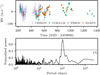 |
Fig. 1 Radial velocities of TOI-2449. Top: radial velocity data spanning 1136 days (CHIRON, blue; CORALIE, green; FEROS, grey; HARPS, orange). Bottom: generalised Lomb-Scargle periodogram of the radial velocities. The black line marks the 1% false alarm probability. |
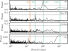 |
Fig. 2 Generalised Lomb–Scargle periodogram of the radial velocities, the radial velocity residuals after joint modelling (see Sect. 3.3), FWHM of the CCF, and Hα indicator. Vertical lines highlight the relevant periods (red: stellar rotation; green: significant signals). The grey line marks the 1 % false alarm probability. |
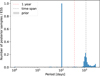 |
Fig. 3 Posterior distribution of the orbital period for a model with up to three planets (blue histogram). The prior on the orbital period is identical for the three planets and shown in grey. The ESS is equal to 22 790 samples. |
3.2.2 Possible origin of the 3-year signal
We investigated if the signal at  days could be associated with the stellar magnetic cycle. Suárez Mascareño et al. (2016) report in their combined study of 150 stars the statistics on the length of known magnetic cycles. Based on 55 G-type stars, the authors find that the distribution of cycle length peaks between 2 and 4 years and then slowly decrease until 12 years. They also report that the median length of a cycle is 6 ± 3.6 years. Regarding the stellar rotation period, the G stars in their sample have a median rotation period of 18.4 ± 11.1 days. These values are well in agreement with what we measured for TOI-2449: a G0/G1-type star with a stellar rotation period of 16 ± 3 days and a potential magnetic cycle of
  years.
Isaacson et al. (2024) report on the search for activity cycles in 285 stars from the California Legacy Survey. The authors detected activity cycles for 138 stars in their sample. For the 29 G-stars with detected activity cycles, they find that the periods of the activity cycle range from 3.9 to 23 years, and the stellar rotation periods range from 14 to 34 days. Interestingly, they find tightly constrained cycle periods for stars with log(R′HK) between −4.7 and −4.9. For the more active G-stars, the cycle periods are equal to or less than 5 years, while less active G-stars have cycle periods ranging from 5 to 23 years. With a log(R′HK) of −4.9, an activity cycle of about 3 years for TOI-2449 is coherent with this recent study.
The hypothesis of a 3-year magnetic cycle is supported by the study of the stellar activity indicators derived from the high-resolution spectra of TOI-2449. In Fig. 2, looking first at the FWHM of the CCF, we found no significant periodicity at 106 days, and there is no significant signal close to 1100 days. One indicator has a significant peak close to 1140 days: Hα with a periodicity around 1200 days. Through their work on the Sun as a star, Livingston et al. (2007) reported that CaII K tracks very well the solar magnetic cycle and that other chrosmospheric lines such as Hα trace the same variations as Ca II K. For FGK stars, Ca II and Hα have also been shown to trace long-term activity cycles as well as short-term signals (e.g. Gomes da Silva et al. 2022). Hence, we propose that this 3-year signal is likely emerging from stellar activity and can be attributed to the magnetic cycle of TOI-2449.
3.2.3 Stellar activity modelling
We aimed at choosing the best model for the 3-year signal in the radial velocity data. Using kima, we first modelled our dataset with only the transiting planet TOI-2449 b, setting the prior on the orbital period to a normal distribution around the value obtained from a preliminary fit of the photometric data. Then, we built a second model with the transiting planet and a parametrisation of the 3-year signal as a cubic or a sinusoidal function. We find that a model that accounts for the 3-year signal is largely favoured with a Bayes factor larger than 200. Comparing the cubic versus the sinusoid model, we find that the latter is slightly favoured with a Bayes factor of five.
Finally, we looked at the potential modelling of the activity induced by the stellar rotation period at 16 days, which could produce the third signal at 34 days seen in the periodogram analysis. To do so, we used our previous model containing the transiting planet and a sinusoid function, and we added a Gaussian process (GP) with a quasi-periodic kernel. The maximum likelihood solution is shown in Appendix E.1. We find that this last model leads to a marginal improvement, compared to a model without a GP, with a Bayes factor of only 2.8. We verified that the planetary parameters obtained are consistent with the model without a GP. In particular, the planetary mass is consistent well within 1 σ between the models. Hence, we chose to move forward with a model without a GP, which only accounts for the transiting planet along with the 3-year signal.
3.3 Photometry and radial velocity analysis
We used the software package juliet (Espinoza et al. 2019) to model the photometric and radial velocity data of TOI-2449. Using a Bayesian framework, Juliet allows one to model multi-planet systems with a given number of transiting and non-transiting objects. The planetary transits are modelled with batman (Kreidberg 2015), and the Keplerian signals are modelled with RadVel (Fulton et al. 2018). The stellar activity signals and instrument systematics can be taken into account with parametric functions or Gaussian processes (e.g. Gibson 2014).
We chose to only include TESS sector 31 in our analysis since this sector is the one displaying a transit event. Similarly for the NGTS data, we included in the joint analysis only the nights that display a partial transit event. We specified for the TESS and NGTS photometric filters two sets of quadratic limb-darkening parameters (Kipping 2013). The priors on the limb-darkening parameters were obtained with the LDCU6 code. LDCU is a modified version of the python routine implemented by Espinoza & Jordán (2015) that computes the limb-darkening coefficients and their corresponding uncertainties using a set of stellar intensity profiles accounting for the uncertainties on the stellar parameters. The stellar intensity profiles are generated based on two libraries of synthetic stellar spectra: ATLAS (Kurucz 1979) and PHOENIX (Husser et al. 2013). We used the most conservative estimate from LDCU, which is the merged version of all the results.
We also specified three sets of offset and jitter terms for TESS sector 31 and the two nights of NGTS data because the NGTS data were taken more than one year apart. We did not include a dilution factor for either instrument, as the TESS and NGTS apertures are not contaminated by other sources. To correctly evaluate the baseline of the in-transit data in the TESS photometry, we chose to model the photometric variability with a GP using a Matérn 3/2 kernel. We tested using a SHO kernel with broad log-uniform priors on the scale amplitude, angular frequency, and quality factor. There was no improvement in the fit as measured by the evidence value, and the planetary parameters were all consistent within 1σ.
We modelled the planetary signal with the following parameters: orbital period, planet-to-star radius ratio, mid-transit time, impact parameter, argument of periastron, eccentricity, and radial velocity semi-amplitude. We chose to model the eccentricity and argument of periastron with the  parametrization (Eastman et al. 2013). On top of the reflex motion induced by the transiting planet, the radial velocity data show a long-term signal with a periodicity close to 3 years. This signal is probably induced by the magnetic activity cycle (see Sect. 3.2.2 for more details), and we modelled it with a circular orbit. The data from the four spectrographs CHIRON, CORALIE, FEROS, and HARPS were modelled by specifying an independent set of offset and jitter per instrument. Moreover, we chose to model the stellar density with a normal prior derived from the stellar analysis performed in Sect. 3.1. The priors on all fitted parameters are detailed in Table F.1. We used the nested sampling method dynesty (Speagle 2019) implemented in Juliet with 2000 live points and stopped sampling once the uncertainty on the log-evidence was smaller than 0.1.
4 Results
4.1 Planetary and orbital parameters of TOI-2449 b
We jointly modelled the photometric and radial velocity data of TOI-2449, and we found that this GO-star hosts a transiting planet on a 106-day orbit. The planet TOI-2449 b has the following characteristics: a mass of  MJ and a radius of 1.001 ± 0.009 RJ. The planetary orbit has a semi-major axis of
  au and a small eccentricity of
  . The total transit duration is 8.26 ± 0.06 hours. The full transit of TOI-2449 b observed with TESS at a 10-min cadence and the two partial transits observed with NGTS (one camera in 2021 and six cameras in 2022) binned to a 10-min cadence are presented in Fig. 4. In Fig. G.1, we show the full TESS light curve of sector 31. After subtraction of the median model, the light curves are without structures, and the residuals of the TESS data have a standard deviation of 408 ppm. We verified that the residuals follow a normal distribution by using a Kolmogorov-Smirnov test. We measured the standard deviation of the residuals as a function of the time bins (ranging from 3-hour to 10-minute binning), and we confirmed that the residuals follow the same decreasing trend as samples taken from a normal distribution. The residuals of the first NGTS observation, done with one camera and binned to 10 minutes, has a standard deviation of 460 ppm. The residuals of the second NGTS observation, binned to 10 minutes, has a standard deviation that ranges from 980 to 1280 ppm for each camera. Once the data from the six cameras are combined, the standard deviation is 450 ppm.
The radial velocity semi-amplitude induced by TOI-2449 b is  . We present the radial velocity time series with the median model and the associated residuals in Fig. 5 and the phase-folded plot in Fig. 6. The standard deviation of the residuals with respect to that median model are 24, 13, 8, and 17 m s−1 for CHIRON, CORALIE, HARPS, and FEROS, respectively. In comparison, the average radial velocity errors are 27, 17, 4, and 10 for these instruments. The HARPS residuals are larger than the typical radial velocity error of 4 m s−1. This discrepancy is probably due to the additional 34-day signal, which is not modelled in our final analysis. For the CORALIE, CHIRON, and FEROS residuals, the HARPS data dominates the radial velocity part of the fit, leading to a better fit for the data from other spectrographs. Finally, we find that the long-term signal in the radial velocities has an periodicity of
  days.
days.
We report the final parameters and their uncertainties for the planetary system around TOI-2449 and the instrumental parameters in Table 3. In Fig. H.1, we present the posterior distributions for the parameters of the planet, the stellar density, and the stellar activity cycle.
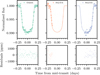 |
Fig. 4 Top: TESS and NGTS detrended photometric observations of TOI-2449 (TESS in green, NGTS in orange and blue) with the common transit model (solid lines). NGTS data are binned at a 10-minute cadence to match the TESS cadence. Bottom: residuals between the transit model and the respective light curve. |
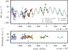 |
Fig. 5 Radial velocity time series with the median model (top panel) and residuals (bottom panel). |
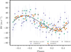 |
Fig. 6 Phase-folded radial velocity plot of TOI-2449 b. |
4.2 Interior modelling of TOI-2449 b
TOI-2449 b is part of the growing sample of transiting warm Jupiters. Assuming a Jupiter-like bond albedo (A=0.343) and full heat redistribution, TOI-2449 b has an equilibrium temperature of  K. The upper and lower bounds were calculated with A=0 and A=0.686, respectively. At this equilibrium temperature, the atmosphere of this planet is not expected to be inflated. Indeed TOI-2449 b receives an insolation flux of 1.107 erg s−1 cm−2, which is lower than the usual threshold for inflation of 2.108 erg s−1 cm−2 observed by Miller & Fortney (2011) and Demory & Seager (2011). This insolation threshold corresponds to an equilibrium temperature of about 1000 K.
In contrast to transiting hot Jupiters, transiting warm Jupiters are ideal for the study of their internal composition. The link between the interior composition and the planetary size is more straightforward because these planets are not subject to inflation mechanisms. The heavy element content is one parameter that can be well constrained by the interior modelling of gas giant planets. For gas giant planets, the majority of the mass is made of hydrogen and helium, and only a small fraction is made of other elements, which we refer to as heavy elements or simply metals. Heavy elements have a large impact on the planetary radius, and increasing the heavy element content leads to smaller radii (e.g. Baraffe et al. 2008; Miller & Fortney 2011).
We used the planetary evolution code completo (Mordasini et al. 2012) to build a grid of interior models for gas giant planets orbiting FGK and M stars. The planets are modelled as a core and an envelope coupled with a semi-grey atmospheric model. The planets have masses ranging from 15 M⊕ to 13 MJup and semi-major axes ranging from 0.1 to 10 au. The core mass can vary from 0 to 10 M⊕ and is made of iron and silicates, with an iron mass fraction of 33%. The H/He envelope is modelled with the H/He equation of state from Chabrier & Debras (2021). The heavier elements are assumed to be homogeneously mixed in the envelope and are modelled as water according to the AQUA equation of state (Haldemann et al. 2020). We did not consider inflation mechanisms, as it is unlikely to affect planets on such wide orbits (e.g. Demory & Seager 2011). The grid of evolution models was then coupled to a Bayesian inference model to retrieve the heavy element content of TOI-2449 b.
In this framework, we used information from the photometric, radial velocity joint fit and the host star analysis to set normal priors on the planetary mass, stellar mass, and stellar age and to fix the semi-major axis to its median value. The prior on the metal fraction of the envelope (Zenv) is a uniform prior between 0 and 0.9. Given the planetary parameters, Zenv, and stellar age, we calculated the corresponding evolution models. We then obtained the distribution of theoretical radii and interior compositions compatible with TOI-2449 b.
We find that TOI-2449 b has an envelope marginally enriched in heavy elements by a fraction  . The core mass is not well constrained by our retrieval (
 )· By adding the mass of heavy elements in the envelope and the core mass, we find that the total heavy element mass is
  . Hence, the total heavy element mass fraction (Mz/Mp) is
  . We estimated the overall stellar metallicity from the iron abundance as follows, Z★ = 0.0142 × 10[Fe//H] (Asplund et al. 2009; Miller & Fortney 2011), and we obtained Z★ = 0.0133 ± 0.0012. The planet metal enrichment of TOI-2449 b is
  . Due to its relatively low planetary mass compared to its radius, the Jupiter-sized planet TOI-2449 b is consistent with no metal enrichment relative to its host star at 1σ. We note that several interior models exist to probe the composition of giant exoplanets (e.g. Müller et al. 2020; Acuña et al. 2024; Sur et al. 2024), and they may lead to differences in the exact derived values of planet metallicity.
Fitted and derived parameters of TOI-2449 b.
5 Discussion
TOI-2449 b joins the small population of well-characterised transiting planets orbiting a bright host star with a relatively long period of 106 days. In Fig. 7, we present TOI-2449 b within the sample of transiting exoplanets taken from the TEPCat catalogue7. We selected exoplanets with planetary masses larger than 0.1 MJ and uncertainty on their planetary mass and radius measurements smaller than 8% and 20%, respectively. While there is a growing sample of well-characterised transiting gas giant planets with orbital periods larger than 10 days, only 23 planets have an orbital period larger than 100 days, and 10 planets transit a bright host star (Vmag < 12). Figure 8 displays only the warm giant planets with an equilibrium temperature below 1000 K. This temperature threshold is commonly used to define the limit below which the planetary atmosphere is usually not inflated. From Fig. 8, we noticed that the warm giant planets do not have planetary radii above 1.2 RJ.
We compared TOI-2449 b with the outputs of the New Generation Planetary Population Synthesis formation and evolution model (Emsenhuber et al. 2021b), which is built on the core accretion paradigm. We used the NG76longshot population based on Emsenhuber et al. (2021a) with a longer integration time of 100 Myr and the inclusion of realistic water phases (see Burn et al. 2024 for details). We observed that synthetic planets close to the mass, radius, and semi-major of TOI-2449 b form in the outer part of the disc between 3 and 6 au. These planets first grow to about 10 M⊕ at their formation location and then migrate inward while accreting large quantities of gas and increasing their total mass. TOI-2449 b contains about 11 M⊕ of metals, a value that is in agreement with the closest synthetic planets in this population. Hence, TOI-2449 b likely formed at a few aus from its host star, then migrated inward while essentially accreting gas to be found at its current location. At this stage, we cannot pinpoint the migration pathway of TOI-2449 b. A measure of the projected spin-orbit angle of the system would help us distinguish between possible migration mechanisms such as disc migration or high-eccentricity migration. The expected Rossiter-McLaughlin signal is about 35 m.s−1 (Eq. (40), Winn 2010). Thanks to the v.sini of the host star, the Rossiter-McLaughlin effect is large and should be easily detectable with high-resolution spectrographs such as HARPS and ESPRESSO. Given the long transit duration of TOI-2449 b, ground-based spectroscopic observations could be performed in two separate visits covering the first and second half of the transit. In the next three years, there are two transit opportunities from Paranal, Chile. The mid transit times in BJD are  (08.Dec.2026 03:10 UTC) and
  (20.Dec.2028 03:27 UTC).
Finally, atmospheric characterisation of such warm and temperate planets would be useful to understanding the link between the well-studied hot Jupiters and the gas giants of the Solar System. We estimated the Transmission Spectrocopy Metric (TSM; Kempton et al. 2018) of TOI-2449 b to be 38. The TSM value is low compared to the values for hot Jupiters. However, for a temperate giant planet, a TSM of around 30 is enough to be considered as one of the best targets to perform transmission spectroscopy (e.g. Kepler-16b, Hord et al. 2024). With an equilibrium temperature of about 400 K and a mass measured with a precision better than 10%, TOI-2449 b is a suitable target for transmission spectrocopy with JWST for the class of temperate giant planets. In Sect. 4.2 we estimated the planetary metal mass fraction Zp using a planetary evolution model. From this metal mass fraction, we could infer the metal abundance ratio Z:H (by number) following Eq. (3) from Thorngren & Fortney (2019). We found a Z:H ratio of  . This value provides an upper limit on the atmospheric metallicity since Zp was derived assuming that the metals in the envelope are homogeneously mixed.
Atmospheric characterisation of temperate gas giants such as TOI-2449 b allows us to build a connected understanding of giant planet populations across the parameter space, combining with dynamical clues such as eccentricity, obliquity, and system architecture preserved in the orbits of these planets to infer the planet formation and migration history (Dawson & Johnson 2018). Particularly notable at these temperatures, CH4 and NH3 are the equilibrium carriers of carbon and nitrogen (Fortney et al. 2020), compared to CO and N2 for hot Jupiters. Notably NH3 only appears in these cooler planets (<500 K), and unlike N2, it can be detected with transmission spectroscopy. This means that the C/N/O ratio can be uniquely measured, which can be more precisely related to the planet’s formation and migration history than the C/O ratio alone (e.g. Piso et al. 2016; Cridland et al. 2020). In Fig. 9, we present synthetic transmission spectra for TOI-2449 b using an equilibrium chemistry model and different metallicities within the range implied by internal structure modelling using petitRADTRANS (Mollière et al. 2019). Simulated observations from the NIRISS/SOSS and NIRSpec/G395M instruments (Batalha et al. 2017) are displayed along the simulated spectra, showing detectable variations, in particular for the CH4 features at 2.2 and 3.3 µm and the NH3 feature at 1.5 and 3 µm.
Furthermore, the atmospheres of temperate gas giants are predicted to host diverse disequilibrium chemistry processes, including condensation of both S8 and H2O (Gao et al. 2017; Mang et al. 2022), photochemical destruction of NH3, production of HCN (Hu 2021; Ohno & Fortney 2023b), and chemical quenching due to vertical mixing (Fortney et al. 2020; Ohno & Fortney 2023a). These processes are dependent on many factors, including the temperature, stellar host, metallicity, and gravity, making it important to have a diverse sample of temperate gas giants for atmospheric characterisation. TOI-2449 b joins TOI-2447 b (Gill et al. 2024), NGTS-30 b (Battley et al. 2024), and TOI-2010 b (Mann et al. 2023) in a cluster of 400–500 K Jupiters around Sun-like hosts, covering a range of masses from 0.5–1.2 MJ and an excellent regime for understanding nitrogen chemistry.
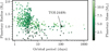 |
Fig. 7 Planetary radius as a function of orbital period colour-coded by the planetary mass for known transiting giant exoplanets. |
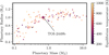 |
Fig. 8 Radius-mass distribution colour-coded by the equilibrium temperature for transiting warm giant exoplanets (Teq < 1000 K). |
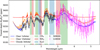 |
Fig. 9 Synthetic transmission spectra of TOI-2449 b from petitRADTRANS (Mollière et al. 2019), assuming equilibrium chemistry and an isothermal atmosphere. We used 1×, 3×, and 10× models with a solar C/O ratio and include a grey cloud deck at 1 mbar for the cloudy model. Simulated flux measurements from NIRISS/SOSS and NIRSpec/G395M instrument are shown as black and pink points. |
6 Conclusions
We report the discovery and characterisation of TOI-2449 b / NGTS-36 b, a 106-day warm giant exoplanet orbiting a G-type star. This planet was first identified as a single transit event in the TESS data. Ground-based photometric follow-up with NGTS and radial velocity follow-up solved the orbital period to 106.144 days, corresponding to a semi-major axis of 0.449 au. The planet has a mass of  MJ and a radius of 1.001±0.0009 RJ and is on a slightly eccentric orbit. We detect an additional 3-year periodic signal in the radial velocity data that is most likely the magnetic activity cycle of the star. TOI-2449 b / NGTS-36 b joins the growing sample of transiting warm Jupiters orbiting relatively bright stars. Further observations of the Rossiter-McLaughlin effect produced by TOI-2449 b / NGTS-36 b and atmospheric characterisation through transmission spectroscopy are achievable and will allow us to learn more about the formation and evolution pathway of this system.
Data availability
The full version of Table 1 is available at the CDS via https://cdsarc.cds.unistra.fr/viz-bin/cat/J/A+A/703/A258.
Acknowledgements
This work has been carried out within the framework of the National Centre of Competence in Research PlanetS supported by the Swiss National Science Foundation (SNSF) under grants 51NF40_182901 and 5INF40_205606. The authors acknowledge the financial support of the SNSF This work is based on data collected under the NGTS project at the ESO Paranal Observatory. The NGTS facility is operated by a consortium institutes with support from the UK Science and Technology Facilities Council (STFC) under projects ST/M001962/1, ST/S002642/1 and ST/W003163/1. The contributions at the University of Warwick by SG, DB, PJW, RGW and DA have been supported by STFC through consolidated grants ST/P000495/1, STT000406/1 and ST/X001121/1. KA acknowledges support from the SNSF under the Post-doc Mobility grant P500PT_230225. ML acknowledges support of the SNSF under grant number PCEFP2194576. This paper made use of data collected by the TESS mission and are publicly available from the Mkulski Archive for Space Telescopes (MAST) operated by the Space Telescope Science Institute (STScI). Funding for the TESS mission is provided by NASA’s Science Mission Directorate. Resources supporting this work were provided by the NASA High-End Computing (HEC) Program through the NASA Advanced Super-computing (NAS) Division at Ames Research Center for the production of the SPOC data products. KAC acknowledges support from the TESS mission via subaward s3449 from MIT. R.B. acknowledges support from FONDECYT Project 1241963 and from ANID – Millennium Science Initiative – ICNI2_009. This work was funded by the Data Observatory Foundation. A.De. acknowledges financial support from the Swiss National Science Foundation (SNSF) for project 200021_200726. A.J. acknowledges support from ANID – Mllennium Science Initiative – ICNI2_009, AIM23-0001 and from FONDECYT project 1210718. M.T.P. acknowledges support from Fondecyt-ANID fellowship no. 3210253 and ASTRON-0037. A.P acknowledges support from the Unidad de Excelencia María de Maeztu CEX2020-001058-M programme and from the Generalitat de Catalunya/CERCA. The results reported herein benefitted from collaborations and/or information exchange within NASA’s Nexus for Exoplanet System Science (NExSS) research coordination network sponsored by NASA’s Science Mission Directorate under Agreement No. 80NSSC21K0593 for the program “Alien Earths”. GV has received support from the European Research Council (ERC) under the European Union s Horizon 2020 research and innovation programme (Grant Agreement No. 947660). Some of the observations in this paper made use of the High-Resolution Imaging instrument Zorro and were obtained under Gemini LLP Proposal Number: GN/S-2021A-LP-105. Zorro was funded by the NASA Exoplanet Exploration Program and built at the NASA Ames Research Center by Steve B. Howell, Nic Scott, Elliott P. Horch, and Emmett Quigley. Zorro was mounted on the Gemini South telescope of the international Gemini Observatory, a program of NSF’s OIR Lab, which is managed by the Association of Universities for Research in Astronomy (AURA) under a cooperative agreement with the National Science Foundation. on behalf of the Gemini partnership: the National Science Foundation (United States), National Research Council (Canada), Agencia Nacional de Investigación y Desarrollo (Chile), Ministerio de Ciencia, Tecnología e Innovación (Argentina), Ministério da Ciência, Tecnologia, Inovações e Comunicações (Brazil), and Korea Astronomy and Space Science Institute (Republic of Korea). C.A.W. would like to acknowledge support from the UK Science and Technology Facilities Council (STFC, grant number ST/X00094X/1). JSJ greatfully acknowledges support by FONDECYT grant 1240738 and from the ANID BASAL project FB210003. The contributions at the Mullard Space Science Laboratory by EMB have been supported by STFC through the consolidated grant ST/W001136/1. TR is supported by an STFC studentship.
References
- Acuña, L., Kreidberg, L., Zhai, M., & Mollière, P. 2024, A&A, 688, A60 [NASA ADS] [CrossRef] [EDP Sciences] [Google Scholar]
- Albrecht, S., Winn, J. N., Johnson, J. A., et al. 2012, ApJ, 757, 18 [NASA ADS] [CrossRef] [Google Scholar]
- Albrecht, S. H., Dawson, R. I., & Winn, J. N. 2022, PASP, 134, 082001 [NASA ADS] [CrossRef] [Google Scholar]
- Aller, A., Lillo-Box, J., Jones, D., Miranda, L. F., & Barceló Forteza, S. 2020, A&A, 635, A128 [NASA ADS] [CrossRef] [EDP Sciences] [Google Scholar]
- Asplund, M., Grevesse, N., Sauval, A. J., & Scott, P. 2009, Annu. Rev. Astron. Astrophys., 47, 481 [CrossRef] [Google Scholar]
- Baraffe, I., Chabrier, G., & Barman, T. 2008, A&A, 482, 315 [NASA ADS] [CrossRef] [EDP Sciences] [Google Scholar]
- Baranne, A., Queloz, D., Mayor, M., et al. 1996, A&A Suppl, 119, 373 [Google Scholar]
- Barnes, S. A. 2010, ApJ, 722, 222 [Google Scholar]
- Baruteau, C., Crida, A., Paardekooper, S. J., et al. 2014, Planet-Disk Interactions and Early Evolution of Planetary Systems (Protostars and Planets VI: University of Arizona Press), 667 [Google Scholar]
- Batalha, N. E., Mandell, A., Pontoppidan, K., et al. 2017, PASP, 129, 064501 [Google Scholar]
- Battley, M. P., Collins, K. A., Ulmer-Moll, S., et al. 2024, A&A, 686, A230 [NASA ADS] [CrossRef] [EDP Sciences] [Google Scholar]
- Blackwell, D. E., & Shallis, M. J. 1977, MNRAS, 180, 177 [NASA ADS] [CrossRef] [Google Scholar]
- Bodenheimer, P., Hubickyj, O., & Lissauer, J. J. 2000, Icarus, 143, 2 [Google Scholar]
- Bonfanti, A., Ortolani, S., Piotto, G., & Nascimbeni, V. 2015, A&A, 575, A18 [NASA ADS] [CrossRef] [EDP Sciences] [Google Scholar]
- Bonfanti, A., Ortolani, S., & Nascimbeni, V. 2016, A&A, 585, A5 [NASA ADS] [CrossRef] [EDP Sciences] [Google Scholar]
- Bonfanti, A., Delrez, L., Hooton, M. J., et al. 2021, A&A, 646, A157 [EDP Sciences] [Google Scholar]
- Brahm, R., Jordan, A., & Espinoza, N. 2017, PASP, 129, 034002 [NASA ADS] [CrossRef] [Google Scholar]
- Brahm, R., Ulmer-Moll, S., Hobson, M. J., et al. 2023, AJ, 165, 227 [NASA ADS] [CrossRef] [Google Scholar]
- Bryant, E. M., Bayliss, D., McCormac, J., et al. 2020, MNRAS, 494, 5872 [Google Scholar]
- Burn, R., Mordasini, C., Mishra, L., et al. 2024, Nat. Astron., 8, 463 [Google Scholar]
- Castelli, F., & Kurucz, R. L. 2003, in IAU Symposium, 210, Modelling of Stellar Atmospheres, eds. N. Piskunov, W. W. Weiss, & D. F. Gray, A20 [NASA ADS] [Google Scholar]
- Chabrier, G., & Debras, F. 2021, ApJ, 917, 4 [NASA ADS] [CrossRef] [Google Scholar]
- Ciardi, D. R., Beichman, C. A., Horch, E. P., & Howell, S. B. 2015, ApJ, 805, 16 [NASA ADS] [CrossRef] [Google Scholar]
- Cooke, B. F., Pollacco, D., & Bayliss, D. 2019, A&A, 631, A83 [NASA ADS] [CrossRef] [EDP Sciences] [Google Scholar]
- Cridland, A. J., van Dishoeck, E. F., Alessi, M., & Pudritz, R. E. 2020, A&A, 642, A229 [NASA ADS] [CrossRef] [EDP Sciences] [Google Scholar]
- Dalba, P. A., Kane, S. R., Dragomir, D., et al. 2022, AJ, 163, 61 [NASA ADS] [CrossRef] [Google Scholar]
- Dawson, R. I., & Johnson, J. A. 2018, ARA&A, 56, 175 [Google Scholar]
- Delisle, J. B., Hara, N., & Ségransan, D. 2020, A&A, 635, A83 [NASA ADS] [CrossRef] [EDP Sciences] [Google Scholar]
- Demory, B.-O., & Seager, S. 2011, ApJS, 197, 12 [NASA ADS] [CrossRef] [Google Scholar]
- Eastman, J., Gaudi, B. S., & Agol, E. 2013, PASP, 125, 83 [Google Scholar]
- Eberhardt, J., Hobson, M. J., Henning, T., et al. 2023, AJ, 166, 271 [NASA ADS] [CrossRef] [Google Scholar]
- Emsenhuber, A., Mordasini, C., Burn, R., et al. 2021a, A&A, 656, A69 [NASA ADS] [CrossRef] [EDP Sciences] [Google Scholar]
- Emsenhuber, A., Mordasini, C., Burn, R., et al. 2021b, A&A, 656, A70 [NASA ADS] [CrossRef] [EDP Sciences] [Google Scholar]
- Espinoza, N., & Jordán, A. 2015, MNRAS, 450, 1879 [Google Scholar]
- Espinoza, N., Kossakowski, D., & Brahm, R. 2019, MNRAS, 490, 2262 [Google Scholar]
- Faria, J. P., Santos, N. C., Figueira, P., & Brewer, B. J. 2018, J. Open Source Softw., 3, 487 [NASA ADS] [CrossRef] [Google Scholar]
- Feroz, F., Balan, S. T., & Hobson, M. P. 2011, MNRAS, 415, 3462 [Google Scholar]
- Fortney, J. J., Visscher, C., Marley, M. S., et al. 2020, AJ, 160, 288 [NASA ADS] [CrossRef] [Google Scholar]
- Fulton, B. J., Petigura, E. A., Blunt, S., & Sinukoff, E. 2018, PASP, 130, 044504 [Google Scholar]
- Furlan, E., & Howell, S. B. 2017, AJ, 154, 66 [NASA ADS] [CrossRef] [Google Scholar]
- Furlan, E., & Howell, S. B. 2020, ApJ, 898, 47 [NASA ADS] [CrossRef] [Google Scholar]
- Gaia Collaboration (Brown, A. G. A., et al.) 2021, A&A, 649, A1 [NASA ADS] [CrossRef] [EDP Sciences] [Google Scholar]
- Gaia Collaboration (Vallenari, A., et al.) 2023, A&A, 674, A1 [NASA ADS] [CrossRef] [EDP Sciences] [Google Scholar]
- Gao, P., Marley, M. S., Zahnle, K., Robinson, T. D., & Lewis, N. K. 2017, AJ, 153, 139 [NASA ADS] [CrossRef] [Google Scholar]
- Gibson, N. P. 2014, MNRAS, 445, 3401 [NASA ADS] [CrossRef] [Google Scholar]
- Gill, S., Wheatley, P. J., Cooke, B. F., et al. 2020, ApJ, 898, L11 [Google Scholar]
- Gill, S., Bayliss, D., Ulmer-Moll, S., et al. 2024, MNRAS, 532, 1444 [Google Scholar]
- Goldreich, P., & Tremaine, S. 1980, ApJ, 241, 425 [Google Scholar]
- Gomes da Silva, J., Bensabat, A., Monteiro, T., & Santos, N. C. 2022, A&A, 668, A174 [NASA ADS] [CrossRef] [EDP Sciences] [Google Scholar]
- Gray, D. F. 2005, The Observation and Analysis of Stellar Photospheres [Google Scholar]
- Haldemann, J., Alibert, Y., Mordasini, C., & Benz, W. 2020, A&A, 643, A105 [NASA ADS] [CrossRef] [EDP Sciences] [Google Scholar]
- Hobson, M. J., Brahm, R., Jordan, A., et al. 2021, AJ, 161, 235 [NASA ADS] [CrossRef] [Google Scholar]
- Høg, E., Fabricius, C., Makarov, V. V., et al. 2000, A&A, 355, L27 [Google Scholar]
- Hord, B. J., Kempton, E. M. R., Evans-Soma, T. M., et al. 2024, AJ, 167, 233 [NASA ADS] [CrossRef] [Google Scholar]
- Howell, S. B., Everett, M. E., Sherry, W., Horch, E., & Ciardi, D. R. 2011, AJ, 142, 19 [Google Scholar]
- Howell, S. B., Scott, N. J., Matson, R. A., et al. 2021, Front. Astron. Space Sci., 8, 10 [NASA ADS] [Google Scholar]
- Hu, R. 2021, ApJ, 921, 27 [NASA ADS] [CrossRef] [Google Scholar]
- Huang, C. X., Vanderburg, A., Pál, A., et al. 2020a, RNAAS, 4, 204 [Google Scholar]
- Huang, C. X., Vanderburg, A., Pál, A., et al. 2020b, RNAAS, 4, 206 [NASA ADS] [Google Scholar]
- Husser, T.-O., Berg, S. W.-v., Dreizler, S., et al. 2013, A&A, 553, A6 [NASA ADS] [CrossRef] [EDP Sciences] [Google Scholar]
- Isaacson, H., Howard, A. W., Fulton, B., et al. 2024, The California Legacy Survey V. Chromospheric Activity Cycles in Main Sequence Stars [Google Scholar]
- Jenkins, J. M., Twicken, J. D., McCauliff, S., et al. 2016, SPIE, 9913, 99133E [NASA ADS] [Google Scholar]
- Kaufer, A., Stahl, O., Tubbesing, S., et al. 1999, The Messenger, 95, 8 [Google Scholar]
- Kempton, E. M. R., Bean, J. L., Louie, D. R., et al. 2018, PASP, 130, 114401 [Google Scholar]
- Kipping, D. M. 2013, MNRAS, 435, 2152 [Google Scholar]
- Kong, Z., Johansen, A., Lambrechts, M., Jiang, J. H., & Zhu, Z.-H. 2024, A&A, 687, A121 [NASA ADS] [CrossRef] [EDP Sciences] [Google Scholar]
- Kreidberg, L. 2015, PASP, 127, 1161 [Google Scholar]
- Kurucz, R. L. 1979, ApJS, 40, 1 [NASA ADS] [CrossRef] [Google Scholar]
- Kurucz, R. L. 1993, SYNTHE spectrum synthesis programs and line data [Google Scholar]
- Levison, H. F., & Agnor, C. 2003, AJ, 125, 2692 [NASA ADS] [CrossRef] [Google Scholar]
- Lin, D. N. C., Bodenheimer, P., & Richardson, D. C. 1996, Nature, 380, 606 [Google Scholar]
- Lindegren, L., Bastian, U., Biermann, M., et al. 2021, A&A, 649, A4 [EDP Sciences] [Google Scholar]
- Livingston, W., Wallace, L., White, O. R., & Giampapa, M. S. 2007, ApJ, 657, 1137 [CrossRef] [Google Scholar]
- Mang, J., Gao, P., Hood, C. E., et al. 2022, ApJ, 927, 184 [NASA ADS] [CrossRef] [Google Scholar]
- Mann, C. R., Dalba, P. A., Lafrenière, D., et al. 2023, AJ, 166, 239 [CrossRef] [Google Scholar]
- Marigo, P., Girardi, L., Bressan, A., et al. 2017, ApJ, 835, 77 [Google Scholar]
- Matson, R. A., Howell, S. B., Horch, E. P., & Everett, M. E. 2018, AJ, 156, 31 [NASA ADS] [CrossRef] [Google Scholar]
- Mayor, M., & Queloz, D. 1995, Nature, 378, 355 [Google Scholar]
- Mayor, M., Pepe, F., Queloz, D., et al. 2003, The Messenger, 114, 20 [NASA ADS] [Google Scholar]
- Miller, N., & Fortney, J. J. 2011, ApJ, 736, L29 [NASA ADS] [CrossRef] [Google Scholar]
- Mollière, P., Wardenier, J., Van Boekel, R., et al. 2019, A&A, 627, A67 [NASA ADS] [CrossRef] [EDP Sciences] [Google Scholar]
- Mordasini, C., Alibert, Y., Klahr, H., & Henning, T. 2012, A&A, 547, A111 [NASA ADS] [CrossRef] [EDP Sciences] [Google Scholar]
- Mordasini, C., & Burn, R. 2024, Rev. Mineral. Geochem., 90, 55 [Google Scholar]
- Müller, S., Ben-Yami, M., & Helled, R. 2020, ApJ, 903, 147 [Google Scholar]
- Noyes, R. W., Hartmann, L. W., Baliunas, S. L., Duncan, D. K., & Vaughan, A. H. 1984, ApJ, 279, 763 [Google Scholar]
- O’Brien, S. M., Bayliss, D., Osborn, J., et al. 2021, MNRAS, 509, 6111 [Google Scholar]
- Ohno, K., & Fortney, J. J. 2023a, ApJ, 946, 18 [NASA ADS] [CrossRef] [Google Scholar]
- Ohno, K., & Fortney, J. J. 2023b, ApJ, 956, 125 [CrossRef] [Google Scholar]
- Paredes, L. A., Henry, T. J., Quinn, S. N., et al. 2021, AJ, 162, 176 [NASA ADS] [CrossRef] [Google Scholar]
- Pepe, F., Mayor, M., Rupprecht, G., et al. 2002, The Messenger, 110, 9 [NASA ADS] [Google Scholar]
- Piso, A.-M. A., Pegues, J., & Öberg, K. I. 2016, ApJ, 833, 203 [Google Scholar]
- Queloz, D., Henry, G. W., Sivan, J. P., et al. 2001a, A&A, 379, 279 [NASA ADS] [CrossRef] [EDP Sciences] [Google Scholar]
- Queloz, D., Mayor, M., Udry, S., et al. 2001b, The Messenger, 105, 1 [NASA ADS] [Google Scholar]
- Rasio, F. A., & Ford, E. B. 1996, Science, 274, 954 [Google Scholar]
- Ricker, G. R., Winn, J. N., Vanderspek, R., et al. 2015, J. Astron. Telesc. Instrum. Syst., 1, 014003 [Google Scholar]
- Rodel, T., Bayliss, D., Gill, S., & Hawthorn, F. 2024, MNRAS, 529, 715 [Google Scholar]
- Salmon, S. J. A. J., Van Grootel, V., Buldgen, G., Dupret, M. A., & Eggenberger, P. 2021, A&A, 646, A7 [NASA ADS] [CrossRef] [EDP Sciences] [Google Scholar]
- Santos, N. C., Sousa, S. G., Mortier, A., et al. 2013, A&A, 556, A150 [NASA ADS] [CrossRef] [EDP Sciences] [Google Scholar]
- Schanche, N., Hébrard, G., Collier Cameron, A., et al. 2020, MNRAS, 499, 428 [NASA ADS] [CrossRef] [Google Scholar]
- Schlecker, M., Kossakowski, D., Brahm, R., et al. 2020, AJ, 160, 275 [Google Scholar]
- Scott, N. J., Howell, S. B., Gnilka, C. L., et al. 2021, Front. Astron. Space Sci., 8, 138 [NASA ADS] [CrossRef] [Google Scholar]
- Scuflaire, R., Théado, S., Montalbán, J., et al. 2008, Ap&SS, 316, 83 [Google Scholar]
- Ségransan, D., Udry, S., Mayor, M., et al. 2010, A&A, 511, A45 [NASA ADS] [CrossRef] [EDP Sciences] [Google Scholar]
- Sgro, L. A., Dalba, P. A., Esposito, T. M., et al. 2024, AJ, 168, 26 [Google Scholar]
- Skrutskie, M. F., Cutri, R. M., Stiening, R., et al. 2006, AJ, 131, 1163 [NASA ADS] [CrossRef] [Google Scholar]
- Smith, J. C., Stumpe, M. C., Van Cleve, J. E., et al. 2012, PASP, 124, 1000 [Google Scholar]
- Sneden, C. A. 1973, PhD thesis, The University of Texas at Austin [Google Scholar]
- Sousa, S. G., Santos, N. C., Israelian, G., Mayor, M., & Monteiro, M. J. P. F. G. 2007, A&A, 469, 783 [NASA ADS] [CrossRef] [EDP Sciences] [Google Scholar]
- Sousa, S. G., Santos, N. C., Mayor, M., et al. 2008, A&A, 487, 373 [NASA ADS] [CrossRef] [EDP Sciences] [Google Scholar]
- Sousa, S. G. 2014, ARES + MOOG: A Practical Overview of an Equivalent Width (EW) Method to Derive Stellar Parameters, 297 [Google Scholar]
- Sousa, S. G., Santos, N. C., Adibekyan, V., Delgado-Mena, E., & Israelian, G. 2015, A&A, 577, A67 [NASA ADS] [CrossRef] [EDP Sciences] [Google Scholar]
- Sousa, S. G., Adibekyan, V., Delgado-Mena, E., et al. 2021, A&A, 656, A53 [NASA ADS] [CrossRef] [EDP Sciences] [Google Scholar]
- Speagle, J. S. 2019, A Conceptual Introduction to Markov Chain Monte Carlo Methods [Google Scholar]
- Stumpe, M. C., Smith, J. C., Van Cleve, J. E., et al. 2012, PASP, 124, 985 [Google Scholar]
- Stumpe, M. C., Smith, J. C., Catanzarite, J. H., et al. 2014, PASP, 126, 100 [Google Scholar]
- Suárez Mascareño, A., Rebolo, R., & González Hernández, J. I. 2016, A&A, 595, A12 [Google Scholar]
- Sur, A., Su, Y., Tejada Arevalo, R., Chen, Y.-X., & Burrows, A. 2024, ApJ, 971, 104 [Google Scholar]
- Thorngren, D., & Fortney, J. J. 2019, ApJ, 874, L31 [Google Scholar]
- Tokovinin, A. 2018, PASP, 130, 035002 [Google Scholar]
- Tokovinin, A., Fischer, D. A., Bonati, M., et al. 2013, PASP, 125, 1336 [NASA ADS] [CrossRef] [Google Scholar]
- Ulmer-Moll, S., Lendl, M., Gill, S., et al. 2022, A&A, 666, A46 [NASA ADS] [CrossRef] [EDP Sciences] [Google Scholar]
- Ulmer-Moll, S., Osborn, H. P., Tuson, A., et al. 2023, A&A, 674, A43 [NASA ADS] [CrossRef] [EDP Sciences] [Google Scholar]
- Villanueva, Jr., S., Dragomir, D., & Gaudi, B. S. 2019, AJ, 157, 84 [NASA ADS] [CrossRef] [Google Scholar]
- Wang, X.-Y., Rice, M., Wang, S., et al. 2024, ApJ, 973, L21 [Google Scholar]
- Wheatley, P. J., West, R. G., Goad, M. R., et al. 2018, MNRAS, 475, 4476 [Google Scholar]
- Winn, J. N. 2010, Transits and Occultations [Google Scholar]
- Wright, E. L., Eisenhardt, P. R. M., Mainzer, A. K., et al. 2010, AJ, 140, 1868 [Google Scholar]
- Ziegler, C., Tokovinin, A., Briceño, C., et al. 2020, AJ, 159, 19 [Google Scholar]
NASA exoplanet archive queried on April, 15, 2025, for planets with masses larger than 0.1 MJ.
mast.stsci.edu
eso.org/public/teles-instr/lasilla/swiss
The last version, ARES v2, can be downloaded at https://github.com/sousasag/ARES
PA dova and TRieste Stellar Evolutionary Code: http://stev.oapd.inaf.it/cgi-bin/cmd
Appendix A TESS target pixel file
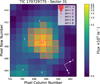 |
Fig. A.1 TESS target pixel file of TOI-2449 with its aperture for the sector 31 plotted with the Gaia EDR3 sources. |
Appendix B NGTS observations
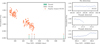 |
Fig. B.1 NGTS flux time series of TOI-2449. Left panel: Nightly binned NGTS data from January 2021 to November 2022 (orange dots). Right panel: Example of NGTS observations (blue dots) during a clear night with no detection (binned to 5 minutes; top), a clear night with a transit detection (binned to 10 minutes; middle and bottom). |
Appendix C Imaging data
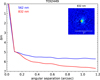 |
Fig. C.1 Speckle imaging contrast curves (5 σ) in both filters as a function of the angular separation out to 1.2 arcsec from TOI-2449. The inset shows the speckle reconstructed 832 nm image with a 1 arcsec scale bar. |
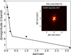 |
Fig. C.2 Detection sensitivity (5 σ) and speckle auto-correlation functions from the SOAR observation of TOI-2449. |
Appendix D Radial velocity modelling priors
Priors for the first radial velocity fit with a maximum of three planets.
Appendix E Radial velocity fit with a GP
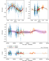 |
Fig. E.1 Top: Radial velocity phase-folded plot of TOI-2449 b (right) and the 3-year activity cycle modelled as a sinusoid (left) for the maximum likelihood solution. Middle: Radial velocity dataset with the corresponding GP model (black). Bottom: Radial velocity residuals. |
Appendix F Joint modelling priors
Prior for the joint modelling of photometric and radial velocity data.
Appendix G TESS observations
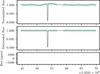 |
Fig. G.1 TESS photometric observations (green dots) with the median transit model (black line). Top: PDCSAP TESS light curves. Middle: Detrended TESS light curves. Bottom: Residuals between the median model and the TESS light curve. |
Appendix H Joint modelling posterior distributions
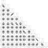 |
Fig. H.1 Posterior distributions of fitted parameters for TOI-2449 b along with the stellar density (ρS) and radial velocity semi-amplitude (KTR). The 3-year RV variation is parametrized with period2, T02, and K2. |
All Tables
All Figures
|
Fig. 1 Radial velocities of TOI-2449. Top: radial velocity data spanning 1136 days (CHIRON, blue; CORALIE, green; FEROS, grey; HARPS, orange). Bottom: generalised Lomb-Scargle periodogram of the radial velocities. The black line marks the 1% false alarm probability. |
| In the text | |
|
Fig. 2 Generalised Lomb–Scargle periodogram of the radial velocities, the radial velocity residuals after joint modelling (see Sect. 3.3), FWHM of the CCF, and Hα indicator. Vertical lines highlight the relevant periods (red: stellar rotation; green: significant signals). The grey line marks the 1 % false alarm probability. |
| In the text | |
|
Fig. 3 Posterior distribution of the orbital period for a model with up to three planets (blue histogram). The prior on the orbital period is identical for the three planets and shown in grey. The ESS is equal to 22 790 samples. |
| In the text | |
|
Fig. 4 Top: TESS and NGTS detrended photometric observations of TOI-2449 (TESS in green, NGTS in orange and blue) with the common transit model (solid lines). NGTS data are binned at a 10-minute cadence to match the TESS cadence. Bottom: residuals between the transit model and the respective light curve. |
| In the text | |
|
Fig. 5 Radial velocity time series with the median model (top panel) and residuals (bottom panel). |
| In the text | |
|
Fig. 6 Phase-folded radial velocity plot of TOI-2449 b. |
| In the text | |
|
Fig. 7 Planetary radius as a function of orbital period colour-coded by the planetary mass for known transiting giant exoplanets. |
| In the text | |
|
Fig. 8 Radius-mass distribution colour-coded by the equilibrium temperature for transiting warm giant exoplanets (Teq < 1000 K). |
| In the text | |
|
Fig. 9 Synthetic transmission spectra of TOI-2449 b from petitRADTRANS (Mollière et al. 2019), assuming equilibrium chemistry and an isothermal atmosphere. We used 1×, 3×, and 10× models with a solar C/O ratio and include a grey cloud deck at 1 mbar for the cloudy model. Simulated flux measurements from NIRISS/SOSS and NIRSpec/G395M instrument are shown as black and pink points. |
| In the text | |
|
Fig. A.1 TESS target pixel file of TOI-2449 with its aperture for the sector 31 plotted with the Gaia EDR3 sources. |
| In the text | |
|
Fig. B.1 NGTS flux time series of TOI-2449. Left panel: Nightly binned NGTS data from January 2021 to November 2022 (orange dots). Right panel: Example of NGTS observations (blue dots) during a clear night with no detection (binned to 5 minutes; top), a clear night with a transit detection (binned to 10 minutes; middle and bottom). |
| In the text | |
|
Fig. C.1 Speckle imaging contrast curves (5 σ) in both filters as a function of the angular separation out to 1.2 arcsec from TOI-2449. The inset shows the speckle reconstructed 832 nm image with a 1 arcsec scale bar. |
| In the text | |
|
Fig. C.2 Detection sensitivity (5 σ) and speckle auto-correlation functions from the SOAR observation of TOI-2449. |
| In the text | |
|
Fig. E.1 Top: Radial velocity phase-folded plot of TOI-2449 b (right) and the 3-year activity cycle modelled as a sinusoid (left) for the maximum likelihood solution. Middle: Radial velocity dataset with the corresponding GP model (black). Bottom: Radial velocity residuals. |
| In the text | |
|
Fig. G.1 TESS photometric observations (green dots) with the median transit model (black line). Top: PDCSAP TESS light curves. Middle: Detrended TESS light curves. Bottom: Residuals between the median model and the TESS light curve. |
| In the text | |
|
Fig. H.1 Posterior distributions of fitted parameters for TOI-2449 b along with the stellar density (ρS) and radial velocity semi-amplitude (KTR). The 3-year RV variation is parametrized with period2, T02, and K2. |
| In the text | |
Current usage metrics show cumulative count of Article Views (full-text article views including HTML views, PDF and ePub downloads, according to the available data) and Abstracts Views on Vision4Press platform.
Data correspond to usage on the plateform after 2015. The current usage metrics is available 48-96 hours after online publication and is updated daily on week days.
Initial download of the metrics may take a while.