| Issue |
A&A
Volume 703, November 2025
|
|
|---|---|---|
| Article Number | A150 | |
| Number of page(s) | 7 | |
| Section | Extragalactic astronomy | |
| DOI | https://doi.org/10.1051/0004-6361/202555323 | |
| Published online | 14 November 2025 | |
Disentangling two spectral components in the X-ray emission of the blazar 1ES 0229+200
1
Institute of Nuclear Physics, Polish Academy of Sciences, ul. Radzikowskiego 152, 31-342 Kraków, Poland
2
Landessternwarte, Universität Heidelberg, Königstuhl 12, D 69117 Heidelberg, Germany
3
Academic Computer Centre CYFRONET of the AGH University of Krakow, Nawojki 11, 30-950 Kraków P.O. Box 6, Poland
⋆ Corresponding author: This email address is being protected from spambots. You need JavaScript enabled to view it.
Received:
28
April
2025
Accepted:
10
September
2025
Abstract
X-ray observations are essential to achieve a deeper understanding of the broadband emission mechanism in blazars. Here, we present a long-term spectral and temporal analysis of X-ray and optical observations of 1ES 0229+200 collected with the Neil Gehrels Swift Observatory from 2008 to 2024, complemented by hard X-ray observations from the Nuclear Spectroscopic Telescope Array (NuSTAR). The blazar 1ES 0229+200 is a high-frequency, peaked BL Lac object, known for its exceptionally hard very high-energy (VHE) γ-ray spectrum extending up to 10 TeV. In August 2021, NuSTAR observed the source in a low X-ray state, revealing a concave spectral shape with a distinct upturn around 25 keV. This feature contrasts with previous observations performed with NuSTAR and Swift-BAT, which showed no such spectral upturn. Previous observations of 1ES 0229+200 and broadband SED (spectral energy distribution) modelling suggest that its X-ray emission extends beyond 100 keV without a significant cutoff. The newly detected spectral upturn may indicate a transition between the synchrotron and inverse Compton components or could be linked to photohadronic processes involving high-energy neutrinos. We discuss the implications of this finding in the context of blazar spectral energy distributions, particularly the potential existence of a third SED bump in the kiloelectronvolt to megaelectronvolt range. The observed spectral features support the hypothesis that 1ES 0229+200 could be a source of high-energy neutrino emission.
Key words: galaxies: active / BL Lacertae objects: individual: 1ES 0229+200 / galaxies: jets / X-rays: galaxies
© The Authors 2025
 Open Access article, published by EDP Sciences, under the terms of the Creative Commons Attribution License (https://creativecommons.org/licenses/by/4.0), which permits unrestricted use, distribution, and reproduction in any medium, provided the original work is properly cited.
This article is published in open access under the Subscribe to Open model. This email address is being protected from spambots. You need JavaScript enabled to view it. to support open access publication.
1. Introduction
Blazars are radio-loud active galactic nuclei characterised by relativistically beamed, non-thermal jet emission pointing towards the observer’s line of sight (Begelman et al. 1984; Urry et al. 2000). These objects exhibit strong variability in both the spectral and temporal domains, with changes observable across all energy bands on timescales as short as days or even hours (e.g. Wagner & Witzel 1995). The broadband electromagnetic spectra of blazars feature two distinct peaks in the ν – νFν representation, one spanning from radio to optical-X-ray frequencies, and the other peaking at high-energy γ rays. The low-energy peak in the SED (spectral energy distribution) is usually explained by synchrotron radiation of relativistic electrons from the jet, whereas the high-energy component can be explained in leptonic and/or hadronic explanations (see e.g. Marscher 1980; Böttcher et al. 2013).
Lepto-hadronic models propose that hadrons are accelerated alongside leptons, resulting in processes such as pion production and synchrotron radiation from secondary particles (Mannheim 1993). A natural outcome of these secondary interactions is the production of neutrinos. In such scenarios, neutrinos can be generated within optically thick regions, where the suppression of high-energy γ-ray emission (E ∼ GeV–TeV) due to γγ absorption may lead to an enhanced flux in the soft-to-hard X-ray band (Petropoulou et al. 2015, 2020; Murase et al. 2016; Reimer et al. 2019; Oikonomou et al. 2021). X-ray observations thus provide key diagnostics of the emission processes at play and can contribute to the distinguishing between leptonic and hadronic origin models (e.g. Zhang et al. 2019).
Blazars are classified in two subgroups: flat-spectrum radio quasars (FSRQs) and BL Lacertae (BL Lac) type objects. BL Lac objects can further be categorized based on the location of the low-energy peak in their SED into high-energy-peaked (HBL), intermediate-energy-peaked (IBL), and low-energy-peaked (LBL) blazars (e.g. Padovani & Giommi 1995; Abdo et al. 2010). For LBL-type blazars the synchrotron bump is located in the infrared regime (νs ≲ 1014 Hz), for IBL-type blazars in the optical-UV range (1014 Hz < νs ≲ 1015 Hz), while for HBL blazars up to the X-ray domain (νs > 1015 Hz; Abdo et al. 2010).
As a result of these characteristics, the position of the X-ray spectrum within the broadband SED varies across the BL Lac subclasses. In HBL blazars, the X-ray spectrum generally covers the synchrotron domain, whereas in LBL blazars, it is located within the inverse Compton region of the SED. Interestingly, in some IBL blazars, the X-ray spectrum spans both the synchrotron and inverse Compton components, leading to a noticeable spectral upturn in the X-ray energy range visible for this type of blazar (see Wierzcholska & Wagner 2016, and references therein).
The high-frequency peaked BL Lac object 1ES 0229+200 located at a redshift of z = 0.1396 (Woo et al. 2005) is frequently observed at different energy wavelengths (see e.g. Rector et al. 2003; Giommi et al. 1995; Kaufmann et al. 2011; Wierzcholska et al. 2015; Cologna et al. 2015; Ehlert et al. 2023). The SED of 1ES 0229+200 is reported to ranging even above 100 keV without any significant cut-off (Kaufmann et al. 2011), classifying the blazar as an extreme HBL-type source. In the X-ray frequencies, it was discovered by the Einstein IPC Slew Survey (Elvis et al. 1992), and since then it has been the target of numerous X-ray observational campaigns.
NuSTAR has clearly detected 1ES 0229+200 up to energies of ∼50 keV (Furniss et al. 2015; Sahakyan 2021). The X-ray spectrum in the NuSTAR band is characterized by a very hard photon index, typically in the range Γ ∼ 1.5 − 2.0, consistent with the continuation of the synchrotron component to very high energies. This hard X-ray tail is detected even during low flux states, suggesting a persistent population of ultra-relativistic electrons (Sahakyan 2021).
The broadband spectral-energy-distribution modelling supports the interpretation that the X-ray emission in the NuSTAR band arises from synchrotron radiation of highly energetic electrons. In particular, the extension of the synchrotron spectrum to hard X-rays, without any clear indication of a cut-off within the NuSTAR band, places strong constraints on the maximum energy of accelerated electrons (Furniss et al. 2015). These electrons can also be responsible for the inverse Compton emission observed in the TeV regime, making NuSTAR observations an essential component in one-zone synchrotron-self-Compton (SSC) modelling (Aliu et al. 2014).
Moreover, the hard TeV spectrum observed by H.E.S.S. and VERITAS (Aharonian et al. 2007; Aliu et al. 2014), in combination with the hard X-ray data from NuSTAR, has been used to place lower limits on the strength of the intergalactic magnetic field (IGMF; Tavecchio & Ghisellini 2010). These studies rely on the assumption of minimal variability and a hard intrinsic TeV spectrum, both of which are supported by the X-ray observations.
Despite being a bright optical and X-ray source, it is a rather faint radio and γ-ray emitter. In the TeV γ rays, it was detected with the H.E.S.S. telescopes in 2006 (Aharonian et al. 2007). Contrary to the X-ray variability, in the very high-energy gamma rays 1ES 0229+200 exhibit hints of variability (see e.g. Aliu et al. 2014).
In this paper, we focus on the long-term X-ray variability of 1ES 0229+200 using data collected with Swift-XRT. We also report on the low-X-ray-state observations collected with NuSTAR. The paper is organised as follows: Sect. 2 describes data used and analysis techniques; results are given in Sect. 3; while the studies are summarised in Sect. 4.
2. Data analysis
2.1. NuSTAR observations
NuSTAR is a Small Explorer satellite dedicated to X-ray observations in the energy regime of 3–79 keV (Harrison et al. 2013). Only 1ES 0229+200 was observed with NuSTAR three times in 2013 and three times in 2021. The set of 2013 was already discussed by e.g. Pandey et al. (2017), Bhatta et al. (2018), Wierzcholska & Wagner (2020). Here, we focus on three observations taken in August 2021, corresponding to the ObsIDs of 10702609002, 10702609004, and 10702609006.
For all three observations, the raw data were processed with the NuSTAR Data Analysis Software package released within HEASoft (v. 6.33.2). For the analysis, a source region was selected within a circle centred on the blazar. The same-size circular region, but located in a different position on a map, was used in order to define background area. Different positions of the background region were used in order to check whether the background selection affects the analysis results. In the analysis performed, only channels corresponding to the energy range of 3–40 keV were selected. All spectra, along with the ancillary and response files, were generated using the nuproducts task for point-like sources. All spectra were binned using grppha to have at least 20 counts per channel. For each ObsID, spectra were fitted using the power-law log-parabola (curved power-law). The models used are defined as follows:
-
a single power law:
 (1)
(1)with the spectral index γ and the normalization Np;
-
a log-parabola:
 (2)
(2)with the normalisation Nl, the spectral index α, and the curvature parameter β;
-
a broken power law:
 (3)
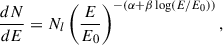
(3)with the normalisation Nb, the spectral indices Γ1 and Γ2, and the break energy Eb.
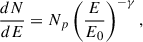
In the case of power-law and log-parabola models, the scale energy E0 is fixed at 1 keV.
A summary of all NuSTAR observations taken both in 2013 and 2021 as well IDs of the corresponding IDs of simultaneous Swift-XRT observations are given in Table 1. Table 2 includes results of the spectral fitting of the NuSTAR data with three spectral models.
NuSTAR observations of 1ES 0229+200 and simultaneous Swift-XRT ones.
Spectral fits parameters for the NuSTAR observations of 1ES 0229+200.
2.2. Swift-XRT and Swift-UVOT observations
The observations collected in the period of 2008-2024, corresponding to the ObsIDs of 00031249001-00016432016, were analysed with the HEASoft package (v. 6.33.2). All events were cleaned and calibrated using the xrtpipeline task, and all PC- and WT-mode data in the energy range of 0.3–10 keV were used. For the spectral fitting, the data were grouped with the grappha task in order to have a minimum of 20 counts per bin. The spectra were fitted with the single-power-law model together with the Galactic-column-density value of 1.16 ⋅ 1021 cm−2 (Willingale et al. 2013) using the XSPEC software (Arnaud 1996). For all fits, the NH was frozen as a fixed parameter. The results of the spectral fitting are listed in Table 3.
Spectral fits parameters for Swift-XRT observations of 1ES 0229+200.
Simultaneously, the blazar was observed with the UVOT instrument on board Swift in the U (345 nm), B (439 nm), and V (544 nm) filters. For all observations corresponding to the ObsIDs of 00031249001-00016432016, the instrumental magnitudes were calculated using uvotsource including all photons from a circular region with a radius of 5”. The background was determined from a circular region with a radius of 10” near the source region that is not contaminated with signal from nearby sources. The flux-conversion factors are provided by Poole et al. (2008). All data were corrected for or the dust absorption using the reddening E(B − V) = 0.1185 mag as provided by Schlafly & Finkbeiner (2011) and the ratios of extinction to reddening, Aλ/E(B − V), for each filter provided by Giommi et al. (2006) are used.
We note here that for the last epoch of the XRT observations, the corresponding UVOT points are not available. During this epoch, a technical issue of the instrument and an increase in noise in one of the three onboard gyroscopes were reported. The UV and optical observations for this period cannot be analysed (for details, see Cenko 2023).
In addition, Table 3 includes the spectral fit parameters for a power-law fit of the Swift-XRT observations simultaneous to six NuSTAR observations. In the case of the NuSTAR observation with ObsID of 10702609002, two Swift-XRT observations are merged.
3. Results
3.1. Characterisation of the variability
The long-term light curve of 1ES 0229+200 spanning from 2008 to 2024, which includes both optical and X-ray observations, is shown in Fig. 1. The figure is divided into three panels that display the variability in optical fluxes, X-ray flux, and the photon index, the latter two derived from power-law spectral fits within the 0.3–10 keV energy band. The X-ray data reveal significant flux variability, with changes of a factor of four, accompanied by shifts in the photon index ranging between 1.3 and 2.2.
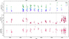 |
Fig. 1. Multi-wavelength light curve of 1ES 0229+200 presenting long-term (2008–2024) observations of the blazar. The panels present optical Swift-UVOT observation in U, B, V filters; X-ray (0.3–10 keV) flux; and corresponding power-law photon index. Two epochs of NuSTAR observations taken in 2013 and 2021 are marked with vertical lines and noted as nu13 and nu21, respectively. |
The temporal variability observed in the light curve can be quantified using the fractional variability amplitude, as defined by Vaughan et al. (2003) and Poutanen et al. (2008) as
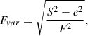 (4)
(4)
where S2 is the variance, e2 is the mean square error, and F is the mean flux. The uncertainties of Fvar are calculated following the formula by Poutanen et al. (2008):
 (5)
(5)
with the error in the normalised excess variance σ given as (Vaughan et al. 2003)
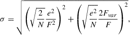 (6)
(6)
where N is the number of data points in the light curve.
Consistent with previous findings for 1ES 0229+200, the long-term variability in the X-ray band (0.3–10 keV) is more pronounced than in the optical bands. The X-ray light curve exhibits considerable variability, with long-term flux variations of a factor of three, while the optical V, B, and U bands show only marginal variability. This corresponds to fractional variability amplitudes (Fvar) of 31%±1% for the X-ray band and around (5 − 12)% ± 2% for the opticalfrequencies.
Due to the limited number of NuSTAR observations, it is not feasible to determine the fractional variability amplitude for these data. However, for each NuSTAR observation, the fluxes in the 3–10 keV and 3–40 keV energy bands were calculated and are summarised in Table 4. These flux measurements confirm a significantly lower X-ray flux level in the 2021 observations compared to the 2013 data. The lower X-ray-flux level is also notable for the Swift-XRT observations of the blazar taken for the same period. Furthermore, in the case of the 2021 NuSTAR observation of 1ES 0229+200notable flux variability between individual observations within both energy bands is evident, confirming daily variability also in the hardX rays.
Summary of X-ray fluxes.
3.2. Correlations
Simultaneous X-ray and optical observations of 1ES 0229+200 were performed with Swift-XRT and NuSTAR, respectively. Fig. 2 shows comparison of of the optical and X-ray fluxes. That includes a flux-flux comparison for the Swift/UVOT B and V filters; the optical B filter and Swift-XRT 0.3–10 keV flux; the colour-magnitude diagram for optical V and B filters; and a comparison of the X-ray 0.3–10 keV flux and corresponding photon index. For all cases, each point in a plot corresponds to a single Swift observation, and only simultaneous observations (with the same ObsID) are considered here.
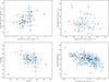 |
Fig. 2. Correlation plots for 1ES 0229+200. The following figures present flux-flux comparison of Swift/UVOT V and B filter; flux-flux comparison of Swift/UVOT V flux and Swift-XRT flux measured in the energy range of 0.3–10 keV; colour-magnitude diagram for V magnitude and B − V colour; flux-index comparison for Swift-XRT observations. |
The main results of the correlation analysis are listed below.
-
(i)
The optical Swift/UVOT B and V fluxes show a slight correlation, with a Pearson correlation coefficient of 0.5 ± 0.11. The relation is weak, which can be attributed to several factors, including the lack of correction for host-galaxy contamination and large uncertainties due to the short exposures used in the comparison.
-
(ii)
Simultaneous X-ray and optical observations do not reveal any apparent correlation. The Pearson correlation coefficient for this relation is −0.13 ± 0.09, indicating an absence of any significant trend. The lack of correlation between optical and X-ray fluxes probably results from the low variability in the optical band compared to the significant flux changes observed in X-rays (see e.g. Fig. 1).
-
(iii)
The colour–magnitude diagram shows a clear correlation, with a coefficient of 0.5 ± 0.1. Although still a weak trend, it can be explained by the same effects noted in (i). This bluer-when-brighter behaviour has previously been reported for 1ES 0229+200 based on long-term optical monitoring (e.g. Wierzcholska et al. 2015).
-
(iv)
A negative correlation is observed between the X-ray flux and photon index, with a Pearson coefficient of 0.52 ± 0.04, indicating a harder-when-brighter trend in the 0.3–10 keV X-ray band.
3.3. Spectral properties
In the spectral analysis, we focused on the 2021 NuSTAR data (ObsID 10702609002-10702609006) and the corresponding simultaneous Swift-XRT observations. The details of the simultaneous Swift-XRT data used are listed in Table 1. All NuSTAR spectra were fitted using three different models: a single power-law, log-parabola, and a broken power-law, each including the Galactic column density as provided by Willingale et al. (2013). Table 2 presents the resulting fitting parameters for all tested models for the NuSTAR observations, while Table 3 presents all spectral parameters for the power-law fits to the X-ray data. The errors for all parameters are quoted at the 1-σ confidence level. For comparison, Table 2 also includes the spectral parameters of the power-law and log-parabola fits to the 2013 NuSTAR data. Since there is no clear preference for a curved spectral shape in this case, the parameters of the broken power-law model are not included in the table.
Figure 3 shows the NuSTAR spectra for different epochs of NuSTAR observations of the blazar, from both 2013 and 2021. To provide a wider range of X-ray spectral data for 1ES 0229+200, simultaneous Swift-XRT observations are also included for all NuSTAR observations. In the case of the X-ray spectral presented in Fig. 3, the Swift-XRT and NuSTAR data points are the results of the separate fitting of the observations taken with these two instruments. For all three observations, the χ2 values and spectral shapes of the 2021 NuSTAR spectra, visible in Fig. 3, indicate a hard X-ray excess above 25 keV. Such a spectral feature was not detected in the NuSTAR observations of the blazar performed in 2013.
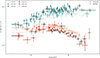 |
Fig. 3. Spectral energy distributions presenting NuSTAR and Swift-XRT observations for six epochs (3 in 2013 and 2021). Swift-XRT observations are corrected for the influence of the hydrogen Galactic column density with NH provided by Willingale et al. (2013). The last two digits of the label denote the ObsIDs of the NuSTAR observations. The Swift-XRT and NuSTAR observations are distinguished by filled and hollow markers, respectively. The full ObsIDs are listed in Table 1. In the case of 2013 NuSTAR data, spectral points are adopted from Wierzcholska & Wagner (2020). |
To compare the goodness of fit among the three tested models, we employed the F-test (e.g. Bevington & Robinson 2003). This allowed us to assess whether adding an extra parameter to a more complex model—accounting for either curvature or a spectral break—provides a statistically significant improvement over the simpler single-power-law model. The test was applied to all three NuSTAR observations obtained in 2021. The hard X-ray excess is most clearly visible in the observation labelled nu21_04, and this is confirmed by the F-test results, which indicate that the inclusion of the additional parameter in the more complex model yields a highly significant improvement in the fit, at a confidence level exceeding 4σ (p ≪ 0.001). For observations nu21_02 and nu21_06, the improvement is still present but less pronounced, reaching only the 1–2σ level(p ≈ 0.1).
4. Discussion
The analysis of NuSTAR observations of 1ES 0229+200 from August 2021 revealed that the source was in a low-flux X-ray state, evident in energies up to ∼40 keV. This period, marked by the second NuSTAR campaign targeting 1ES 0229+200, is clearly characterised by a low-X-ray state, as seen in the long-term 0.3–10 keV light curve of the blazar.
These NuSTAR observations also revealed a concave spectral shape with a notable upturn of around 25 keV. Such an upturn in the X-ray range had not been reported before, neither in previous NuSTAR observations nor in Swift-BAT data. Furthermore, spectral modelling by Kaufmann et al. (2011) suggests that the X-ray emission of 1ES 0229+200 extends up to 100 keV without any cut-off or spectral upturn.
Here, we report a distinct concave spectral shape observed in all three observations from August 2021, with the upturn located at 25–26 keV. Despite temporal variability in these observations, with changes in the 3–10 keV flux of approximately 20%, the position of the spectral upturn remains consistent within the parameter uncertainties.
To explore the origin of the X-ray excess above 25 keV, several scenarios can be considered. One possible explanation for the concave X-ray spectrum is the presence of a spectral crossing point in this energy range, where the synchrotron and inverse Compton components converge. Interestingly, similar spectral upturns, linked to the presence of synchrotron and inverse Compton components, have been detected in the 0.3–10 keV X-ray band for several IBL-type blazars (see e.g. Wierzcholska & Wagner 2016). The authors also suggested that for some IBL-type blazars, the spectral upturn may be located in the X-ray domain, but above 10 keV.
For HBL-type sources, a concave X-ray spectrum has been observed in only a few cases, such as PKS 2155-304 and Mrk 421 (Zhang 2008 and Kataoka & Stawarz 2016, respectively). In the latter case, the spectral upturn was detected during the NuSTAR observation of the source’s low state, but was absent in high-state observations of Mrk 421.
Alternatively, the three-bump SED of blazars, as indicated by the NuSTAR spectrum of 1ES 0229+200, may be explained by a photohadronic origin. For HBL-type blazars, the energy range of 40 keV to 40 MeV is where a third SED bump might be visible. It is well established that both electrons and protons can be accelerated to relativistic energies and may contribute to the broadband emission observed (see e.g. Biermann & Strittmatter 1987; Sironi et al. 2013). In the leptohadronic scenario, the low-energy component of the SED is explained by synchrotron emission from relativistic electrons, whereas the high-energy component involves interactions of relativistic protons in the jets. Petropoulou & Mastichiadis (2015) demonstrated that Bethe-Heitler pair production and photopion production playsignificant roles in this process. The authors showed that when relativistic protons interact with synchrotron photons in blazars, leading to gamma-ray production through photopion processes, the SED is affected by two key features: PeV neutrino emission and a third SED bump located in the keV–MeV energy range. A natural implication of this scenario and the leptohadronic origin of blazar emission is the potential for high-energy neutrino emission from blazars exhibiting athree-bump SED.
Having observational constraints, the best way to distinguish between different possible scenarios describing physical processes responsible for a broadband emission is a modelling. However, in the case of 1ES 0229+200, due to the weakness of high-energy γ-ray emission, it is not possible to constrain the Fermi-LAT spectrum using a few days or even a few weeks of data. Thus, a discussion of this energy regime in terms of the low state of 1ES 0229+200 is not possible (see e.g. Cologna et al. 2015).
Considering the discussion provided by Wierzcholska & Wagner (2020) on the host galaxy, spectral curvature, absorption, and ultraviolet excess features in the broadband SED of 1ES 0229+200, we argue that the feature detected in the low-state spectrum in this work is more likely attributed to photohadronic processes. That is also supported by the consideration of signatures of the Bethe-Heitler emission in the blazars’ broadband SEDs provided by Petropoulou & Mastichiadis (2015). Assuming this scenario, 1ES 0229+200 should also be considered a potential source of high-energy neutrino emission.
Furthermore, it should be noted that in previous X-ray observations of 1ES 0229+200 conducted by NuSTAR and Swift-BAT, the upturn was not observed. This can be explained by the higher X-ray state of the source compared to the August 2021 observations discussed in this work.
Errors for the Pearson correlation coefficients are calculated as described by Wierzcholska (2015).
Acknowledgments
The project is co-financed by the Polish National Agency for Academic Exchange. The authors gratefully acknowledge the Polish high-performance computing infrastructure PLGrid (HPC Centre: ACK Cyfronet AGH) for providing computer facilities and support within computational grant no. PLG/2024/017925. This research has made use of the NuSTAR Data Analysis Software (NuSTARDAS) jointly developed by the ASI Space Science Data Center (SSDC, Italy) and the California Institute of Technology (Caltech, USA).
References
- Abdo, A. A., Ackermann, M., Agudo, I., et al. 2010, ApJ, 716, 30 [NASA ADS] [CrossRef] [Google Scholar]
- Aharonian, F., Akhperjanian, A. G., Barres de Almeida, U., et al. 2007, A&A, 475, L9 [CrossRef] [EDP Sciences] [Google Scholar]
- Aliu, E., Archambault, S., Arlen, T., et al. 2014, ApJ, 782, 13 [NASA ADS] [CrossRef] [Google Scholar]
- Arnaud, K. A. 1996, ASP Conf. Ser., 101, 17 [Google Scholar]
- Begelman, M. C., Blandford, R. D., & Rees, M. J. 1984, Rev. Mod. Phys., 56, 255 [Google Scholar]
- Bevington, P. R., & Robinson, D. K. 2003, Data Reduction and Error Analysis for the Physical Sciences (McGraw-Hill) [Google Scholar]
- Bhatta, G., Mohorian, M., & Bilinsky, I. 2018, A&A, 619, A93 [NASA ADS] [CrossRef] [EDP Sciences] [Google Scholar]
- Biermann, P. L., & Strittmatter, P. A. 1987, ApJ, 322, 643 [Google Scholar]
- Böttcher, M., Reimer, A., Sweeney, K., & Prakash, A. 2013, ApJ, 768, 54 [Google Scholar]
- Cenko, B. 2023, GCN, 34633, 1 [Google Scholar]
- Cologna, G., Mohamed, M., Wagner, S., et al. 2015, Int. Cosm. Ray Conf., 34, 762 [Google Scholar]
- Ehlert, S. R., Liodakis, I., Middei, R., et al. 2023, ApJ, 959, 61 [NASA ADS] [CrossRef] [Google Scholar]
- Elvis, M., Plummer, D., Schachter, J., & Fabbiano, G. 1992, ApJS, 80, 257 [CrossRef] [Google Scholar]
- Furniss, A., Noda, K., Boggs, S., et al. 2015, ApJ, 812, 65 [NASA ADS] [CrossRef] [Google Scholar]
- Giommi, P., Ansari, S. G., & Micol, A. 1995, A&AS, 109, 267 [NASA ADS] [Google Scholar]
- Giommi, P., Blustin, A. J., Capalbi, M., et al. 2006, A&A, 456, 911 [NASA ADS] [CrossRef] [EDP Sciences] [Google Scholar]
- Harrison, F. A., Craig, W. W., Christensen, F. E., et al. 2013, ApJ, 770, 103 [Google Scholar]
- Kataoka, J., & Stawarz, Ł. 2016, ApJ, 827, 55 [NASA ADS] [CrossRef] [Google Scholar]
- Kaufmann, S., Wagner, S. J., Tibolla, O., & Hauser, M. 2011, A&A, 534, A130 [NASA ADS] [CrossRef] [EDP Sciences] [Google Scholar]
- Mannheim, K. 1993, A&A, 269, 67 [NASA ADS] [Google Scholar]
- Marscher, A. P. 1980, ApJ, 235, 386 [NASA ADS] [CrossRef] [Google Scholar]
- Murase, K., Guetta, D., & Ahlers, M. 2016, Phys. Rev. Lett., 116, 071101 [NASA ADS] [CrossRef] [Google Scholar]
- Oikonomou, F., Petropoulou, M., Murase, K., et al. 2021, JCAP, 2021, 082 [CrossRef] [Google Scholar]
- Padovani, P., & Giommi, P. 1995, MNRAS, 277, 1477 [NASA ADS] [CrossRef] [Google Scholar]
- Pandey, A., Gupta, A. C., & Wiita, P. J. 2017, ApJ, 841, 123 [NASA ADS] [CrossRef] [Google Scholar]
- Petropoulou, M., & Mastichiadis, A. 2015, MNRAS, 447, 36 [NASA ADS] [CrossRef] [Google Scholar]
- Petropoulou, M., Dimitrakoudis, S., Padovani, P., Mastichiadis, A., & Resconi, E. 2015, MNRAS, 448, 2412 [Google Scholar]
- Petropoulou, M., Murase, K., Santander, M., et al. 2020, ApJ, 891, 115 [Google Scholar]
- Poole, T. S., Breeveld, A. A., Page, M. J., et al. 2008, MNRAS, 383, 627 [Google Scholar]
- Poutanen, J., Zdziarski, A. A., & Ibragimov, A. 2008, MNRAS, 389, 1427 [Google Scholar]
- Rector, T. A., Gabuzda, D. C., & Stocke, J. T. 2003, AJ, 125, 1060 [NASA ADS] [CrossRef] [Google Scholar]
- Reimer, A., Böttcher, M., & Buson, S. 2019, ApJ, 881, 46 [Google Scholar]
- Sahakyan, N. 2021, ApJ, 910, 32 [Google Scholar]
- Schlafly, E. F., & Finkbeiner, D. P. 2011, ApJ, 737, 103 [Google Scholar]
- Sironi, L., Spitkovsky, A., & Arons, J. 2013, ApJ, 771, 54 [Google Scholar]
- Tavecchio, F., & Ghisellini, G. 2010, MNRAS, 406, L70 [CrossRef] [Google Scholar]
- Urry, C. M., Scarpa, R., O’Dowd, M., et al. 2000, ApJ, 532, 816 [NASA ADS] [CrossRef] [Google Scholar]
- Vaughan, S., Edelson, R., Warwick, R. S., & Uttley, P. 2003, MNRAS, 345, 1271 [Google Scholar]
- Wagner, S. J., & Witzel, A. 1995, ARA&A, 33, 163 [NASA ADS] [CrossRef] [Google Scholar]
- Wierzcholska, A. 2015, A&A, 580, A104 [NASA ADS] [CrossRef] [EDP Sciences] [Google Scholar]
- Wierzcholska, A., & Wagner, S. J. 2016, MNRAS, 458, 56 [NASA ADS] [CrossRef] [Google Scholar]
- Wierzcholska, A., & Wagner, S. J. 2020, MNRAS, 496, 1295 [NASA ADS] [CrossRef] [Google Scholar]
- Wierzcholska, A., Ostrowski, M., Stawarz, Ł., Wagner, S., & Hauser, M. 2015, A&A, 573, A69 [NASA ADS] [CrossRef] [EDP Sciences] [Google Scholar]
- Willingale, R., Starling, R. L. C., Beardmore, A. P., Tanvir, N. R., & O’Brien, P. T. 2013, MNRAS, 431, 394 [Google Scholar]
- Woo, J.-H., Urry, C. M., van der Marel, R. P., Lira, P., & Maza, J. 2005, ApJ, 631, 762 [Google Scholar]
- Zhang, Y. H. 2008, ApJ, 682, 789 [NASA ADS] [CrossRef] [Google Scholar]
- Zhang, H., Fang, K., Li, H., et al. 2019, ApJ, 876, 109 [NASA ADS] [CrossRef] [Google Scholar]
All Tables
All Figures
|
Fig. 1. Multi-wavelength light curve of 1ES 0229+200 presenting long-term (2008–2024) observations of the blazar. The panels present optical Swift-UVOT observation in U, B, V filters; X-ray (0.3–10 keV) flux; and corresponding power-law photon index. Two epochs of NuSTAR observations taken in 2013 and 2021 are marked with vertical lines and noted as nu13 and nu21, respectively. |
| In the text | |
|
Fig. 2. Correlation plots for 1ES 0229+200. The following figures present flux-flux comparison of Swift/UVOT V and B filter; flux-flux comparison of Swift/UVOT V flux and Swift-XRT flux measured in the energy range of 0.3–10 keV; colour-magnitude diagram for V magnitude and B − V colour; flux-index comparison for Swift-XRT observations. |
| In the text | |
|
Fig. 3. Spectral energy distributions presenting NuSTAR and Swift-XRT observations for six epochs (3 in 2013 and 2021). Swift-XRT observations are corrected for the influence of the hydrogen Galactic column density with NH provided by Willingale et al. (2013). The last two digits of the label denote the ObsIDs of the NuSTAR observations. The Swift-XRT and NuSTAR observations are distinguished by filled and hollow markers, respectively. The full ObsIDs are listed in Table 1. In the case of 2013 NuSTAR data, spectral points are adopted from Wierzcholska & Wagner (2020). |
| In the text | |
Current usage metrics show cumulative count of Article Views (full-text article views including HTML views, PDF and ePub downloads, according to the available data) and Abstracts Views on Vision4Press platform.
Data correspond to usage on the plateform after 2015. The current usage metrics is available 48-96 hours after online publication and is updated daily on week days.
Initial download of the metrics may take a while.