| Issue |
A&A
Volume 703, November 2025
|
|
|---|---|---|
| Article Number | A181 | |
| Number of page(s) | 9 | |
| Section | Stellar structure and evolution | |
| DOI | https://doi.org/10.1051/0004-6361/202555328 | |
| Published online | 20 November 2025 | |
Variability of the DG Tau forbidden emission line low velocity component⋆
1
Department of Physics, Maynooth University, Maynooth, Co.Kildare, Ireland
2
European Southern Observatory, Alonso de Córdova 3107, Vitacura, Casilla 19001, Santiago de Chile, Chile
3
Institute of Astronomy and Astrophysics, Academia Sinica, 11F of Astronomy-Mathematics Building, No.1, Sec. 4, Roosevelt Rd, Taipei 10617, Taiwan, R.O.C
4
Max-Planck-Institut für Extraterrestrische Physik, Gießenbachstraße 1, 85748 Garching bei München, Germany
5
Department of Physics, Texas State University, 749 N Comanche Street, San Marcos, TX 78666, USA
⋆⋆ Corresponding author: This email address is being protected from spambots. You need JavaScript enabled to view it.
Received:
28
April
2025
Accepted:
22
September
2025
Abstract
Context. Optical forbidden emission lines (FELs) come from transitions with long radiative decay times (≈100 s) that require low density environments where collisions between atoms are rare. They are produced in the low-density gas found in the outflows (jets and winds) driven by low-mass young stellar objects (YSOs). Moreover, they frequently reveal distinct velocity components within the outflow, including a so-called low velocity component (LVC). A question pertinent to the removal of excess angular momentum in YSOs is whether the LVC traces a magnetohydrodynamic (MHD) wind or a photoevaporative wind. Here, we study the jet and LVC of the classical T Tauri Star DG Tau. The velocity of the DG Tau jet has been decreasing since 2006, making it a particularly interesting source for this work.
Aims. The aim is to investigate the connection between the high-velocity jet and the LVC in DG Tau and to better understand the origin of the LVC by examining spectral and spatial changes over time.
Methods. Kinematic fitting and spectro-astrometry were applied to three epochs of high spectral resolution data spanning ≈18 years to conduct a detailed study of the changes in the LVC over time.
Results. A decrease in velocity of ≈100 kms−1 from 2003 to 2021 is in agreement with the known slowing of the DG Tau jet. The kinematic fitting of the [O I]λ6300, [O I] λ5577, and [S II] λ6731 lines over the three epochs of data reveal the complex nature of the optical FELs. In agreement with a recent study of the DG Tau optical FELs, up to six blueshifted components in the FEL line profiles alongside a redshifted wing are identified. The three observed LVC sub-components (LVC-high, LVC-medium, and LVC-low) are consistent with entrained jet material, a disk wind, and a dense upper disk atmosphere, respectively. Despite the strong variability of the jet components over the three epochs, the LVC is found to be far more stable, and only the relative brightness of the three LVC sub-components is seen to change. A constraint of ≥2 au is placed on the minimum de-projected height of the LVC-M in [O I] λ5577 where there is no contribution from the jet.
Conclusions. The results support a disk wind origin for the LVC-M sub-component but cannot distinguish between a photoevaporative or MHD wind origin. The minimum [O I] λ5577 LVC-M height of ≥2 au indicates that this wind is launched inside the gravitational potential well of DG Tau and favours an MHD wind origin for the LVC-M. The fact that the peak velocity of the LVC-M does not change significantly requires further investigation in the context of a common origin for jets and MHD disk winds. Future studies will benefit from higher spectral resolution data to reduce blending between the outflow components and higher cadence sampling in time to explore a time lag between changes in the jet and the LVC.
Key words: stars: formation / stars: jets / stars: low-mass / stars: variables: T Tauri / Herbig Ae/Be / stars: winds / outflows
Based on observations made with ESO Telescopes at the La Silla Paranal Observatory under programme IDs 384.C-0821(B) and 108.22M8.001 and on data collected by High Dispersion Spectrograph (HDS) at Subaru Telescope which is operated by the National Astronomical Observatory of Japan. We are honored and grateful for the opportunity to observe the Universe from Maunakea, which has cultural, historical, and natural significance in Hawaii.
© The Authors 2025
 Open Access article, published by EDP Sciences, under the terms of the Creative Commons Attribution License (https://creativecommons.org/licenses/by/4.0), which permits unrestricted use, distribution, and reproduction in any medium, provided the original work is properly cited.
This article is published in open access under the Subscribe to Open model. This email address is being protected from spambots. You need JavaScript enabled to view it. to support open access publication.
1. Introduction
Classical T Tauri stars (CTTSs) are class II low mass young stellar objects (YSOs) and the precursors of protoplanetary systems. They are active accretors and drive jets and winds (Ray et al. 2007). As a result, their spectra show an abundance of emission lines tracing accretion and outflow activity (Whelan et al. 2014). From early in the study of CTTSs, their FEL profiles were known to be multi-component (Hartigan et al. 1995), with a frequently spatially extended high-velocity component (HVC, |v| > 100 kms−1) tracing the collimated jet (Hirth et al. 1997), and a spatially compact low velocity component (LVC, |v| < 40 kms−1) tracing a wind (Kwan & Tademaru 1988). This wind could be a magnetohydrodynamic (MHD) wind and therefore connected to the jet (Pascucci et al. 2025; Birney et al. 2024), or a photoevaporative wind and thus thermally driven (Rab et al. 2023). Recently, there has been renewed interest in the forbidden emission line (FEL) LVC as a means of investigating whether the MHD winds solve the angular momentum transport problem in YSOs (Pascucci et al. 2025). Recent simulations (Bai 2016) that include non-ideal MHD effects have shown that low-velocity winds in the inner disk are critical in providing the spin-down torques needed to remove excess angular momentum, hence enabling stellar mass accretion. Finding an observational tracer of these winds and testing the findings of these simulations is critical in understanding angular momentum transport in YSOs. The FEL LVC is a promising potential tracer of these low-velocity winds and as such, may be important in the removal of excess angular momentum in these young stellar systems. However, the compact nature of the LVC presents an observational challenge to understanding its origin. Two methods have been used to address the compact nature of the LVC and study it. These are the kinematic fitting of the line profiles through Gaussian decomposition (Banzatti et al. 2019) and spectro-astrometry, which recovers spatial information from compact emission line regions (Whelan & Garcia 2008).
Previous literature regarding the LVC (e.g. Simon et al. 2016; McGinnis et al. 2018; Fang et al. 2018; Nisini et al. 2024) used kinematic fitting to show that the LVC can be further divided into sub-components. These studies observed both a broad and narrow LVC sub-component in FEL profiles. These broad and narrow sub-components are separated on the basis of their measured full width at half maximum (FWHM). The broad sub-component, referred to as the LVC-BC, has an FWHM ≥ 40 kms−1, whereas the narrow sub-component, referred to as the LVC-NC, has an FWHM ≤ 40 kms−1. Fang et al. (2018) found a statistical correlation between the [O I] λ6300 line luminosity of the HVC and LVC to the stellar accretion luminosity in a sample of 48 stars. They find that the LVC-BC is more tightly correlated with the stellar accretion luminosity than the LVC-NC. They also find that the ratio of [O I] λ5577 to [O I] λ6300 differs between the LVC-BC and the HVC. These findings combined corroborate the idea that the LVC-BC traces a hot and dense region of gas close to the base on an MHD disk wind.
Banzatti et al. (2019) expanded the work of Simon et al. (2016) and Fang et al. (2018) to a sample of 65 stars. They find correlations between the kinematics of the LVC (centroid velocity and FWHM) to the equivalent width of the HVC and the stellar accretion luminosity. This work reinforces the idea that the LVC-BC traces the dense and hot base of an MHD disk wind. The origin of the LVC-NC remains a matter of debate. Previous literature indicates that the LVC-NC may be part of an MHD wind (Fang et al. 2018; Banzatti et al. 2019) or that the LVC-NC sub-component can be produced by photoevaporative winds (Rab et al. 2023). A key deficiency of these kinematic fitting studies of many young stars is the lack of spatial information. The poor constraint on the vertical extent of the emission traced by these LVC sub-components above the disk mid-plane limits the accuracy of the derived mass outflow rates. The LVC is compact, so measuring the height of the LVC emission above disk mid-plane presents a challenge. The technique of spectro-astrometry can be used to address this and provide critical constraints on the vertical extent of the emission traced by these LVC sub-components.
For example, Whelan et al. (2021) applied spectro-astrometry to optical spectra from the star RU Lupi in order to study its FEL LVC. Spectro-astrometry involves the fitting of a Gaussian to spatial profiles extracted perpendicular to the dispersion axis of a 2D spectrum. The peak position of each fit to a spatial profile is called a spatial centroid. These spatial centroids can be plotted as a function of velocity, and the result is referred to as a position spectrum. Position spectra measure the centroid offset of the brightest extended emission traced by an emission line region relative to the position of the star. The work of Whelan et al. (2021) provided better constraints on the vertical extent of the emission above the disk mid-plane compared to the previous kinematic fitting studies. Their results show a negative velocity gradient in the region of the position spectrum related to the LVC-NC sub-component. A negative velocity gradient in a position spectrum refers to an increase in the recorded position centroid offset with decreasing velocity. Physically it means a decrease in the velocity of the emission traced by the spectro-astrometry in the forbidden emission line region as the height above the disk mid-plane increases. Modelling has shown that this negative gradient is indicative of a disk wind (Pontoppidan et al. 2011). The spectro-astrometry of Whelan et al. (2021) traced the extent of the LVC-NC to 2 au. This is within the gravitational potential well of RU Lupi and provides evidence that this LVC-NC sub-component may be tracing an MHD disk wind.
Conversely, a positive velocity gradient in the position spectrum refers to an increase in the recorded position centroid offset with increasing velocity. Physically it means an increase in the velocity of the emission traced by the spectro-astrometry in the forbidden emission line region as height above the disk mid-plane increases. This positive gradient is a feature of jets (Hirth et al. 1997), and close to the source, it is indicative of the jet launching process. At greater distances from the source, this positive velocity gradient could be caused by entrainment or material ejected at higher velocities accelerating slower jet material (Davis et al. 2001; Whelan et al. 2004). Eventually, for the high-velocity region, the spectro-astrometric signal changes, so that a decrease in offset is recorded with velocity, which often coincides with knots in the jet (see Figs. 3 and 5 of Whelan et al. 2004). These positive velocity gradients have also been observed in previous studies that have used spectro-astrometry (Whelan et al. 2024).
Many CTTS jets show kinematic variability, which could be connected to variable accretion (Pyo et al. 2024; Takami et al. 2023). If the LVC traces a MHD wind, then it is reasonable to expect that it will vary with a variable HVC. The disk wind model for jet launching purports that the jet is the inner part of the larger MHD disk wind, which becomes collimated by magnetic fields (Ferreira et al. 2006). Therefore, additional information on the origin of the LVC could be gleaned by studying variability. Variability of the LVC has been previously noted in the literature (Simon et al. 2016; Nisini et al. 2024). However, no dedicated study of the variability of the LVC has been conducted to date. This article is the first dedicated study of variation in the LVC over time.
We note here that Takami et al. (2023) report a decrease by a factor of two in the tangential velocity of the DG Tau blueshifted jet over a twenty year period, pointing to a remarkable change in the velocity at which DG Tau ejects material. This makes DG Tau a particularly interesting object in which to study the LVC. The goal of the work presented here is to determine if spectral and spatial changes in the DG Tau HVC are accompanied by corresponding changes in the LVC.
This article expands on the previous literature and presents a dedicated study of the variability in the blueshifted LVC sub-components of DG Tau for three optical FELs. We used kinematic fitting and applied spectro-astrometry to three epochs of high resolution spectra covering the FELs [O I] λ5577, [O I] λ6300, and [S II] λ6731. These lines are selected because they have very different critical densities, decreasing from ∼108 cm−3 for [O I] λ5577 to ∼104 cm−3 for [S II]λ6731; hence, they trace different parts of the outflow system (Giannini et al. 2019).
In a recent work, Chou et al. (2025) used kinematic fitting and spectro-astrometry to isolate six different blueshifted emission components in the FELs of DG Tau. They find two HVCs (HVC1 and HVC2), a medium velocity component (MVC) and three LVCs, (LVC-High, LVC-Medium and LVC-Low) for high, medium, and low velocities within the LVC. Hereafter, we refer to these LVC sub-components as the LVC-H, LVC-M, and LVC-L respectively. They argue that the HVC1 and HVC2 trace the extended jet and a stationary shock at the jet base, respectively. Chou et al. (2025) also used line ratios and modelling to conclude that the LVC-H, LVC-M, and LVC-L are associated with an interaction region between the jet and disk wind, a disk wind and the upper disk atmosphere, respectively. Their data is the first epoch of data used for our time variability study. Thus, for consistency we refer to the velocity components observed in this article using the nomenclature of Chou et al. (2025). The rest of the article is organised as follows: Section 2 outlines the observations undertaken, along with the steps performed for data reduction and analysis. In Sect. 3 we present the position-velocity (PV) diagrams and the results of our kinematic and spectro-astrometric analysis. Lastly, in Sect. 4 we discuss our findings and draw our conclusions from these results.
2. Observations, data reduction, and analysis
DG Tau (Table 1) was observed in 2003 with SUBARU/HDS (Chou et al. 2025) and in 2010 and 2021 with the Ultraviolet and Visual Echelle Spectrograph (UVES; Dekker et al. 2000) on the Very Large Telescope (Table 2). The instrument slits were parallel to the known jet position angle (PA). The details regarding the reduction of the data from 2003 is presented in Chou et al. (2025). The UVES data were reduced using the UVES pipeline (version 6.1.6; Freudling et al. 2013) to produce 2D spectra. The PV diagrams were constructed (Fig. 1) from the full spatial range of these 2D spectra after continuum subtraction.
Properties of DG Tau.
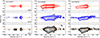 |
Fig. 1. Position-velocity diagrams of the [O I] λ5577 (left), [O I] λ6300 (middle), and [S II] λ6731 (right) FELs in 2003, 2010, and 2021 from DG Tau. Contours start at 3σ (2003) and 7σ (2010, 2021) above the background rms noise and increase by factors of |


Observation log.
The continuum subtraction was preformed on each 2D spectrum of the [O I] λ5577, [O I] λ6300, and [S II] λ6731 lines following this procedure. A Python script first masked the regions that contain emission or absorption features along each dispersion axis in the spectrum. Following this, a polynomial was fit to the unmasked regions to obtain an estimate of the continuum along each dispersion axis. The estimated continuum was then subtracted from the 2D spectrum in a line-by-line fashion to remove the stellar contribution from the spectrum.
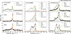 |
Fig. 2. Kinematic fitting comparison of the [O I] λ5577, [O I] λ6300, and [S II] λ6731 line profiles via Gaussian decomposition in 2003, 2010, and 2021. The line profiles are shown in the stellocentric frame and are normalised to the continuum level. These profiles are extracted over the full spatial range of the PV diagrams shown in Fig.1. |
1D spectral line profiles were then extracted from these 2D continuum subtracted spectra. The region in which the line profiles were extracted covers the whole spatial range of the 2D data. The line profiles were then corrected for telluric and photospheric absorption features using the ESO MOLECFIT pipeline (Smette et al. 2015; Kausch et al. 2015) and the photospheric correction method outlined in Hartigan et al. (1989). The kinematic fitting of the 1D spectra was then carried out following the procedure of Chou et al. (2025). This method involves fitting a composite model of independent Gaussian components to reproduce the line profile. The number of required Gaussian components for the model was determined via a reduced chi-square minimisation. Additional Gaussian components were added to the model only when the reduced chi-square improved by at least a factor of 20% compared to the composite model with one fewer Gaussian components.
All velocities quoted in this work are in the stellocentric frame. In order to convert the line profiles from the topocentric frame into the stellocentric frame, two velocity corrections were applied to the line profiles. The stellar radial velocity correction was calculated following Pascucci et al. (2015). The heliocentric velocity correction was calculated using the radial_velocity_correction function available in Astropy (Astropy Collaboration 2013, 2018, 2022). The rvcorrect method available in the Image Reduction and Analysis Facility (IRAF) was also used to confirm the accuracy of the heliocentric velocity correction calculated using Astropy. The uncertainties on the centroid velocity (Vc) and the FWHM values obtained from the kinematic fitting were calculated following the method of Nisini et al. (2024). These uncertainties were significantly less than the uncertainty calculated for the radial velocity of the source (0.5 kms−1). Therefore, this latter value was taken as the uncertainty on the kinematic fitting values.
Spectro-astrometry was applied to the 2D spectra before and after continuum subtraction as outlined in Whelan et al. (2021). This was done to prevent the stellar brightness contribution from contaminating the offset measured in the position spectrum for the brightest extended emission. The centroids measured for the extended emission before continuum subtraction were pulled back to the stellar position due to the stellar contribution to the 2D spectrum. The stellar continuum was subtracted, as outlined in the previous paragraphs, and the spatial centroids were re-measured less the continuum. The 1σ uncertainty on the recovered position of the extended emission is given by Eq. (1). This depends on the signal to noise ratio (S/N) of the spatial profiles (Whelan & Garcia 2008). In Eq. (1), Np is the number of detected photons, and the FWHM of the spatial profile is an approximate measure of the seeing. For the HDS observations, anti-parallel slit PAs were used to correct for spatial artefacts. For the UVES data, anti-parallel slit PAs were not available, and spatial artefacts were ruled out by examining the spectro-astrometric position spectra in lines where no centroid offset was expected (Whelan et al. 2009).
 (1)
(1)
3. Results
Due to the relative faintness of the redshifted outflow only the blueshifted outflow was studied. Using the PV diagrams and kinematic fitting discussed in Sect. 2 (Table 3; Figs. 1 and 2), all the kinematic components first identified by Chou et al. (2025) were found but not in all lines or all years. Once identified they were investigated further using spectro-astrometry. The differences between the emission line regions can be explained in terms of their different critical densities and the decreasing electron density of the outflow with distance from the star. [O I] λ5577 traces the densest and, therefore, the most compact components. [O I] λ6300 is the most complex with contributions from all the identified kinematic components. [S II] λ6731 traces the most extended emission. In Figs. 3 and 4, for example, the [S II] λ6731 emission is extended up to twice the distance of the [O I] λ6300 emission. The HVC2 and LVC-L are not identified in the [S II] λ6731 line. Chou et al. (2025) argue that, this is because the critical density of [S II] λ6731 is too low. The effectiveness of the kinematic fitting for identifying the different velocity components is limited by the relative brightness of the components. It should be noted that a non-detection by the kinematic fitting does not mean that a particular component is not present in the outflow. For example, even though the LVC-L is not detected in the kinematic fitting of the [S II] λ6731 line, it does not mean that it is not present. Its contribution may be quenched due to critical density effects. Nonetheless, it may still contribute to the overall line profile, as described further in Sect. 3.2. The results for the the kinematic components associated with the jet by Chou et al. (2025), HVC1, HVC2, MVC, and LVC-H), as well as the LVC-L and LVC-M sub-components, are now presented separately.
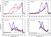 |
Fig. 3. Top row: Comparison of the line profiles of [O I] λ6300 and [S II] λ6731 for each epoch of data. The line profiles are normalised to max peak height to emphasise changes in the line shape over time. Bottom row: Position spectra for the [O I] λ6300 and [S II] λ6731 lines in 2003 (red), 2010 (blue), and 2021 (black). The analysis of the [O I] λ5577 line is not presented here, as it does not show an extended jet component due to its high critical density. |
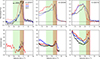 |
Fig. 4. Top row: Comparison of the line profiles in the LVC region of each FEL in each epoch of data. 2003 corresponds to the red line, 2010 corresponds to the blue line, and 2021 corresponds to the black line. These panels show a zoom-in on the line profiles shown in Fig. 3 from –90 to 50 kms−1. This is done to emphasise the change in line shape in the LVC region over time. The line profiles are normalised to max peak height. Bottom row: Position spectra of the LVC region for each FEL in each epoch of observation. 2003 corresponds to the red line, 2010 corresponds to the blue line, and 2021 corresponds to the black line. The 1σ uncertainties range from 1 to 5 au where 5 au is measured for the lowest S/N emission, i.e. [O I] λ5577 in 2021. |
Kinematic fitting of the blueshifted outflow components in kms−1.
3.1. Variability in the jet components
As the HVC1 is part of the extended jet it can be studied through PV diagrams and kinematic fitting. It is always present in [O I] λ6300 and [S II] λ6731, and its decrease in velocity by ∼100 kms−1 from 2003 to 2021 follows the known decrease in the jet velocity over this period (Takami et al. 2023; Pyo et al. 2024). In 2003 and 2010 in the extracted spectra shown in Fig. 2, it appears as a blue-wing and is not picked up by the kinematic fitting. To measure the 2003 and 2010 HVC1 velocity and FWHM for Table 3, a second spectrum extracted from the jet region was used. The extended jet does not have an excitation high enough to produce detectable emission in [O I]λ5577 with the exposure times and equipment used; hence, this component is not detected in the kinematic fitting or the PV plots of this emission line.
The HVC2 is detected in [O I] λ6300 in 2003 and 2010, in both the PV plots and the kinematic fitting, but not in 2021. In 2021 it is likely blended with the HVC1 and MVC. The [S II] λ6731 line does not trace this component and [O I] λ5577 traces the HVC2 in 2003 only. The decrease in the HVC2 velocity from 2003 to 2010 is in line with the decrease in the HVC1 velocity.
The MVC and LVC-H were not always detected, and in 2003 they were observed only together in [O I] λ6300 and [S II] λ6731. This is probably due to blending between the components as the velocity of the jet decreases. Chou et al. (2025) associate the LVC-H with a jet and wind interaction region. They do not discuss the origin of the MVC, but the decrease in the velocity of this component from 2003 to 2021 may suggest that it traces newly ejected lower-velocity knots that eventually become part of the extended jet.
Figure 3 presents the position spectra of the [O I] λ6300 and [S II] λ6731 line regions in the three epochs. The [O I] λ5577 line is not shown in this figure, as the extended jet is faint or absent in all epochs of data for this line. The strong variability in the centroids beyond ∼–75 kms−1 trace the changes in the jet, as the new knots are ejected with decreasing velocities. The region of the HVC1 initially shows a positive velocity gradient, as material is accelerated in the jet (Whelan et al. 2021). The peaks and troughs in the region of the position spectrum that covers the jet emission are typical of knotty jets, with the knots representing shocks in the outflow. For example, Fig. 5 of Whelan et al. (2004) and many of the figures presented in Hirth et al. (1997) show signatures in their position spectra consistent with knotty jets. The HVC2 is located at ∼30 au in [O I] λ6300 in 2010 in agreement with the Chou et al. (2025) analysis of the 2003 HDS spectra. The region of the MVC and LVC-H in both lines also has a positive velocity gradient, linking them to the jet, although in some cases the gradient is not steep.
3.2. Variability in the LVC
The LVC-M and LVC-L kinematic components are now discussed in terms of changes in the shape of the line profile, the peak velocities measured by the kinematic fitting, and the spatial properties of the emission regions as mapped with spectro-astrometry. These components are not spatially resolved in the PV diagrams of Fig. 1. The top row of Fig. 4 shows the LVC regions of each line profile with each epoch over-plotted. The lines are normalised to the line peaks so that changes in the LVC line profile shape are clear. As seen in Table 3, the peak velocities of these components do not vary greatly unlike the jet components. The range of LVC-M is marked in green in Fig. 4, and LVC-L is marked in red, with the overlap region appearing in light brown. This brown colour highlights the strong overlap between the two components, which impacts the kinematic fitting and spectro-astrometry. The line profile shape for all three lines changes substantially across the three epochs. This affects which components are detected by the kinematic fitting, as well as the measured peak velocities and peak centroids measured by spectro-astrometry.
For [O I] λ5577 in 2003, the line is at its widest and spans both the LVC-M and LVC-L components. The LVC-M is very prominent in this epoch, and therefore the kinematic fitting only detects an LVC-M. In 2010 and 2021, an LVC-L is detected by the kinematic fitting, but an LVC-M is not. What was previously identified as the LVC-M in 2003 has diminished to a blue-wing in later epochs. The peak velocities recorded for these components are consistent with the other emission lines.
The [O I] λ6300 LVC consists of a peak, an extended blue-wing, and a less substantial red-wing. In 2003 the kinematic fitting measures the line peak at –20 kms−1; this is identified as the LVC-M. A hump in the redshifted wing is measured at –9 kms−1 and identified as the LVC-L. The shape of the line profile changes substantially in 2010 and 2021. The LVC-M is associated with a blue-wing in 2010 and a hump in the blue-wing in 2021, rather than a clear peak as in 2003. The LVC-L, which appears as a hump in the red wing in 2003, is a clear line peak in 2010 and 2021. The peak velocity of the LVC-M increases from –20 kms−1 in 2003 to –27 kms−1 in 2010 and back to –22 kms−1 in 2021. We argue that this velocity variation for the LVC-M in [O I] λ6300 is due to blending with the MVC jet component, which is prominent in 2010 and the other changes to the line profiles described above. The peak velocity of the LVC-L does not vary by more than 2 kms−1.
The shape of the [S II] λ6731 LVC also changes between 2003 and 2021. The red wing seen in 2003 becomes a hump in 2010 and 2021. It could be that the LVC-L contributes to the line profile in 2010 and 2021, but this contribution is not picked up by the kinematic fitting. This interpretation of the changes observed in the [S II] λ6731 LVC aligns with the increase in the contribution of the LVC-L to both [O I] lines in those years. The strong and wide blueshifted emission peak seen in 2003 and 2010 reduces to a blue-wing in 2021. The peak velocity of the LVC-M increases from –30 kms−1 in 2003 to –40 kms−1 in 2010 and back to –20 kms−1 in 2021. Again, we argue that these changes to the peak velocity of the LVC-M is due to blending with the MVC jet component which is prominent in 2010 and the other changes to the line profiles described above.
The bottom row of Fig. 4 presents the position spectra of the LVC-M and LVC-L regions for all three FELs and in all three epochs after continuum subtraction. Strikingly, as highlighted above, while the shape of the LVC profiles changes greatly, the position spectra in this region remain very consistent across the nine measurements, considering both the velocities at which the peak centroids are measured and the velocity gradients. The biggest change in the velocity at which the maximum centroid is measured (∼–4 kms−1) occurs in the [O I] λ6300 emission region, where both the LVC-M and LVC-L have comparable contributions. In contrast, no such change in the velocity of the maximum offset is observed for the [S II] λ6731 measurements, in which the contribution of the LVC-L is minimised. For [O I] λ5577 the position spectrum is most similar to that seen in [O I] λ6300 and [S II]λ6731 in 2003 when the [O I] λ5577 emission was the least noisy.
The velocity gradients are also remarkably consistent. A positive gradient is seen for all lines at velocities more blueshifted than –25 kms−1 and it marks where we begin to see blending between the LVC and jet components begins. A negative velocity gradient, where offset increases with decreasing velocity, is indicative of a disk wind and is observed in all emission lines and in all epochs for the region covering 0 to –25 kms−1.
Where we do see variability in the position spectra is in the maximum and minimum values of the spatial centroids. If the LVC-L is tracing the upper disk atmosphere, it would be more compact than the extended disk wind traced by the LVC-M. As the components are blended, the measured centroids are a combination of the position of both components. Where contributions from the LVC-M and LVC-L to the overall line profile are comparable, as in [O I]λ6300, there is not much change in the maximum centroid between the years. In [S II] λ6731 the peak centroid decreases from ∼55 au in 2003 to ∼35 au in 2010 and 2021. This provides further evidence that the change in the blue-wing of the [S II] λ6731 emission in those years is due to an increased contribution from the LVC-L. The peak centroid is less in 2010 and 2021, as it includes a stronger contribution from the more compact LVC-L.
Also, we note that the spatial centroids of the [O I] λ5577 LVC-M reach a minimum value of 2 au at –25 kms−1 in 2003, while in [O I] λ6300 they are ∼ 15 au in all years and vary between 20 au and 32 au in [S II] λ6731. This provides evidence that the jet components combine with the LVC-M to increase the measured offset of the more compact LVC-M emission, similarly to how the LVC-L decreases it at velocities close to 0 kms−1. Since there was no jet emission in [O I] λ5577 in 2003, this effect does not occur in that case. The position spectra of the [O I] λ5577 line in 2010 and 2021 are more difficult to interpret due to the relative faintness of the emission in those years. As a result, no conclusions are made. Similarly, no conclusions are drawn about the position spectra of the LVC red wing, as these measurements are impacted by the accuracy of the continuum subtraction.
4. Discussion and conclusions
Chou et al. (2025) previously analysed the first epoch of high spectral resolution data of the FEL regions of DG Tau included in this study, using kinematic fitting and spectro-astrometry. They identified seven distinct velocity components, six of which are associated with the DG Tau blueshifted outflow. In this article we expanded on this work by examining the changes in the velocity components of the blueshifted outflow over a period of approximately 18 years, using two additional epochs of high spectral resolution data. The central goal was to compare the variability in the jet and LVC to arrive at a better understanding of the origin of the LVC.
Results for the jet components reveal remarkable variability connected to the slowing of the DG Tau jet. The HVC1 traces a jet, the velocity of which decreases from 2003 to 2021. Pyo et al. (2024) correlate the changes in the jet velocity with changes in stellar mass accretion rate. This variability in the mass accretion rate is also linked to the variability in the photometric magnitude of DG Tau. Pyo et al. (2024) outline that variable accretion causes an increase in the radius at which the high-velocity jet is launched and thus a decrease in the jet velocity. This is because the jet velocity is approximately proportional to the Keplerian velocity at the launch radius of the jet.
Chou et al. (2025) conclude that both the HVC1 and HVC2 components of the DG Tau FELs originate from the post-shock regions in the jet, supported by the fact that these components are observed in emission lines arising from significantly different ionisation conditions, e.g.[O I] and He I. They measure the density of HVC2 at ne ∼106 cm−3, which is higher than that of HVC1 (ne ∼104 cm−3), and find, using spectro-astrometry, that it is located at ∼0 2 (∼25 au) from DG Tau. This constitutes strong evidence that HVC2 is the base of the DG Tau jet and is associated with a stationary shock component previously detected in X-rays (Güdel et al. 2011). In this study the HVC2 is detected in the 2010 UVES spectra at a similar distance but at a lower velocity, ∼–122 kms−1 compared to –185 kms−1 in 2003. This provides further evidence that HVC2 is a shock at the base of the jet, as the jet’s radial velocity also decreases by ∼70 kms−1 over this time period. Güdel et al. (2011) also report variability in the emission from the X-ray knot, which could explain its non-detection in [O I] in some years covered by this work.
The MVC is a another velocity component associated with the jet. Its connection to the jet is supported by the decrease in its radial velocity from 2003 to 2021 in both [O I] λ6300 and [S II]λ6731, as well as by the positive velocity gradient recorded by the spectro-astrometric analysis. We propose that the MVC is emission from the new, lower-velocity knots being ejected into the DG Tau blueshifted jet, and this could be confirmed by additional epochs of data. The non-detection of this component in [O I] λ5577 provides further evidence that it is a shock in the jet.
The LVC-H is the final jet component to consider. In this study and that of Chou et al. (2025), LVC-H is not detected in [O I] λ5577 which suggests that it has a lower density and/or temperature than the components detected in [O I] λ6300, and thus it is likely not coming from a region close to the star. Chou et al. (2025) discuss how gas from the wind, entrained by the fast jet, could explain the LVC-H and reference the detection of a similar component in the [Fe II] 1.64 μm emission from DG Tau studied by Pyo et al. (2003). In the observations of Pyo et al. (2003), the offset of the entrained component increases in velocity from ∼–60 kms−1 and at ∼30 au from the star. This is in agreement with the velocities of the LVC-H, the spatial centroids, and the positive velocity gradient recorded in this study.
While the variability in the jet components is significant due to new ejections in the jet at decreasing velocities, the changes observed in the LVC are primarily driven by varying contributions from the LVC-M and LVC-L components, which mainly affect the shape of the line profile. Figure 4 shows that the contribution from the LVC-L to the overall line shape increases from 2003 to 2021 in all lines, while the contribution from the LVC-M decreases over that period. The contribution from the LVC-L to the [S II] λ6731 line is never strong enough for it to be detected through the kinematic fitting.
Chou et al. (2025) argue that the LVC-L originates from the upper disk atmosphere based on the LVC-L [O I] λ5577/[O I] λ6300 line ratio. This component has the highest value for this ratio, indicating that it has the highest density or temperature (see their Fig. 7). Their evidence for the origin of the LVC-M in a disk wind comes from the negative velocity gradient recorded between 0 to –17 kms−1 for their analysis of the [O I] λ5577, [O I] λ6300, and [S II] λ6731 lines. This is a strong signature of a disk wind. As outlined in Whelan et al. (2021), this negative gradient means that wind streamlines decrease in velocity but increase in height with increasing disk radius. As described in Sect. 3.2, this study measures the same negative gradient in all three years. As this measurement is made in the brown part of the position spectrum (Fig. 4), the question remains as to whether the gradient is a property of the LVC-M, the LVC-L, or both components combined. Chou et al. (2025) associate this signal with the LVC-M for the following reasons. Firstly, the [S II] λ6731 line has a strong negative gradient but does not have a strong contribution from the LVC-L. Secondly, the negative gradient is also strong in the 2003 [O I] λ6300 line, where the contribution from the LVC-L is again marginal. Thirdly, they point out that it could not trace one of the higher velocity components, such as the LVC-H, because the negative gradient is seen in [O I] λ5577 which does not trace these components. Overall they argue that the LVC-M emission contributes a larger velocity range within the negative velocity gradient in the position spectrum.
Our analysis of the 2010 and 2021 LVC confirms all of the above points made by Chou et al. (2025). Even when a stronger contribution from the LVC-L begins to be seen in 2010 and 2021, the gradient of the position spectrum does not change. Therefore, we also conclude here that the negative velocity gradient is a property of the LVC-M and that the LVC-M traces a disk wind. An important result from this work is that the velocity of this wind is stable compared to the velocity of the jet. It appears that the only effect, which the LVC-L has on the position spectrum, is to reduce the size of the centroids in line with it originating from the upper disk atmosphere.
The next question to be addressed is whether the LVC-M traces an MHD disk wind or a photoevaporative wind. By comparing the line profiles and spatial scales of the LVC-M sub-component with the photoevaporative and MHD disk wind models of Weber et al. (2020), Chou et al. (2025) conclude that neither model can fully explain the LVC-M. In Whelan et al. (2021) the minimum de-projected vertical height of the LVC sub-component tracing the disk wind is measured to be 2.7 au. As this is well within the gravitational potential well of the star, they argue that this rules out a photoevaporative wind component in this case. In Fig. 4 the LVC-M emission in the 2003 [O I] λ5577 line is traced to a minimum de-projected vertical height of 2 au above the disk mid-plane, indicating that the same argument can be applied here for the LVC-M. Quite interestingly, the lack of change in the velocity of the LVC could be taken as evidence that it is not linked to the jet, as suggested by the MHD jet launching models.
The following are the main conclusions from this study:
-
Up to six blueshifted components in the FEL line profiles alongside a redshifted wing are identified in agreement with the study of Chou et al. (2025). The slowing of the DG Tau jet is confirmed, and a decrease in velocity of ≈100 kms−1 was seen from 2003 to 2021.
-
Further evidence that HVC2 is a shock at the base of the DG Tau jet was presented. This includes an HVC2 position consistent with the known location of the X-ray knot, and a velocity decrease of the HVC2 from 2003 to 2010 that matches the decrease in the jet velocity.
-
Our analysis of LVC-H, while limited by the spectral resolution of the data, supports the idea of Chou et al. (2025) that it is material entrained by the jet.
-
The LVC-M and LVC-L vary in brightness and peak velocity. However, the velocity gradient for these components does not change significantly between the years or across the three lines.
-
In agreement with Chou et al. (2025), the negative velocity gradient recorded for the region of LVC-M and LVC-L is associated with LVC-M, and we conclude that this LVC sub-component traces a disk wind. The minimum de-projected height of LVC-M in [O I] λ5577 of 2 au favours an MHD wind.
-
It is particularly noteworthy that the velocity of LVC-M does not change as the velocity of jet decreases.
Overall this study shows the potential of combining kinematic fitting and spectro-astrometry to track variability and examine the origin of LVC sub-components. However, there are some key caveats. For a complex system such as DG Tau, there are limitations to the kinematic fitting due to blending between velocity components. The low time cadence of our data also limits our ability to assess the presence of a time lag between the changes observed in the different velocity components in the outflow. However, these results do provide some very interesting new constraints for models of outflows emitted from YSOs. The results of this work especially highlight the need for future observational studies to investigate these outflows at a much higher cadence sampling in time (e.g. observations every few months instead of years). In particular this would be used to explore the possibility of a time lag between changes in the high-velocity jet and changes in the low-velocity wind in an MHD disk wind scenario.
Acknowledgments
N. Otten acknowledges funding from the Maynooth University Graduate Teaching Scholarship and Taighde Éireann (Research Ireland) under the RI-ESO Studentship Agreement for this work.
References
- Astropy Collaboration (Robitaille, T. P., et al.) 2013, A&A, 558, A33 [NASA ADS] [CrossRef] [EDP Sciences] [Google Scholar]
- Astropy Collaboration (Price-Whelan, A. M., et al.) 2018, AJ, 156, 123 [Google Scholar]
- Astropy Collaboration (Price-Whelan, A. M., et al.) 2022, ApJ, 935, 167 [NASA ADS] [CrossRef] [Google Scholar]
- Bai, X.-N. 2016, ApJ, 821, 80 [Google Scholar]
- Banzatti, A., Pascucci, I., Edwards, S., et al. 2019, ApJ, 870, 76 [Google Scholar]
- Beckwith, S. V. W., Sargent, A. I., Chini, R. S., & Guesten, R. 1990, AJ, 99, 924 [Google Scholar]
- Birney, M., Whelan, E. T., Dougados, C., et al. 2024, A&A, 692, L5 [NASA ADS] [CrossRef] [EDP Sciences] [Google Scholar]
- Chou, Y.-R., Takami, M., Lai, S.-P., et al. 2025, ApJ, 983, 6 [Google Scholar]
- Davis, C. J., Ray, T. P., Desroches, L., & Aspin, C. 2001, MNRAS, 326, 524 [Google Scholar]
- Dekker, H., D’Odorico, S., Kaufer, A., Delabre, B., & Kotzlowski, H. 2000, SPIE Conf. Ser., 4008, 534 [Google Scholar]
- Fang, M., Pascucci, I., Edwards, S., et al. 2018, ApJ, 868, 28 [NASA ADS] [CrossRef] [Google Scholar]
- Ferreira, J., Dougados, C., & Cabrit, S. 2006, A&A, 453, 785 [NASA ADS] [CrossRef] [EDP Sciences] [Google Scholar]
- Freudling, W., Romaniello, M., Bramich, D. M., et al. 2013, A&A, 559, A96 [NASA ADS] [CrossRef] [EDP Sciences] [Google Scholar]
- Giannini, T., Nisini, B., Antoniucci, S., et al. 2019, A&A, 631, A44 [NASA ADS] [CrossRef] [EDP Sciences] [Google Scholar]
- Grankin, K. N. 2016, Astron. Lett., 42, 314 [Google Scholar]
- Güdel, M., Audard, M., Bacciotti, F., et al. 2011, ASP Conf. Ser., 448, 617 [Google Scholar]
- Hartigan, P., Hartmann, L., Kenyon, S., Hewett, R., & Stauffer, J. 1989, ApJS, 70, 899 [NASA ADS] [CrossRef] [Google Scholar]
- Hartigan, P., Edwards, S., & Ghandour, L. 1995, ApJ, 452, 736 [Google Scholar]
- Herczeg, G. J., & Hillenbrand, L. A. 2008, ApJ, 681, 594 [Google Scholar]
- Herczeg, G. J., & Hillenbrand, L. A. 2014, ApJ, 786, 97 [Google Scholar]
- Hirth, G. A., Mundt, R., & Solf, J. 1997, A&AS, 126, 437 [NASA ADS] [CrossRef] [EDP Sciences] [Google Scholar]
- Isella, A., Carpenter, J. M., & Sargent, A. I. 2010, ArXiv e-prints [arXiv:1003.4318] [Google Scholar]
- Kausch, W., Noll, S., Smette, A., et al. 2015, A&A, 576, A78 [NASA ADS] [CrossRef] [EDP Sciences] [Google Scholar]
- Kwan, J., & Tademaru, E. 1988, ApJ, 332, L41 [NASA ADS] [CrossRef] [Google Scholar]
- Liu, C.-F., Shang, H., Herczeg, G. J., & Walter, F. M. 2016, ApJ, 832, 153 [NASA ADS] [CrossRef] [Google Scholar]
- McGinnis, P., Dougados, C., Alencar, S. H. P., Bouvier, J., & Cabrit, S. 2018, A&A, 620, A87 [NASA ADS] [CrossRef] [EDP Sciences] [Google Scholar]
- Nisini, B., Gangi, M., Giannini, T., et al. 2024, A&A, 683, A116 [NASA ADS] [CrossRef] [EDP Sciences] [Google Scholar]
- Pascucci, I., Edwards, S., Heyer, M., et al. 2015, ApJ, 814, 14 [Google Scholar]
- Pascucci, I., Beck, T. L., Cabrit, S., et al. 2025, Nat. Astron., 9, 81 [Google Scholar]
- Pontoppidan, K. M., Blake, G. A., & Smette, A. 2011, ApJ, 733, 84 [Google Scholar]
- Prusti, T., de Bruijne, J. H. J., Brown, A. G. A., et al. 2016, A&A, 595, A1 [NASA ADS] [CrossRef] [EDP Sciences] [Google Scholar]
- Pyo, T.-S., Kobayashi, N., Hayashi, M., et al. 2003, ApJ, 590, 340 [NASA ADS] [CrossRef] [Google Scholar]
- Pyo, T.-S., Hayashi, M., Takami, M., & Beck, T. L. 2024, ApJ, 963, 159 [Google Scholar]
- Rab, C., Weber, M. L., Picogna, G., Ercolano, B., & Owen, J. E. 2023, ApJ, 955, L11 [NASA ADS] [CrossRef] [Google Scholar]
- Ray, T., Dougados, C., Bacciotti, F., Eislöffel, J., & Chrysostomou, A. 2007, in Protostars and Planets V, eds. B. Reipurth, D. Jewitt, & K. Keil, 231 [Google Scholar]
- Simon, M. N., Pascucci, I., Edwards, S., et al. 2016, ApJ, 831, 169 [Google Scholar]
- Smette, A., Sana, H., Noll, S., et al. 2015, A&A, 576, A77 [NASA ADS] [CrossRef] [EDP Sciences] [Google Scholar]
- Takami, M., Günther, H. M., Schneider, P. C., et al. 2023, ApJS, 264, 1 [NASA ADS] [CrossRef] [Google Scholar]
- Vallenari, A., Brown, A. G. A., Prusti, T., et al. 2023, A&A, 674, A1 [NASA ADS] [CrossRef] [EDP Sciences] [Google Scholar]
- Weber, M. L., Ercolano, B., Picogna, G., Hartmann, L., & Rodenkirch, P. J. 2020, MNRAS, 496, 223 [NASA ADS] [CrossRef] [Google Scholar]
- Whelan, E., & Garcia, P. 2008, Jets from Young Stars II, 742, 123 [NASA ADS] [CrossRef] [Google Scholar]
- Whelan, E. T., Ray, T. P., & Davis, C. J. 2004, A&A, 417, 247 [NASA ADS] [CrossRef] [EDP Sciences] [Google Scholar]
- Whelan, E. T., Ray, T. P., Podio, L., Bacciotti, F., & Randich, S. 2009, ApJ, 706, 1054 [NASA ADS] [CrossRef] [Google Scholar]
- Whelan, E. T., Bonito, R., Antoniucci, S., et al. 2014, A&A, 565, A80 [NASA ADS] [CrossRef] [EDP Sciences] [Google Scholar]
- Whelan, E. T., Pascucci, I., Gorti, U., et al. 2021, ApJ, 913, 43 [NASA ADS] [CrossRef] [Google Scholar]
- Whelan, E. T., Keppler, M., Turner, N. J., et al. 2024, ApJ, 974, 293 [Google Scholar]
All Tables
All Figures
|
Fig. 1. Position-velocity diagrams of the [O I] λ5577 (left), [O I] λ6300 (middle), and [S II] λ6731 (right) FELs in 2003, 2010, and 2021 from DG Tau. Contours start at 3σ (2003) and 7σ (2010, 2021) above the background rms noise and increase by factors of |
| In the text | |
|
Fig. 2. Kinematic fitting comparison of the [O I] λ5577, [O I] λ6300, and [S II] λ6731 line profiles via Gaussian decomposition in 2003, 2010, and 2021. The line profiles are shown in the stellocentric frame and are normalised to the continuum level. These profiles are extracted over the full spatial range of the PV diagrams shown in Fig.1. |
| In the text | |
|
Fig. 3. Top row: Comparison of the line profiles of [O I] λ6300 and [S II] λ6731 for each epoch of data. The line profiles are normalised to max peak height to emphasise changes in the line shape over time. Bottom row: Position spectra for the [O I] λ6300 and [S II] λ6731 lines in 2003 (red), 2010 (blue), and 2021 (black). The analysis of the [O I] λ5577 line is not presented here, as it does not show an extended jet component due to its high critical density. |
| In the text | |
|
Fig. 4. Top row: Comparison of the line profiles in the LVC region of each FEL in each epoch of data. 2003 corresponds to the red line, 2010 corresponds to the blue line, and 2021 corresponds to the black line. These panels show a zoom-in on the line profiles shown in Fig. 3 from –90 to 50 kms−1. This is done to emphasise the change in line shape in the LVC region over time. The line profiles are normalised to max peak height. Bottom row: Position spectra of the LVC region for each FEL in each epoch of observation. 2003 corresponds to the red line, 2010 corresponds to the blue line, and 2021 corresponds to the black line. The 1σ uncertainties range from 1 to 5 au where 5 au is measured for the lowest S/N emission, i.e. [O I] λ5577 in 2021. |
| In the text | |
Current usage metrics show cumulative count of Article Views (full-text article views including HTML views, PDF and ePub downloads, according to the available data) and Abstracts Views on Vision4Press platform.
Data correspond to usage on the plateform after 2015. The current usage metrics is available 48-96 hours after online publication and is updated daily on week days.
Initial download of the metrics may take a while.