| Issue |
A&A
Volume 703, November 2025
|
|
|---|---|---|
| Article Number | A21 | |
| Number of page(s) | 8 | |
| Section | Extragalactic astronomy | |
| DOI | https://doi.org/10.1051/0004-6361/202555546 | |
| Published online | 03 November 2025 | |
How far have metals reached? Reconciling statistical constraints and enrichment models at reionization
1
Departamento de Astronomía, Universidad de Chile, Casilla 36-D, Santiago, Chile
2
French-Chilean Laboratory for Astronomy, IRL 3386, CNRS and U. de Chile, Casilla 36-D, Santiago, Chile
3
Centre de Recherche Astrophysique de Lyon, Université de Lyon 1, UMR5574, 69230 Saint-Genis-Laval, France
⋆ Corresponding author: This email address is being protected from spambots. You need JavaScript enabled to view it.
Received:
16
May
2025
Accepted:
6
September
2025
Abstract
The incidence of quasar absorption systems and the space density of their galaxies are proportional, with the proportionality factor given by the mean absorbing cross section. In this paper, we use redshift parametrizations of these two statistics to predict the cosmic evolution of an equivalent-width (Wr) radial profile model, tailored for the low-ionization species Mg II and O I. Our model provides an excellent match to well-sampled, low-redshift Mg II equivalent-width and impact-parameter pairs from the literature. We then focus on the evolution of various quantities between the reionization and cosmic noon eras. We find that the extent of Mg II, and hence the amount of cool (T ∼ 104 K), enriched gas in the average halo, decreases continuously with cosmic time, suggesting that the expected growth of metal-enriched bubbles before reionization experienced a turnover in its low-ionization phase at around z ≈ 6–8. This effect is more pronounced in Wr2796 ≲ 0.3 Å systems (outermost layers of the model) and, in general, affects O I more than Mg II, probably owing to the onset of photoionization by the UV background. The line density of Wr2796 ≳ 1 Å systems (model inner layers) continuously increases in synchrony with the star-formation rate density until it reaches a peak at cosmic noon. In contrast, the line density of Wr2796 ≲ 0.3 Å systems remains constant or decreases over the same period. (3) At the end of reionization, the filling factor is low enough so that the winds have not yet reached neighboring halos. This implies that the halos are self-enriched, as suggested by semi-analytic models, through a process combined with the constant replenishment of the intergalactic medium. We discuss how these statistical predictions can be reconciled with early metal enrichment models and argue that they offer a practical comparison point for future analyses of quasar absorption lines at z > 6.
Key words: galaxies: evolution / galaxies: formation / galaxies: high-redshift / intergalactic medium / galaxies: luminosity function / mass function / quasars: absorption lines
© The Authors 2025
 Open Access article, published by EDP Sciences, under the terms of the Creative Commons Attribution License (https://creativecommons.org/licenses/by/4.0), which permits unrestricted use, distribution, and reproduction in any medium, provided the original work is properly cited.
This article is published in open access under the Subscribe to Open model. This email address is being protected from spambots. You need JavaScript enabled to view it. to support open access publication.
1. Introduction
The James Webb Space Telescope has revealed a population of very high redshift galaxies whose space densities and luminosities increase dramatically with cosmic time towards the end of reionization (e.g., Willott et al. 2024; Whitler et al. 2025). While there is growing evidence that these galaxies host the massive stars that ionized the surrounding intergalactic medium (IGM; e.g., Furlanetto et al. 2004), it is possible that these same stars also enriched the IGM with metals (e.g., Shapiro et al. 1994; Miralda-Escudé & Rees 1998; Kashino et al. 2023). It has long been predicted that the Universe experienced early and widespread metal enrichment via supernova explosions and superwinds (Ferrara et al. 2000; Madau et al. 2001; Madau & Dickinson 2014; Heckman et al. 2000). This has finally begun to be observed in the early Universe (e.g., Carniani et al. 2024) and is consistent with galaxy luminosity functions (Ferrara 2024). Metals in the earliest galaxies produced by the first supernova explosions are thought to have resided in low-ionization stages (Furlanetto & Loeb 2003), inside regions later ionized during reionization (Bolton & Haehnelt 2013). Thus, the reionization of the Universe is intimately linked to its early metal enrichment.
In this paper, we constrain the extent of low-ionization metals after reionization, as detected in absorption toward background quasars. We adopt the standard geometric assumption that the probability of intercepting metal-enriched halos is proportional to both their number density and their cross section. Pioneering studies at z ≲ 2 related this probability to the observed incidence of low-ionization absorbers to infer their cross sections. Sizes of approximately 10–15 proper kiloparsecs (pkpc) were found for damped Lyman-alpha (Lyα) disks (Wolfe et al. 1986) and about 40–60 pkpc for very strong (Wr2796 ≥ 1 Å) Mg II systems (Lanzetta et al. 1991; Steidel 1995; Churchill et al. 1996), using halo-size-luminosity scaling relations and covering fractions inferred from direct galaxy associations. These early applications laid the groundwork for later circumgalactic medium (CGM) models and absorber–halo scaling relations (e.g., Chen et al. 2000; Fynbo et al. 2008; Kacprzak et al. 2008; Krogager et al. 2020). Subsequent studies using larger and deeper samples of Mg II systems showed that halo size scales only weakly with galaxy luminosity and has undergone little evolution up to z ∼ 1.5 (Churchill et al. 2000; Nielsen et al. 2013; Chen et al. 2010a,b). Later, (Tinker & Chen 2008, 2010) applied a halo occupation model to constrain the extent and halo-mass dependence of Mg II, suggesting an evolving relationship between halo size and absorption cross section up to z ≈ 2. With the advent of near-infrared quasar surveys, exploration of Mg II beyond redshift z = 2 began (Matejek & Simcoe 2012; Codoreanu et al. 2017; Chen 2017; Bosman et al. 2017; Becker et al. 2019), revealing significant redshift evolution. Between z ≈ 2 and z ≈ 6, the comoving line density of very strong Mg II systems is shown to decrease by a factor of ∼5 (Chen 2017) while their cross section increases by a factor of ∼3 (Seyffert et al. 2013; Codoreanu et al. 2017). Here we present a simple formalism that, unlike previous work limited to estimating average cross sections for a single equivalent width threshold, computes Wr radial profiles and volume filling factors as a function of redshift. We combine the most recent measurements of the high-redshift luminosity function of star-forming galaxies with our own redshift parametrization of the highest-redshift line frequency distribution (z ≲ 7) to date. This approach, together with the new, deeper data available, allows us to study the evolution of low-ionization metal-enriched gas as a function of absorption strength. We begin by presenting the formalism of our model in Section 2 and its implementation at low and high redshifts in Section 3. In Section 4, we present the results on the predictions of equivalent-width radial profiles, radial extent, and filling factors. We discuss our findings in Section 5 and summarize our conclusions in Section 6. Throughout the paper, we use a ΛCDM cosmology with the following cosmological parameters: H0 = 70 km s−1 Mpc−1, ΩM = 0.3, and ΩΛ = 0.7.
2. Formalism
We assume that all UV-bright galaxies are surrounded by enriched halos, such that if the halo of a galaxy of luminosity, L, and redshift, z, is crossed by the line of sight to a background quasar at the projected distance, ρ, from the galaxy, a rest-frame equivalent width, Wr, is expected at z. We further assume that a function
 (1)
(1)
exists, which decreases monotonically with ρ. This condition is motivated by the well-known Wr–ρ anti-correlation of Mg II, identified by various techniques up to ρ ≈ 100 kpc at z ∼ 1 (e.g., Chen et al. 2010a; Bordoloi et al. 2011; Nielsen et al. 2013; Rubin et al. 2018; Lopez et al. 2018; Dutta et al. 2020; Lundgren et al. 2021; Cherrey et al. 2025; Berg et al. 2025; Das et al. 2025). In the context of our model, it also implies that the inverse function ρ = ρ(Wr) is well defined at a given z. Eq. (1) assumes a single population of homogeneous and spherically symmetric halos. It does not address galaxy orientation or complex feedback effects in a multiphase CGM (e.g., Tumlinson et al. 2017; Guo et al. 2023). In a pencil-beam survey, the equivalent width distribution f(z, W)≡d2N/dzdW is defined as the number of systems, N, with Wr between W and W + dW per unit redshift; i.e., integration over W gives the line density, dN/dz. Conversely, dN/dz is proportional to the probability of intersecting a halo. Hence, under the above assumptions, we obtain (e.g., Hogg 1999)
 (2)
(2)
where nc is the comoving space density of galaxies and dσ is the physical cross section, in Mpc2, where absorbers of Wr occur1. In integral form,
 (3)
(3)
Here, ϕ(z, L) is the luminosity function of galaxies and  is the mean rest frame equivalent width per galaxy. Note that f(z), ϕ(z), and therefore also σ(z), can all be functions of redshift, independently of Hubble flow. Eq. (3) allows us to numerically obtain σ(z).
Essential to our goals, Eq. (3) is agnostic regarding how σ is actually distributed on the sky plane. Therefore, obtaining a linear scale from σ requires assumptions about its distribution, hence the importance of assuming a decreasing profile. Observationally, f(z, W) is corrected not only for survey incompleteness but also for the redshift path that does not give rise to absorption, due to non-unity covering fraction (κ; e.g., Chen et al. 2010a; Nielsen et al. 2015; Lan & Mo 2018). Therefore, any area inferred from Eq. (3) is already factorized by κ. Here, we define κ = κ(ρ) as the fraction of area giving rise to absorption at a given ρ, i.e., above a given Wr in our layered model. Throughout this work we assume a circular layer structure. This makes  a twofold average, including the spatial average over azimuthal angles. But the concept of radial profile and “radius” makes sense only if κ is known from independent observations. A simplified situation for a single Wr is shown in Fig. 1. Under the assumption of non-unity covering fraction (left-hand panel), we can define a radius Rκ such that it contains all the absorbing footprint, regardless of its spatial distribution. Conversely, under the assumption of unity covering fraction (right-hand panel), the survey yields the same absorbing footprint but a smaller radius, R. Therefore, the two radii must follow the relation
 (4)
(4)
 |
Fig. 1. Sky-plane representation of a single equivalent width layer illustrating the cases of non-unity (left) and unity covering fraction. |
3. Implementation
We implemented numerical solutions for  using parametrizations of f and ϕ. We emphasize that such parametrizations are supported by completely independent data sets: absorption systems and galaxies. For f(W), we used results on the Mg IIλ2796 transition by various authors, who provide different parametrizations depending on survey quality. The most general parametrization is a Schechter function (Kacprzak & Churchill 2011; Mathes et al. 2017; Bosman et al. 2017):
 (5)
(5)
where N⋆ is a normalization factor, α is the weak-end power-law index, and W⋆ is the turnover equivalent width. For Mg II, the adopted “weak” limit is Wr2796 = 0.3 Å (Churchill et al. 1999). Absorption-line surveys are quite heterogeneous: usually, α cannot be measured at resolving power ℛ ≲ 2000; likewise, W⋆ is not well constrained if the redshift path is insufficient to deal with the low-number statistics at the strong end. In such cases, an exponential function is used to fit the d2N/dzdW data. For ϕ(L) we used the UV luminosity function from Bouwens et al. (2021), also parametrized using a Schechter function. This is the latest and most comprehensive compilation to date, providing independent redshift parametrizations for all three Schechter parameters up to z ∼ 10.
To solve the right-hand integral in Eq. (3) it is usually assumed that halo “sizes” scale with luminosity (e.g., Guillemin & Bergeron 1997; Chen et al. 1998; Kacprzak et al. 2008; Chen et al. 2010a). In this case, we substitute R by R(L/L⋆)β and from Eq. (4) we obtain σ(L, z) = πR2(L/L⋆)2β (and likewise for Rκ), where  is now the radius corresponding to an L⋆ galaxy. The integral then becomes a luminosity-weighted comoving space density of galaxies, ⟨n⟩L ≡ ∫ϕ(L)(L/L⋆)2βdL. Assumptions must be made about the redshift evolution of β. A dependence of Wr on luminosity is expected through star-formation rate (SFR) and therefore stellar mass, Mstar (Chen et al. 2001; Huang et al. 2021; Weng et al. 2024). Since Mstar correlates strongly with luminosity (e.g., Moster et al. 2010), the parameter β breaks down into a geometrical (ρ) and a physical (Wr) component; i.e., β could be 0.5 if
  (Lan & Mo 2018; Krogager et al. 2020; Chen et al. 2025). Here, we simply adopted β = 0.35(1 + z)0.2. With these prescriptions,
  can be solved by substituting Eq. (4) into Eq. (3) and evaluating it numerically over a running range of equivalent widths2.
3.1. Low redshift
We tested our approach with Wr-ρ data obtained by Huang et al. (2021) for Mg II systems around low-redshift isolated galaxies (gray symbols in Fig. 2). A key property of this survey is that the galaxy-quasar pairs were selected with no prior knowledge of the Mg II, thus yielding a realistic estimate of the covering fraction. The sample comprises 211 galaxy-quasar pairs with galaxy redshifts and luminosities in the range (0.0968, 0.4838) and (0.01, 7.5)L⋆, respectively. To compare with the prediction on  we obtained averages of Wr in radial bins. To account for non-detections, we used a survival analysis for censored data (Feigelson & Nelson 1985). In particular, we used the Kaplan-Meier (K-M) estimator implemented in the ‘lifelines’ library (Davidson-Pilon 2019). First, the data were binned in ρ bins of equal size (olive-colored horizontal bars in the figure). Then a “time” average and a 1-σ dispersion were calculated (squares and vertical error bars) by weighting the scores in each bin by the survival probability density function. Our predicted
  (green line) was computed by solving Equations (3) and (4) within the Huang et al. (2021) luminosity range, at the survey median redshift ⟨z⟩ = 0.2151. We used f(z, W) by Zhu & Ménard (2013). This frequency distribution is based on SDSS ℛ ≈ 1800 spectra (i.e., incomplete below Wr2796 ≈ 0.3 Å) and is described solely by the exponential part of Eq. (5). Overall, redshifts z ≲ 0.4 are not covered, so we resort to those authors’ redshift parametrization and extrapolate f(z, W) to ⟨z⟩. Overall, our statistical prediction matches the binned data well, regardless of bin size (the root mean square error is ≈10%, excluding the lowest Wr bin). The shaded region indicates the 1-σ confidence interval obtained by propagating the errors of both statistics, though it is dominated by the uncertainties in f(z, W). We again stress that the prediction is based on observational data, and the three data sets involved have totally independent origins. The dashed green portion of the curve is an extrapolation to Wr ≲ 0.2 Å, a regime that is not covered by the line density data used here. It is not surprising that the outermost Wr bin is underpredicted, since higher-resolution work (e.g., Kacprzak & Churchill 2011) has shown that the power-law part of f(z, W) (Eq. 5) outnumbers the strong Wr line density. As a consequence, if the same is valid at low redshift, a wider
  profile and a better fit in this bin would be expected. There is currently no measured weak line density statistics at these low redshifts.
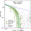 |
Fig. 2. Rest-frame equivalent width of Mg II vs. projected separation of the absorbing galaxy. Black symbols represent direct data from Huang et al. (2021). Olive symbols mark average Wr values weighted by the probability distribution function (PDF) of a Kaplan-Meier estimator of detections and non-detections in the ρ-bin (details in the text). The green line shows the statistical prediction of the |


The above prediction is for κ = 1. The dotted blue line shows  using κ = κ(ρ) in Eq. (7) of Schroetter et al. (2021), also extrapolated to ⟨z⟩. Unsurprisingly, this profile encompasses almost all data points (including upper limits). The few points above the prediction are concentrated at ρ ≲ 70 kpc. In the present approach, these are classified as statistical outliers. We speculate that they may correspond to galaxy-scale processes, e.g., outflows (Weiner et al. 2009; Bradshaw et al. 2013), streams (Waterval et al. 2025), and/or random galaxy orientations that break the spherical symmetry assumed here. Altogether, we conclude that coupling the observational line density and luminosity-function data provides an excellent prediction for the independently observed Wr–ρ data at low redshift; moreover, the luminosity limits used in Eq. (3) naturally yield the correct normalization of
  . Excluding the uncertain weak-Mg II statistics, this finding suggests that most of the strong Mg II is indeed associated with UV-luminous galaxies, with the caveat that quiescent and post-starburst galaxies constitute only a few percent of UV-bright galaxies (e.g., Taylor et al. 2023) in any environment, so their effect (Lan & Mo 2018; Chen et al. 2025) could go unnoticed in our model.
3.2. Redshift dependence
Best-fit results for redshift parametrization of Schechter parameters.
Building on the above procedure, we next investigated Mg II profiles (and hence CGM cross sections) up to the highest redshifts that absorption-line surveys allow. For the UV-galaxy number density, we again applied the parametrization of Bouwens et al. (2021), noting that while mergers are inherently considered in ϕ(z), in the present approach we ignore their possible effect on the absorbing cross sections (Hani et al. 2018). We integrated Eq. 3 from Lmin = 0.01L⋆, corresponding to MB = −16, i.e., the faintest magnitude bin of Bouwens et al. (2021) at z = 6, to Lmax = ∞. To estimate the redshift evolution in f(z, W), we attempted to parametrize in redshift the Schechter parameters reported to fit the still-sparse data for d2N/dzdW. At z < 2, we used the Schechter parameters reported by Mathes et al. (2017, M17) for four redshift bins, correcting their ϕ⋆ to meet our definition of N⋆. At z > 2, to obtain the Schechter parameters, we first re-fit the d2N/dzdW data in the four redshift bins reported by Chen (2017, C17) using a Schechter function (they originally fit an exponential function). We complemented their high-redshift bin with the measurement reported by Bosman et al. (2017, B17). We used a Bayesian approach to explore correlations between parameters and constrain N⋆ such that the area below the Schechter curve equals the total dN/dz of the survey. The results, shown in Fig. A.1, are encouraging and provide robust constraints on W⋆ and α, despite the limited number of data points per redshift bin. With these eight sets of measured Schechter parameters, plus the only other one reported at z > 2 (Sebastian et al. 2024), we explored the redshift evolution using different parametrizations, as shown in Fig. 3. For W⋆, we followed the prescription of Madau & Dickinson (2014), used to fit the evolution of the SFR density. For N⋆ and α, we fit simple power laws. These are functional fits without any particular physical motivation. However, the Madau & Dickinson (2014) parametrization has been used to describe the  data (Zhu & Ménard 2013), which is essentially determined by W⋆ (both in their exponential parametrization and in our Schechter one). The dN/dz peak observed at z ≈ 2 (here seen in W⋆; upper panel of the figure) has already been discussed by various authors and is believed to relate to the peak of cosmic star formation. In fact, the UV luminosity density, needed to obtain the SFR density (e.g., Khusanova et al. 2020), is proportional to the right-hand side of Eq. 3 if β = 0.5; in this case, the proportionality factor is simply L⋆. This suggests that W⋆ should continue to decrease with redshift and that the increase in α is consistent with the anticorrelation between these two parameters, as observed in Fig. A.1. At the same time, N⋆ defines the integral of f(W) and balances the apparent constant line density at high redshift. It remains to be determined whether N⋆ continues to rise beyond z ≈ 6, as forced by the simple function used here, but we argue in Section 5 that this is unlikely.
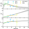 |
Fig. 3. Redshift evolution of the Schechter parameters that fit the d2N/dzdW data from Mathes et al. (2017, M17), Chen (2017, C17), Bosman et al. (2017, B17), and Sebastian et al. (2024, S24). The M17 and S24 data points are published, while the C17 and C17+B17 data points are obtained by us by re-fitting the authors’ d2N/dzdW data (see caption of Fig. A.1). The solid curves are parametrizations of the form y = a(1 + z)b/(1 + ((1 + z)/c)d) fit to the W⋆ data, and y = a(1 + z)b fit to the N⋆ and the α data. The best-fit parameters are listed in Table 1. The 1-σ bands are computed using bootstrapping over the data (W⋆) and covariance-based bootstrapping over the fit parameters (N⋆ and α). |
4. Results
With the redshift parametrizations of f(z, W) we can now make various statistical predictions. First, in Fig. 4, we show redshift snapshots of the Mg II radial profile (κ = 1). The redshifts are selected for comparison with the few available Wr-ρ measurements at z > 2 (Bouché et al. 2012; Møller & Christensen 2020; Bordoloi et al. 2024), and with three redshifts with d2N/dzdW data on neutral oxygen (Becker et al. 2019), for which we can apply our formalism. The Mg II data points are moderately consistent with our statistical prediction, but more data are needed to make a similar comparison to the low-z one in Section 3.1. Unfortunately, there are currently no observational data on Wr1302 versus ρ to independently validate our model on O I. However, a comparison between model predictions for O I and Mg II is worthwhile. In self-shielded neutral gas, O I closely follows H I (e.g., Keating et al. 2014) and has been proposed as a tracer of the H I neutral fraction (Becker et al. 2019; Doughty & Finlator 2019). In contrast, Mg II can occur in both neutral and ionized gas. Therefore, a comparison of the radial profiles of these two species offers good prospects for tracing the growth of metal-enriched bubbles in the pre-reionized IGM. Focusing on Wr2796 > 0.3 Å Mg II and Wr1302 > 0.1 Å O I (where f(W) is still complete), just after reionization (z ∼ 6), our statistical comparison shows that the two ions trace each other similarly, whereas at lower redshifts O I is less extended than Mg II. This is most likely due to ionization effects, since Mg II can survive under slightly higher ionization conditions (and not due to evolution in enrichment of the CGM; Doughty & Finlator 2019). We analyze this scenario in more detail in Section 5.
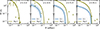 |
Fig. 4. Redshift snapshots of the predicted equivalent-width profiles, |

A more general evolutionary view is shown in Fig. 5, which displays for our Mg II model: (a) the predicted redshift evolution of the comoving line density3, dN/dX, in three Wr intervals; (b) the luminosity-weighted space density of galaxies, ⟨n⟩L; (c) the radius, R, (for κ = 1); and (d) the volume filling factor, defined here as
 (6)
(6)
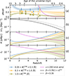 |
Fig. 5. Redshift evolution of various model quantities, shown as following from top to bottom. Panel (a): Statistical prediction of the Mg II comoving line density dN/dX for three cuts in Wr2796 chosen to match published data (colored lines). Data points with the same color codes are from Sebastian et al. (2024) and Chen (2017). Panel (b): Observed L > 0.01L⋆ luminosity-weighted space density of UV-bright galaxies (Bouwens et al. 2021) shown for both fixed and evolving β. Panel (c): Statistical prediction of the Mg II halo radius. Panel (d): Same as panel (c) but for the volume filling factor. Since Wr is binned, both R and fV are averages. The magenta line in panels (a), (c), and (d) represents a constant-velocity wind starting at the Big Bang. Model uncertainties are propagated from those of f and ϕ. A non-evolving β would shift ⟨n⟩L upward by a factor of ≈3, and shift R and fV downward by ≈1.7 and ≈5, respectively. |
In panel (a), the selected Wr intervals enable comparison with the binned data reported in the literature, i.e., Chen (2017) and Sebastian et al. (2024). Since these constrain the d2N/dzdW data used in Section 3, it is not surprising that they capture the predicted evolution in dN/dX. From z ≈ 6 to z ≈ 2, the line density of Wr2796 > 1 Å absorbers steadily increases with time by a factor of ∼3, as noted in (Matejek & Simcoe 2012; Zhu & Ménard 2013; Chen 2017). This is in agreement with our discussion above on W⋆(z), since dN/dX(Wr > 1 Å) is dominated by W⋆. In contrast, the line density of weak absorbers (Wr < 0.3 Å) decreases with time in the same redshift interval. We speculate that this could be due to the complete transmission of ionizing photons upon reionization, which affects the outermost layers of the model (i.e., weak systems) more strongly than the more self-shielded inner layers (i.e., strong systems). The onset of a hard ionizing UV background (UVB) has been linked to the evolution of the ratio of low to high ions upon reionization (Finlator et al. 2016; Becker et al. 2019; Cooper et al. 2019; D’Odorico et al. 2022), although radiation-driven outflows can also remove gas from the low-ionization phase, and these may be more common in the early Universe (Ferrara 2024). Together with a steady increase in the galaxy space density with time, panel (c) shows how these effects are reflected in a 2.5-fold decrease in the radial extent of weak Mg II gas, but only a 1.5-fold for very strong Mg II gas. Hence, the end of reionization could be largely governed by a balance between the growth of metal-enriched, supernova-driven bubbles and regions of photoionized hydrogen, with the former growing more slowly than the latter.
At z ≈ 6, the average proper distance between L > 0.01L⋆ galaxies is ∼2 Mpc, a factor of ≈10 larger than the Mg II radius predicted here for the unity covering fraction, κ = 1. Winds apparently have not been able to reach neighboring halos. This is reflected in the predicted low filling factor, fV ≲ 1 %, and is consistent with theory (e.g.,, Tie et al. 2022; Madau et al. 2001). For the enriched halos to have a linear extent ten times larger, and therefore be able to reach their neighbors, κ ≈ 0.01 would be required (Eq. (4)). In this case, however, the cross section for absorption would be very low (much lower than observed at z ∼ 1; e.g., Schroetter et al. 2021), and consequently the “crossing probability” would also be low. We therefore conclude that, at the end of reionization, the winds have not yet reached the neighboring halos. This implies that halos have so far been mostly self-enriching, as suggested by semi-analytical models (Ventura et al. 2024), in a process mixed with the steady replenishment of IGM material (Waterval et al. 2025).
Our results depend on the chosen parametrization of f(z, W), and in Section 5 we argue that it cannot be extrapolated much beyond z ≈ 6–8. The uncertainty of the model is dominated by that in the f(z, W) parametrization. Regarding the halo-size-luminosity scaling, an unlikely non-evolving β = 0.35 shifts ⟨n⟩L upward by a factor of ≈3 (without affecting the comparison between weak and strong absorbers), and R and fV downward by factors of ≈1.7 and ≈5, respectively, which strengthens the prediction of a low filling factor.
5. Discussion
Within and beyond the reionization epoch in redshift, this regime remains largely uncharted. According to our prediction, the average metal extent beyond z = 6 continuously increases with redshift. However, this contradicts early chemical enrichment models, in which metal-enriched bubbles expand over time (e.g., Furlanetto & Loeb 2003; Wang et al. 2012; Finlator et al. 2020; Yamaguchi et al. 2023). In panels (a), (c), and (d) of Fig. 5, the magenta lines show a toy model in which constant-velocity isotropic winds have expanded around all halos since the Big Bang. Here we use v = 200 km s−1, which is well above the maximum velocity for any dark-matter halo mass in wind models (e.g., Furlanetto & Loeb 2003; Yamaguchi et al. 2023). Thus, this simple wind model sets a firm upper bound for the extent of metals before reionization is complete. It also suggests that a high-redshift extrapolation of our predictions does not hold and that a sharp decline in dN/dX should be observed beyond z = 6–8.
Analytical models (e.g., Furlanetto & Loeb 2003) and hydrodynamical simulations (e.g., Oppenheimer & Davé 2008; Keating et al. 2016; Finlator et al. 2020; Ocvirk et al. 2020) predict that the sizes of the metal-enriched regions (a few pkpc) and thus their volume filling factors, are significantly smaller than those of ionized bubbles (hundreds of pkpc). This results from differences in the mechanisms driving their expansion (mechanical feedback by winds and supernovae and stalled expansion due to metal cooling in the first case, versus radiative feedback in the second; e.g., Madau et al. 2001). As a result, the metal-enriched bubbles expand in an already ionized medium (e.g., Shin et al. 2008) and have a complex, stratified ionization structure (Oppenheimer et al. 2009; Furlanetto & Oh 2005). This complexity has made it difficult for simulations to simultaneously reproduce dN/dX for species probing different ionization states.
Our model predicts an evolution in redshift toward more similar profiles of strong Mg II and O I (Fig. 4), whereas a simple expanding wind model suggests a decreasing line density for both ions. The question arises as to whether these two predictions are consistent with each other. The first prediction is consistent with covering fraction arguments. Such high Wr values are only reached if multiple optically thick clouds are intercepted by the line of sight. This is corroborated by the large number of absorption components typically observed in such high-Wr systems and by numerical simulations, in which neutral gas clouds in expanding outflows have sizes of at most a few hundred parsecs (e.g., Dutta et al. 2025), small compared to the extent of the winds, which reach at least kiloparsec scales (Yamaguchi et al. 2023; Finlator et al. 2020). Therefore, the absorption cross section, and thus dN/dX, is dominated by the projected extent over which multiple optically thick clouds are present in an otherwise ionized volume-filling phase. Each cloud may have a partially ionized outer layer containing only Mg II and no O I (analogous to classical photodissociation regions); however, in a swarm of clouds with high covering fraction, this layer will not dominate the Mg II+O I cross section, leading to similar radial profiles for both ions. By the end of reionization, the rising ionizing background (e.g., Davies et al. 2024) fundamentally alters this scenario. Neutral clouds in the outer parts of the halo become depleted in O I, whereas Mg II can survive more easily. This change in the source of ionizing photons, coupled with the dramatic increase in halo number density, is consistent with the second prediction, and together both factors support the evolutionary trends shown in Figures 4 and 5.
6. Conclusions
Our considerations, based on observational data, assumptions about the halo geometry, and theoretical models of early metal enrichment, predict a complete evolutionary pathway for low-ionization metal-enriched halos. Specifically, we observe a marked difference between the strong and weak Mg II systems. At any redshift upon reionization, strong systems have consistently exhibited a lower incidence (and therefore also a smaller cross section) than weak systems. However, both types of system grow during the first few Myr and peak between z ≈ 8 and 6. After reionization is complete, the incidence of strong systems, coupled with steadily increasing star formation, increases, reaching a peak at cosmic noon. The incidence of weak systems, because they are more exposed to the ambient UVB, steadily decreases or remains constant until it turns over at cosmic noon. By the end of reionization, the metals have not yet reached the neighboring halos. Furthermore, the increase in halo number density causes the average linear extent of both the strong and weak Mg II halos to decrease over time, with the latter decreasing more rapidly. In our model, these evolutionary paths result from the competing effects of increasing halo number density, expanding metal-rich bubbles, and changing ionizationconditions.
We propose that the present approach can continue to be used as new high-redshift campaigns are implemented (e.g., Bordoloi et al. 2024). Galaxy and absorption-line surveys are established techniques with well-known selection functions. Quasars and gamma-ray bursts are already being identified beyond z ≈ 8 and will soon be within reach of JWST and ELT medium-resolution spectroscopy. The identification of intrinsically strong metal transitions, unaffected by the Gunn-Peterson trough, appears feasible down to weak limits in the bright continua of such sources.
The “differential absorption path length” term (Bahcall & Peebles 1969), dX/d , accounts for the cosmological change in the probability of intersection.
Alternatively, Eq. (2) leads to a non-linear differential equation of the form dW + Cf(W)−12πκ(ρ)ρdρ = 0, where C > 0 is a constant.
dN/dX is obtained by integrating Eq. (5) and dividing by dX/dz to remove the cosmological effect on the line density.
Acknowledgments
We thank the anonymous referee for their valuable criticisms. This work has benefited greatly from conversations with Hsiao-Wen Chen, Lise Christensen, Valentina D’Odorico, and Claudio Lopez-Fernandez. S.L. acknowledges support by FONDECYT grant 1231187.
References
- Bahcall, J. N., & Peebles, P. J. E. 1969, ApJ, 156, L7 [NASA ADS] [CrossRef] [Google Scholar]
- Becker, G. D., Pettini, M., Rafelski, M., et al. 2019, ApJ, 883, 163 [NASA ADS] [CrossRef] [Google Scholar]
- Berg, T. A. M., Afruni, A., Ledoux, C., et al. 2025, A&A, 693, A200 [NASA ADS] [CrossRef] [EDP Sciences] [Google Scholar]
- Bolton, J. S., & Haehnelt, M. G. 2013, MNRAS, 429, 1695 [Google Scholar]
- Bordoloi, R., Lilly, S. J., Knobel, C., et al. 2011, ApJ, 743, 10 [CrossRef] [Google Scholar]
- Bordoloi, R., Simcoe, R. A., Matthee, J., et al. 2024, ApJ, 963, 28 [NASA ADS] [CrossRef] [Google Scholar]
- Bosman, S. E. I., Becker, G. D., Haehnelt, M. G., et al. 2017, MNRAS, 470, 1919 [NASA ADS] [CrossRef] [Google Scholar]
- Bouché, N., Murphy, M. T., Péroux, C., et al. 2012, MNRAS, 419, 2 [CrossRef] [Google Scholar]
- Bouwens, R. J., Oesch, P. A., Stefanon, M., et al. 2021, AJ, 162, 47 [NASA ADS] [CrossRef] [Google Scholar]
- Bradshaw, E. J., Almaini, O., Hartley, W. G., et al. 2013, MNRAS, 433, 194 [NASA ADS] [CrossRef] [Google Scholar]
- Carniani, S., Venturi, G., Parlanti, E., et al. 2024, A&A, 685, A99 [NASA ADS] [CrossRef] [EDP Sciences] [Google Scholar]
- Chen, H.-W. 2017, Astrophys. Space Sci. Libr., 434, 291 [Google Scholar]
- Chen, H.-W., Lanzetta, K. M., Webb, J. K., & Barcons, X. 1998, ApJ, 498, 77 [Google Scholar]
- Chen, H.-W., Lanzetta, K. M., & Fernández-Soto, A. 2000, ApJ, 533, 120 [Google Scholar]
- Chen, H.-W., Lanzetta, K. M., & Webb, J. K. 2001, ApJ, 556, 158 [NASA ADS] [CrossRef] [Google Scholar]
- Chen, H.-W., Helsby, J. E., Gauthier, J.-R., et al. 2010a, ApJ, 714, 1521 [NASA ADS] [CrossRef] [Google Scholar]
- Chen, H.-W., Wild, V., Tinker, J. L., et al. 2010b, ApJ, 724, L176 [NASA ADS] [CrossRef] [Google Scholar]
- Chen, Z., Wang, E., Zou, H., et al. 2025, ApJ, 981, 81 [Google Scholar]
- Cherrey, M., Bouché, N. F., Zabl, J., et al. 2025, A&A, 694, A117 [NASA ADS] [CrossRef] [EDP Sciences] [Google Scholar]
- Churchill, C. W., Steidel, C. C., & Vogt, S. S. 1996, ApJ, 471, 164 [Google Scholar]
- Churchill, C. W., Rigby, J. R., Charlton, J. C., & Vogt, S. S. 1999, ApJS, 120, 51 [NASA ADS] [CrossRef] [Google Scholar]
- Churchill, C. W., Mellon, R. R., Charlton, J. C., et al. 2000, ApJS, 130, 91 [NASA ADS] [CrossRef] [Google Scholar]
- Codoreanu, A., Ryan-Weber, E. V., Crighton, N. H. M., et al. 2017, MNRAS, 472, 1023 [NASA ADS] [CrossRef] [Google Scholar]
- Cooper, T. J., Simcoe, R. A., Cooksey, K. L., et al. 2019, ApJ, 882, 77 [CrossRef] [Google Scholar]
- Das, S., Joshi, R., Chaudhary, R., et al. 2025, A&A, 695, A207 [NASA ADS] [CrossRef] [EDP Sciences] [Google Scholar]
- Davidson-Pilon, C. 2019, J. Open Source Software, 4, 1317 [NASA ADS] [CrossRef] [Google Scholar]
- Davies, F. B., Bosman, S. E. I., Gaikwad, P., et al. 2024, ApJ, 965, 134 [NASA ADS] [CrossRef] [Google Scholar]
- D’Odorico, V., Finlator, K., Cristiani, S., et al. 2022, MNRAS, 512, 2389 [CrossRef] [Google Scholar]
- Doughty, C., & Finlator, K. 2019, MNRAS, 489, 2755 [NASA ADS] [CrossRef] [Google Scholar]
- Dutta, R., Fumagalli, M., Fossati, M., et al. 2020, MNRAS, 499, 5022 [CrossRef] [Google Scholar]
- Dutta, A., Sharma, P., & Gronke, M. 2025, MNRAS, submitted [arXiv:2506.08545] [Google Scholar]
- Feigelson, E. D., & Nelson, P. I. 1985, ApJ, 293, 192 [NASA ADS] [CrossRef] [Google Scholar]
- Ferrara, A. 2024, A&A, 684, A207 [NASA ADS] [CrossRef] [EDP Sciences] [Google Scholar]
- Ferrara, A., Pettini, M., & Shchekinov, Y. 2000, MNRAS, 319, 539 [Google Scholar]
- Finlator, K., Oppenheimer, B. D., Davé, R., et al. 2016, MNRAS, 459, 2299 [NASA ADS] [Google Scholar]
- Finlator, K., Doughty, C., Cai, Z., & Díaz, G. 2020, MNRAS, 493, 3223 [NASA ADS] [CrossRef] [Google Scholar]
- Furlanetto, S. R., & Loeb, A. 2003, ApJ, 588, 18 [Google Scholar]
- Furlanetto, S. R., & Oh, S. P. 2005, MNRAS, 363, 1031 [Google Scholar]
- Furlanetto, S. R., Zaldarriaga, M., & Hernquist, L. 2004, ApJ, 613, 1 [NASA ADS] [CrossRef] [Google Scholar]
- Fynbo, J. P. U., Prochaska, J. X., Sommer-Larsen, J., Dessauges-Zavadsky, M., & Møller, P. 2008, ApJ, 683, 321 [NASA ADS] [CrossRef] [Google Scholar]
- Guillemin, P., & Bergeron, J. 1997, A&A, 328, 499 [NASA ADS] [Google Scholar]
- Guo, Y., Bacon, R., Bouché, N. F., et al. 2023, Nature, 624, 53 [NASA ADS] [CrossRef] [Google Scholar]
- Hani, M. H., Sparre, M., Ellison, S. L., Torrey, P., & Vogelsberger, M. 2018, MNRAS, 475, 1160 [CrossRef] [Google Scholar]
- Heckman, T. M., Lehnert, M. D., Strickland, D. K., & Armus, L. 2000, ApJS, 129, 493 [Google Scholar]
- Hogg, D. W. 1999, ArXiv e-prints [arXiv: astro-ph/9905116] [Google Scholar]
- Huang, Y.-H., Chen, H.-W., Shectman, S. A., et al. 2021, MNRAS, 502, 4743 [NASA ADS] [CrossRef] [Google Scholar]
- Kacprzak, G. G., & Churchill, C. W. 2011, ApJ, 743, L34 [Google Scholar]
- Kacprzak, G. G., Churchill, C. W., Steidel, C. C., & Murphy, M. T. 2008, AJ, 135, 922 [NASA ADS] [CrossRef] [Google Scholar]
- Kashino, D., Lilly, S. J., Matthee, J., et al. 2023, ApJ, 950, 66 [CrossRef] [Google Scholar]
- Keating, L. C., Haehnelt, M. G., Becker, G. D., & Bolton, J. S. 2014, MNRAS, 438, 1820 [Google Scholar]
- Keating, L. C., Puchwein, E., Haehnelt, M. G., Bird, S., & Bolton, J. S. 2016, MNRAS, 461, 606 [NASA ADS] [CrossRef] [Google Scholar]
- Khusanova, Y., Le Fèvre, O., Cassata, P., et al. 2020, A&A, 634, A97 [NASA ADS] [CrossRef] [EDP Sciences] [Google Scholar]
- Krogager, J.-K., Møller, P., Christensen, L. B., et al. 2020, MNRAS, 495, 3014 [NASA ADS] [CrossRef] [Google Scholar]
- Lan, T.-W., & Mo, H. 2018, ApJ, 866, 36 [NASA ADS] [CrossRef] [Google Scholar]
- Lanzetta, K. M., Wolfe, A. M., Turnshek, D. A., et al. 1991, ApJS, 77, 1 [Google Scholar]
- Lopez, S., Tejos, N., Ledoux, C., et al. 2018, Nature, 554, 493 [NASA ADS] [CrossRef] [Google Scholar]
- Lundgren, B. F., Creech, S., Brammer, G., et al. 2021, ApJ, 913, 50 [NASA ADS] [CrossRef] [Google Scholar]
- Madau, P., & Dickinson, M. 2014, ARA&A, 52, 415 [Google Scholar]
- Madau, P., Ferrara, A., & Rees, M. J. 2001, ApJ, 555, 92 [Google Scholar]
- Matejek, M. S., & Simcoe, R. A. 2012, ApJ, 761, 112 [NASA ADS] [CrossRef] [Google Scholar]
- Mathes, N. L., Churchill, C. W., & Murphy, M. T. 2017, ArXiv e-prints [arXiv:1701.05624] [Google Scholar]
- Miralda-Escudé, J., & Rees, M. J. 1998, ApJ, 497, 21 [Google Scholar]
- Møller, P., & Christensen, L. 2020, MNRAS, 492, 4805 [CrossRef] [Google Scholar]
- Moster, B. P., Somerville, R. S., Maulbetsch, C., et al. 2010, ApJ, 710, 903 [Google Scholar]
- Nielsen, N. M., Churchill, C. W., & Kacprzak, G. G. 2013, ApJ, 776, 115 [NASA ADS] [CrossRef] [Google Scholar]
- Nielsen, N. M., Churchill, C. W., Kacprzak, G. G., Murphy, M. T., & Evans, J. L. 2015, ApJ, 812, 83 [NASA ADS] [CrossRef] [Google Scholar]
- Ocvirk, P., Aubert, D., Sorce, J. G., et al. 2020, MNRAS, 496, 4087 [NASA ADS] [CrossRef] [Google Scholar]
- Oppenheimer, B. D., & Davé, R. 2008, MNRAS, 387, 577 [NASA ADS] [CrossRef] [Google Scholar]
- Oppenheimer, B. D., Davé, R., & Finlator, K. 2009, MNRAS, 396, 729 [Google Scholar]
- Rubin, K. H. R., Diamond-Stanic, A. M., Coil, A. L., Crighton, N. H. M., & Moustakas, J. 2018, ApJ, 853, 95 [NASA ADS] [CrossRef] [Google Scholar]
- Schroetter, I., Bouché, N. F., Zabl, J., et al. 2021, MNRAS, 506, 1355 [NASA ADS] [CrossRef] [Google Scholar]
- Sebastian, A. M., Ryan-Weber, E., Davies, R. L., et al. 2024, MNRAS, 530, 1829 [NASA ADS] [CrossRef] [Google Scholar]
- Seyffert, E. N., Cooksey, K. L., Simcoe, R. A., et al. 2013, ApJ, 779, 161 [NASA ADS] [CrossRef] [Google Scholar]
- Shapiro, P. R., Giroux, M. L., & Babul, A. 1994, ApJ, 427, 25 [Google Scholar]
- Shin, M.-S., Trac, H., & Cen, R. 2008, ApJ, 681, 756 [Google Scholar]
- Steidel, C. C. 1995, in QSO Absorption Lines, ed. G. Meylan, 139 [Google Scholar]
- Taylor, E., Almaini, O., Merrifield, M., et al. 2023, MNRAS, 522, 2297 [NASA ADS] [CrossRef] [Google Scholar]
- Tie, S. S., Hennawi, J. F., Kakiichi, K., & Bosman, S. E. I. 2022, MNRAS, 515, 3656 [Google Scholar]
- Tinker, J. L., & Chen, H.-W. 2008, ApJ, 679, 1218 [NASA ADS] [CrossRef] [Google Scholar]
- Tinker, J. L., & Chen, H.-W. 2010, ApJ, 709, 1 [Google Scholar]
- Tumlinson, J., Peeples, M. S., & Werk, J. K. 2017, ARA&A, 55, 389 [Google Scholar]
- Ventura, E. M., Qin, Y., Balu, S., & Wyithe, J. S. B. 2024, MNRAS, 529, 628 [Google Scholar]
- Wang, F. Y., Bromm, V., Greif, T. H., et al. 2012, ApJ, 760, 27 [NASA ADS] [CrossRef] [Google Scholar]
- Waterval, S., Cannarozzo, C., & Macciò, A. V. 2025, MNRAS, 537, 2726 [Google Scholar]
- Weiner, B. J., Coil, A. L., Prochaska, J. X., et al. 2009, ApJ, 692, 187 [Google Scholar]
- Weng, S., Péroux, C., Ramesh, R., et al. 2024, MNRAS, 527, 3494 [Google Scholar]
- Whitler, L., Stark, D. P., Topping, M. W., et al. 2025, ApJ, submitted [arXiv:2501.00984] [Google Scholar]
- Willott, C. J., Desprez, G., Asada, Y., et al. 2024, ApJ, 966, 74 [NASA ADS] [CrossRef] [Google Scholar]
- Wolfe, A. M., Turnshek, D. A., Smith, H. E., & Cohen, R. D. 1986, ApJS, 61, 249 [NASA ADS] [CrossRef] [Google Scholar]
- Yamaguchi, N., Furlanetto, S. R., & Trapp, A. C. 2023, MNRAS, 520, 2922 [Google Scholar]
- Zhu, G., & Ménard, B. 2013, ApJ, 770, 130 [NASA ADS] [CrossRef] [Google Scholar]
Appendix A: Schechter function fits
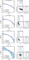 |
Fig. A.1. Schechter function Markov chain Monte Carlo (MCMC) fits to the d2N/dzdW data by Chen (2017, C17). The 6.0 < z < 7.1 bin is complemented with the low-Wr measurement reported by Bosman et al. (2017). The C17 upper limit is treated as a uniform prior truncated at the upper limit value. The fits are constrained such that the area below the fit curve equals the total dN/dz in the exponential fits, i.e., N⋆ in C17. This results in some correlation between the Schechter parameters W⋆ and α. A pure exponential (α = 0) is ruled out at the 1-σ level in three cases. The ± 1-σ confidence band around the fit curve is built from the MCMC samples. |
All Tables
All Figures
|
Fig. 1. Sky-plane representation of a single equivalent width layer illustrating the cases of non-unity (left) and unity covering fraction. |
| In the text | |
|
Fig. 2. Rest-frame equivalent width of Mg II vs. projected separation of the absorbing galaxy. Black symbols represent direct data from Huang et al. (2021). Olive symbols mark average Wr values weighted by the probability distribution function (PDF) of a Kaplan-Meier estimator of detections and non-detections in the ρ-bin (details in the text). The green line shows the statistical prediction of the |
| In the text | |
|
Fig. 3. Redshift evolution of the Schechter parameters that fit the d2N/dzdW data from Mathes et al. (2017, M17), Chen (2017, C17), Bosman et al. (2017, B17), and Sebastian et al. (2024, S24). The M17 and S24 data points are published, while the C17 and C17+B17 data points are obtained by us by re-fitting the authors’ d2N/dzdW data (see caption of Fig. A.1). The solid curves are parametrizations of the form y = a(1 + z)b/(1 + ((1 + z)/c)d) fit to the W⋆ data, and y = a(1 + z)b fit to the N⋆ and the α data. The best-fit parameters are listed in Table 1. The 1-σ bands are computed using bootstrapping over the data (W⋆) and covariance-based bootstrapping over the fit parameters (N⋆ and α). |
| In the text | |
|
Fig. 4. Redshift snapshots of the predicted equivalent-width profiles, |
| In the text | |
|
Fig. 5. Redshift evolution of various model quantities, shown as following from top to bottom. Panel (a): Statistical prediction of the Mg II comoving line density dN/dX for three cuts in Wr2796 chosen to match published data (colored lines). Data points with the same color codes are from Sebastian et al. (2024) and Chen (2017). Panel (b): Observed L > 0.01L⋆ luminosity-weighted space density of UV-bright galaxies (Bouwens et al. 2021) shown for both fixed and evolving β. Panel (c): Statistical prediction of the Mg II halo radius. Panel (d): Same as panel (c) but for the volume filling factor. Since Wr is binned, both R and fV are averages. The magenta line in panels (a), (c), and (d) represents a constant-velocity wind starting at the Big Bang. Model uncertainties are propagated from those of f and ϕ. A non-evolving β would shift ⟨n⟩L upward by a factor of ≈3, and shift R and fV downward by ≈1.7 and ≈5, respectively. |
| In the text | |
|
Fig. A.1. Schechter function Markov chain Monte Carlo (MCMC) fits to the d2N/dzdW data by Chen (2017, C17). The 6.0 < z < 7.1 bin is complemented with the low-Wr measurement reported by Bosman et al. (2017). The C17 upper limit is treated as a uniform prior truncated at the upper limit value. The fits are constrained such that the area below the fit curve equals the total dN/dz in the exponential fits, i.e., N⋆ in C17. This results in some correlation between the Schechter parameters W⋆ and α. A pure exponential (α = 0) is ruled out at the 1-σ level in three cases. The ± 1-σ confidence band around the fit curve is built from the MCMC samples. |
| In the text | |
Current usage metrics show cumulative count of Article Views (full-text article views including HTML views, PDF and ePub downloads, according to the available data) and Abstracts Views on Vision4Press platform.
Data correspond to usage on the plateform after 2015. The current usage metrics is available 48-96 hours after online publication and is updated daily on week days.
Initial download of the metrics may take a while.