| Issue |
A&A
Volume 703, November 2025
|
|
|---|---|---|
| Article Number | A174 | |
| Number of page(s) | 11 | |
| Section | Cosmology (including clusters of galaxies) | |
| DOI | https://doi.org/10.1051/0004-6361/202555729 | |
| Published online | 25 November 2025 | |
An emulator-based forecasting on astrophysics and cosmology with 21 cm and density cross-correlations during the epoch of reionization
Max-Planck-Institut für Astronomie, Königstuhl 17, D-69117 Heidelberg, Germany
⋆ Corresponding author: This email address is being protected from spambots. You need JavaScript enabled to view it.
Received:
29
May
2025
Accepted:
5
September
2025
Abstract
The 21 cm signal arising from fluctuations in the neutral hydrogen field, and its cross-correlation with other tracers of cosmic density, are promising probes of the high-redshift Universe. In this study, we assessed the potential of the 21 cm power spectrum, along with its cross-power spectrum with dark matter density and associated bias, to constrain both astrophysics during the reionization era and the underlying cosmology. Our methodology involves emulating these estimators using an artificial neural network (ANN), enabling efficient exploration of the parameter space. Utilizing a photon-conserving semi-numerical reionization model, we constructed emulators at a fixed redshift (z = 7.0) for k modes relevant to upcoming telescopes such as SKA-Low. We generated ∼7000 training samples by varying both cosmological and astrophysical parameters along with initial conditions, achieving a high accuracy when compared to true simulation outputs. While forecasting, the model involves five free parameters: three cosmological (Ωm, h, σ8) and two astrophysical (ionizing efficiency, ζ, and minimum halo mass, Mmin). Using a fiducial model at the mid-reionization stage, we created a mock dataset and performed forecasting with the trained emulators. Assuming a 5% observational uncertainty combined with emulator error, we find that the 21 cm and 21 cm-density cross-power spectra can constrain the Hubble parameter (h) to better than 6% at a confidence interval of 95%, with tight constraints on the global neutral fraction (QHI). The inclusion of bias information further improves constraints on σ8 (< 10% at 95% confidence). Finally, robustness tests with two alternate ionization states and a variant with higher observational uncertainty show that the ionization fractions are still reliably recovered, even when cosmological constraints weaken.
Key words: cosmological parameters / cosmology: theory / large-scale structure of Universe / dark ages / reionization / first stars
© The Authors 2025
 Open Access article, published by EDP Sciences, under the terms of the Creative Commons Attribution License (https://creativecommons.org/licenses/by/4.0), which permits unrestricted use, distribution, and reproduction in any medium, provided the original work is properly cited.
This article is published in open access under the Subscribe to Open model.
Open Access funding provided by Max Planck Society.
1. Introduction
The Epoch of Reionization (EoR) signifies the last major phase transition in the cosmic history of our Universe, when it evolves from a mostly neutral to a mostly ionized state (for reviews, see the following: Barkana & Loeb 2001; Choudhury 2009; Dayal & Ferrara 2018; Gnedin & Madau 2022; Choudhury 2022). The fluctuation in the neutral hydrogen field during the EoR can potentially be traced by the redshifted 21 cm signal, which arises due to the spin flip transition of the neutral hydrogen atoms at the ground state. The signal carries useful information on cosmological and astrophysical properties of this high-redshift epoch. This can provide comprehensive answers to the questions concerning the ionization and thermal state of the high-redshift intergalactic medium (IGM), the nature of the first ionizing sources, and the timeline of the reionization epoch. It can also inform us about cosmic expansion and structure evolution (Pritchard & Loeb 2012).
While the radio interferometers are gradually improving their sensitivity to detect the 21 cm signal, these still face significant challenges in terms of foreground contamination and instrument characterization, allowing only upper limits on the detection. These efforts include independent groups focussing on different telescopes such as the Low Frequency Array (LOFAR; Gehlot et al. 2019; Mertens et al. 2020, 2025), the Murchison Widefield Array (MWA; Barry et al. 2019; Trott et al. 2020; Nunhokee et al. 2025), the Giant Metrewave Radio Telescope (GMRT; Paciga et al. 2013), and the Hydrogen Epoch of Reionization Array (HERA phase I; HERA Collaboration 2023) at the redshift range z ∼ 6 − 10. A few projects, such as Owens Valley Long Wavelength Array (OVRO-LWA; Eastwood et al. 2019) and New Extension in Nançay Upgrading LOFAR (NenuFAR; Mertens et al. 2021; Munshi et al. 2024), also aim for higher redshifts covering cosmic dawn. The limits have already been exploited to constrain some of the extreme reionization models (Ghara et al. 2025). However, with upcoming facilities such as SKA-Low (AA* and AA4 configuration), we expect to detect the signal with percentage-level uncertainties.
As 21 cm signal is supposed to be mainly driven by astrophysical processes, most of the EoR studies with 21 cm signal as a probe mainly focus on constraining uncertain astrophysical parameters, keeping the underlying cosmology fixed. Nonetheless, 21 cm signal can also play a crucial role in probing cosmology in combination with other probes such as the CMB (McQuinn et al. 2006; Liu & Parsons 2016). However, the studies aiming for cosmological forecasts with 21 cm signal require efficient models to explore astrophysics and cosmology simultaneously. To this end, the analytical halo model of reionization (Schneider et al. 2023) and machine-learning-based techniques (Kern et al. 2017; Hassan et al. 2020) have recently been exploited, highlighting the prospects of constraining cosmology and astrophysics with 21 cm. Specifically, the approach of creating emulators of observables or likelihoods has been reasonably successful in inferring astrophysical parameters from 21 cm power spectra and EoR observables (Shimabukuro & Semelin 2017; Schmit & Pritchard 2018; Maity et al. 2023; Breitman et al. 2024; Sikder et al. 2024; Choudhury et al. 2024, 2025).
In parallel, windows are now opening up for synergetic studies with 21 cm and other high-redshift probes. For example, the distribution of Ly-α-emitting high-redshift galaxies can be used as a biased tracer of large-scale density structure of the Universe and is useful for cross-correlation with 21 cm (Vrbanec et al. 2016; La Plante et al. 2023; Moriwaki et al. 2024). Other tracers of density exist, such as intensity maps (for a review, see Kovetz et al. 2017) of CO (Lidz et al. 2011), CII (Gong et al. 2012), Hα (Heneka & Cooray 2021), OIII (Moriwaki et al. 2018), and near-infrared background (Sun et al. 2025), which can also be utilized for cross-correlation studies. Hence, the cross-correlation between 21 cm and cosmic-matter density, an estimator independent of any specific tracers, can provide us with a potential probe of the high-redshift Universe (Xu et al. 2019). Furthermore, the cross-power spectra is a superior probe in terms of signal-to-noise ratio due to uncorrelated systematics and can complement the pure 21 cm auto-power spectrum signal. With the availability of current and upcoming telescopes such as the James Webb Space Telescope (JWST), Nancy Grace Roman Space Telescope (NGRST), Extremely Large Telescope (ELT), and so on, the cross-correlation prospects have been shown to be promising for gleaning astrophysical signal during the EoR (Gagnon-Hartman et al. 2025). In principle, the cross-correlation information can also be utilized to infer cosmology, which has already been explored in low-redshift studies (Berti et al. 2024; Autieri et al. 2025).
In this study, we aim to check the prospects of 21 cm and its cross-correlation information with matter density in constraining both astrophysics and cosmology during the reionization epoch. Unlike other semi-numerical approaches based on the excursion set algorithm, we utilized a more realistic prescription provided by the Semi Numerical Code for ReIonization with PhoTon Conservation (SCRIPT) to generate the neutral hydrogen fluctuation field. We only considered a single redshift (z = 7.0) for creating the emulators and pursuing parameter exploration, which gives us a starting point as a proof of concept. However, this can be extended to multiple redshifts, exploring the full power of 21 cm observables in future studies.
The paper is organized as follows. In Section 2, we describe the reionization model and define the observables (or estimators) explored. Next, we discuss building the emulators of those observables, highlighting the performance of our emulators against the true values in Section 3. Once the emulator is trained, we describe the mock generation procedure in Section 4 and parameter exploration in Section 5. Then, we discuss our main results in Section 6. Finally, we summarize the paper in Section 7.
2. Reionization model, observables, and estimators
The reionization models implemented in SCRIPT were originally introduced by Choudhury & Paranjape (2018) and have since been exploited with various observables (Maity & Choudhury 2022a,b). In this work, we adopted the simplest version of this framework – a two-parameter reionization model previously used for 21 cm forecasting (Maity & Choudhury 2023). For completeness, we briefly summarize the methodology in the following.
The SCRIPT code simulates the ionization state of the Universe within a cosmologically representative volume, enabling the computation of large-scale ionization fluctuation power spectra that are converged with respect to the resolution of the simulation box (Choudhury & Paranjape 2018). To initialize the model, we provide the density field and the spatial distribution of collapsed halos capable of emitting ionizing radiation. Focusing on large-scale IGM features, we used the second-order Lagrangian perturbation theory (2LPT) to generate the density field, rather than relying on computationally expensive full N-body simulations. Specifically, we used the implementation by Hahn & Abel (2011)1. This model also allows us to vary different cosmological parameters (Ωm, h, σ8, ns, and w0 in this case) as well as the initial seed for generating the fluctuating fields. The parameters have the standard meanings, i.e., Ωm is dark matter density; h is the hubble parameter; σ8 quantifies the amplitude of primordial matter fluctuations; ns is the tilt of the primordial power spectra; and w0 is the dark energy equation of state. We fixed the baryonic density parameter (Ωb = 0.0482) throughout the study. The distribution of halos was computed using a subgrid approach based on the conditional ellipsoidal collapse mass function (Sheth & Tormen 2002). Although this approach has been proven to be extremely successful for standard Λ-Cold Dark Matter (ΛCDM) models, one essential assumption for our study is that the prescription remains the same for the range of cosmology models considered here. Simulations are conducted within a comoving box of 256 h−1 cMpc, which has been shown to be sufficient for the observables considered here, as demonstrated in recent literature (Iliev et al. 2014; Kaur et al. 2020). The spatial resolution is set to Δx = 2 h−1 cMpc, which is adequate for capturing the scales accessible to SKA-Low.
As mentioned earlier, we used a basic reionization model containing two free parameters, which are needed to obtain the ionization topology. The model adopts the photon-conserving algorithm to construct the reionization topology within the simulation box. Specifically, the ionization field relies on the ionization efficiency parameter (ζ), which estimates the available ionizing photons per hydrogen atom and minimum threshold halo mass (Mmin) required to obtain the fraction of mass collapsed inside a halo. We restricted ourselves to this simple two-parameter setup as we aim to pursue a prospective forecasting study with 21 cm and its cross-correlations with matter density, while simultaneously varying astrophysical and cosmological parameters. This basic setup helps us to gain the required efficiency by minimizing the parameter space. However, the study can be expanded with more physical models of reionization, including recombination and radiative feedback effects (Maity & Choudhury 2022a) in a future project.
In general, any model of reionization produces the ionized hydrogen fraction of xHII, i in grid cells (represented by the index i) inside a simulation volume. The differential brightness temperature (assuming spin temperature is much larger than CMB temperature) is then given by (Madau et al. 1997; Ciardi & Madau 2003)
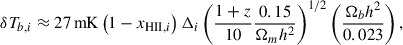 (1)
(1)
where  is the ratio of the matter density ρm, i in the grid cell and the mean matter density
  .
.
Given these quantities, the 21 cm power spectrum can be computed as
 (2)
(2)
where  is the Fourier transform of the mean-subtracted normalized fluctuation field, δTb, i/⟨δTb, i⟩−1.
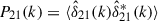
Similarly, the cross-power spectra between the 21 cm field and the matter density field are given by
 (3)
(3)
where  is the Fourier transform of matter density contrast (Δi − 1). It is worth highlighting that 21 cm-density cross-power spectrum cannot be observed directly by any tracers, but these can be derived by observing galaxy distribution and estimating galaxy bias with respect to the background dark matter distribution. With the assumption of linear galaxy bias, galaxy density is essentially proportional to the matter density (La Plante et al. 2023). The linear bias is expected to be a reasonable approximation for the large-scale modes, which are of interest in this study. Hence, 21 cm, along with high-redshift galaxy surveys, can be utilized as a direct probe of the cross-correlation. For simplification, we use the term observables even for the indirect estimators unless otherwise specified. Throughout the study, we worked with dimensionless power spectra which are given by
 (4)
(4)
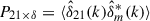
where PX corresponds to the different power spectra (P21, P21 × δ) as defined earlier. The 21 cm field and the density field are supposed to be highly anti-correlated at large scales, providing negative cross-power. This is expected due to the efficient ionization of high density regions, forming the ionizing sources, and similarly, less efficient ionization at low density regions. Hence, we used the amplitude of cross-power spectra (|Δ21 × δ2|) as the probe in this study (see also Moriwaki et al. 2024). We can further define the bias of the 21 cm-density cross-power spectrum with respect to matter power spectrum (Pδδ) as
 (5)
(5)
This is relatively easy to estimate due to uncorrelated systematics in the cross-spectra compared to the bias of 21 cm auto-power spectra. Hence, we chose this probe instead of the bias of the auto-power spectra. We also quantified the state of the IGM by globally averaged neutral fraction, QHI = ⟨(1 − xHII, i)Δi⟩. As discussed earlier, we aim to check the prospects of these observables in constraining astrophysical parameters relevant for EoR as well as inferring the underlying cosmological model. This further demands efficient methods of computation, which are discussed in the next section.
3. Emulating the observables and estimators
In order to pursue parameter space exploration, we constructed an emulator that can predict the observables given a set of parameters. In this study, we initially had two astrophysical parameter (ζ, Mmin), defining reionization models and five cosmological parameters (Ωm, h, σ8, ns, w0). However, we fixed ns and w0 at standard values while pursuing parameter exploration, as these are not expected to substantially affect the scales and the redshifts considered here. Hence, we continued with rest of the three cosmological parameters, acquiring efficiency. The next aim was to predict the observable values given the free parameters as inputs. To this end, we utilized a supervised machine learning technique, specifically an artificial neural network (ANN), to train the emulator.
3.1. Artificial neural network in brief
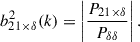
An ANN is composed of an input layer, one or more hidden layers, and an output layer. The input layer receives raw data, while the hidden layers perform complex computations to extract meaningful features. The output layer then provides the final prediction. Each connection between neurons has an associated weight and bias, which are adjusted during the training to minimize errors. Furthermore, in order to allow the network to learn complex patterns, non-linearities are introduced by activation functions such as ReLU and Sigmoid. The learning process is guided by a loss function, which measures the error; and an optimization algorithm such as gradient descent or Adam, which updates the weights through back-propagation (for details, see Bishop & Nasrabadi 2007; Choudhury et al. 2020). A portion of the training datasets were used for validation purposes during the development of the emulator, and this process progresses in an iterative manner. Once the network is fully trained, it is tested on a different set of data, providing a robustness check on the predictions. In general, ANNs can face two key challenges during training; i.e., underfitting and overfitting. Underfitting occurs when the model is too simple to capture the patterns in the data, leading to poor performance on both the training and validation sets. This often happens when the network has too few layers or neurons, or when the training time is insufficient. On the other side, overfitting happens when the model learns the noise and specific details of the training data instead of generalizing to new data. This results in excellent performance on the training set, but poor accuracy on unseen validation or test data. Overfitting is common when the network is too complex or trained for too many epochs without proper regularization. To check the performance of the network, we used an R2 metric score, which is defined as
 (6)
(6)
where ytrue is the true value of the observables from simulation, ⟨ytrue⟩ is the average from the test set, and ypredict is the corresponding prediction from the network. This essentially provides an assessment for goodness of fit, where the metric value can vary from 0 to 1. As the R2 value approaches 1, the prediction capability of the emulator improves.
3.2. Training procedure
To generate the training dataset, we varied the different parameters within reasonable prior ranges; i.e., Ωm : [0.2, 0.4], h : [0.6, 0.8], σ8 : [0.7, 0.9], ns : [0.9, 1.0], w0 : [ − 2, 0], ζ : [1, 40], and log Mmin : [7, 12]. The baryonic density parameter, Ωb is fixed at 0.0482, obeying the findings from CMB spectra (Planck Collaboration VI 2020). We stored the power spectra in 10 different bins from k ≃ 0.05 h/cMpc to 1.084 h/cMpc. However, we only took 6 bins in the k ≃ 0.11 h/cMpc to 0.84 h/cMpc range for further analysis, which are expected to be probed by upcoming instruments such as SKA-Low. The goal here is to predict the corresponding amplitude in those bins given a set of parameter values. Given that motivation, we generated a total of 6750 samples for each type of observable (21 cm power spectra, 21 cm-density cross-power-spectra amplitude and cross-bias) by randomly varying these parameters. Among these samples, 500 correspond to different realizations of the initial seed. This further takes into account the cosmic variance uncertainties during the training. We utilized publicly available Scikit-learn and TensorFlow packages in Python to implement the network. We split the sample into training and testing sets with a ratio of 80–20. Our assumed network architecture is summarized in Table 1. We used ReLU activation between the layers and Adam optimizer in this setup. An architecture with 10 hidden layers along with one input and one output layer, performed well to serve the purpose of the study.
ANN architecture for training the 21 cm power spectra and cross bias.
In Figure 1, we show the comparison between true 21 cm power amplitude against the prediction from the trained network for the test samples. Each panel shows the six different bins considered in this study. It is visually clear that the true and predicted values are well correlated with each other, signifying a good accuracy of the prediction. The overall R2 metric score for the test set is 0.98, which also quantifies a well trained model with high predictive power. Similarly, we show the true-versus-prediction plot for the 21 cm-density cross-power spectrum in Figure 2 and for cross-bias in Figure 3. The corresponding R2 metric values are 0.99 and 0.92, respectively, which again provides a significantly accurate prediction. For cross-power spectra, we emulated the quantity QHI|Δ21 × δ2| at first and then divided by QHI, where the IGM is not fully ionized. This helps us to avoid any possible divergence due to fully ionized IGM in the training set. The scatter at lower amplitudes arises mainly due to the fact that these correspond to highly ionized states of the IGM and hence there is very little leftover correlation information between 21 cm and the density distribution. In Figure 4, we further show the comparison plots of the true model and emulator prediction for the different observables as functions of k modes using six random sets of parameter samples in our test suite. The true (solid) and the predicted (dashed) cases match reasonably well for the different models. This gives us confidence on the emulator’s performance over a wide range of models. In Figure 5, we give an example of a fiducial model which has been discussed in Section 4.
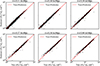 |
Fig. 1. Comparison of true 21 cm power spectrum and corresponding predicted estimates using ANN at different k bins used in this work. The black points correspond to test dataset, while the red line signifies True = Prediction. The corresponding R2 value is 0.98. |
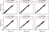 |
Fig. 2. Comparison of true cross-power amplitude between 21 cm and δ m field with the corresponding predicted estimates using ANN at different k bins used in this work. Other descriptions are similar to those of Figure 1. This corresponds to an R2 value of 0.99. |
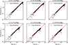 |
Fig. 3. Comparison of true 21 cm bias and the corresponding predicted estimates using ANN at different k bins used in this work. Other descriptions are similar to those of Figure 1. The corresponding R2 value is 0.92. |
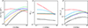 |
Fig. 4. Plots of 21 cm power spectra, 21 cm-density cross-power, and its bias for a few random models from the test set. The solid lines show the true models, while the dashed lines give the corresponding predictions. |
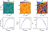 |
Fig. 5. Top panel: Snapshots of density (Δ), collapsed fraction (fcoll), and neutral fraction field (xHI), gradually in order from left to right, for the fiducial model utilized to generate the mock dataset as described in Section 4. Bottom panel: 21 cm power spectra (⟨δT b⟩2 Δ21 2), 21 cm and density cross-power spectra (|Δ21 × δ 2|), and the bias of cross-spectra (b21 × δ 2) for the corresponding model, gradually from left to right. |
We also utilized the datasets to predict the global neutral fraction (QHI), providing the same set of free parameters. Instead of a complex network, a simpler technique using Gaussian process regression (GPR) is sufficient to give a reasonably accurate prediction in this case, corresponding to an R2 metric score of 0.98. In Figure 6, we show the comparison between the true global neutral fraction and the corresponding predictions from GPR. These are nicely correlated with each other along the equality line with an average scatter uncertainty < 5%.
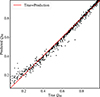 |
Fig. 6. Comparison of true neutral fraction (QHI) and corresponding predicted estimates using Gaussian process regression. |
4. Generating the mock data
We chose a fiducial set of parameters to generate the mock observables. For exploration studies, we fixed ns = 0.961 and w0 = −1, which is consistent with the CMB estimates (Planck Collaboration VI 2020). The rest of the parameter values corresponding to these fiducial mocks were chosen as Ωm = 0.308, h = 0.678, σ8 = 0.829, ζ = 15, and log Mmin = 9.0. The values were shifted by a Gaussian random noise with a standard deviation consistent with the expected level of SKA-Low (AA*) thermal noise with 1000 h of observations. These shifted values are treated as the mock dataset for our analysis. The total errors on the mock dataset are assumed to have two contributions; i.e., training uncertainties (σ𝒟tr) and the overall observational uncertainties (σ𝒟obs). We computed the training uncertainties by quantifying the scatter in true-versus-predicted observable distributions. Specifically, we estimated 84% and 16% quantiles for (true − predicted) distributions and then took half the difference between those two quantiles to obtain σ𝒟tr. For observational uncertainties, we assumed a moderate value of 5% of the observable amplitude at the corresponding k bins. This is motivated by the expected signal-to-noise ratio (≳20) on 21 cm power spectra from SKA-Low AA* observations for 1000 h with an optimistic foreground scenario2. We also show a case with a more conservative uncertainty, assuming 10% of the amplitude. Then, the total uncertainties are estimated by adding these contributions in quadrature as
 (7)
(7)
In the top panels in Figure 5, we show the different cosmological fields, including the matter density (Δ), collapsed fraction (fcoll), and neutral fraction (xHI). The fluctuations in these fields are nicely correlated with each other. In the bottom panels, we show the corresponding observables; i.e., 21 cm power spectra (⟨δTb⟩2Δ212), 21 cm-density cross-power spectra (|Δ21 × δ2|), and bias (b21 × δ2). The black data points with error bars are utilized for the parameter space exploration studies, while the dashed blue line represents the underlying input model. We adopted a conservative approach by using only two k bins with the better prediction uncertainties (among all the 6) for the 21 cm bias, as this has a relatively lower prediction accuracy among the three estimators considered in this study. This helped us to minimize the bias coming from poor emulator predictions.
We continued the study utilizing two variants of the mock dataset using different input models corresponding to different ionization states. These are generated by changing the ζ values appropriately. To ensure robustness, we checked the results with a smaller (ζ = 10) and a larger (ζ = 20) value than the fiducial ones as discussed later in Section 6.
5. Parameter exploration with emulator
We employed a standard Bayesian framework to explore the parameter space of our model. Our objective was to compute the posterior probability distribution, 𝒫(λ|𝒟), of the model parameters, λ, conditioned on the observational (mocks in this case) datasets, 𝒟 introduced in the previous section. According to Bayes’ theorem, the posterior is given by
 (8)
(8)
where ℒ(𝒟|λ) denotes the likelihood, π(λ) represents the prior distribution, and 𝒫(𝒟) is the Bayesian evidence. The evidence serves as a normalization constant and does not influence our parameter inference.
The likelihood function was modeled as a multivariate Gaussian distribution,
![Mathematical equation: $$ \begin{aligned} \mathcal{L} (\mathcal{D} \vert \lambda ) =\exp \left(-\frac{1}{2} \sum _{\alpha }\left[\frac{\mathcal{D} (k_{\alpha })-\mathcal{M} (k_{\alpha }; \lambda )}{\sigma _\mathcal{D} ^{tot}(k_{\alpha })}\right]^2 \right). \end{aligned} $$](/articles/aa/full_html/2025/11/aa55729-25/aa55729-25-eq13.gif) (9)
(9)
Here 𝒟 corresponds to different mock observables or estimators (i.e., ⟨δTb⟩2Δ212, |Δ21 × δ2| and b21 × δ2) and ℳ is the corresponding predictions for parameter set λ.
To sample the posterior distribution, we utilized the Markov Chain Monte Carlo (MCMC) method, employing the Metropolis–Hastings algorithm (Metropolis et al. 1953). The MCMC chains were executed using the publicly available cobaya package (Torrado & Lewis 2021)3. We checked the convergence of the chains following the Gelman-Rubin R − 1 statistic (Gelman & Rubin 1992). The chain was assumed to have converged when the R − 1 value was lower than a threshold of 0.01. For subsequent analysis, we discarded the initial 30% of samples from each chain as burn-in and based our inference on the remaining samples.
6. Results
In this section, we discuss the findings from our parameter space exploration studies using mock datasets. In Table 2, we provide the 95% confidence limits along with mean of the recovered cosmological parameters as well as the ionization state for different scenarios considered in this study.
Parameter constraints obtained from MCMC-based analysis for different scenarios using mock dataset.
In Figure 7, we show the posterior recoveries of the free parameters from the fiducial mock dataset. The free parameters include both cosmological (Ωm, h, σ8) as well as astrophysical ones (ζ, log Mmin). We also show the posterior of the globally averaged neutral fraction (QHI) as a derived parameter. We find that the parameters are not well constrained for the case where we utilize only 21 cm power spectra (shown in red), although it can correctly recover the global neutral fraction with significant uncertainties. The constraints are clearly improved when we include 21 cm-density cross-power spectra as observables along with 21 cm power spectra (shown in lime green). Specifically, the Hubble parameter (h) is constrained within an uncertainty of < 6% at a confidence interval of 95%. This signifies the potential of 21 cm and synergies with galaxy observables as an independent probe to constrain the expansion rate of the universe, which can further shed light on the well-known Hubble tension (Riess et al. 2019; Verde et al. 2019). Furthermore, the global neutral fraction is now stringently constrained, discarding a significant portion of astrophysical parameter spaces. On top of that, if we include the bias of cross-spectra, it further constrains the σ8 parameter (providing < 10% uncertainty at 95% confidence). This happens as the combination now has the information on the amplitude of the underlying matter power spectra (see Equation (5)), which is controlled by σ8. We also note that the reionization source parameters are also well recovered, and the uncertainties subsequently improve as we include more observables. However, Ωm is bounded by only one side due to strong degeneracy with astrophysical parameters.
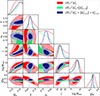 |
Fig. 7. Comparison of posterior distributions using different combinations of observables i.e. only 21 cm power spectra (red), 21 cm power spectra + 21 cm-density cross-power spectra (green), and adding bias of cross-spectra (blue). The diagonal panels show the 1D posterior probability distribution, and the off diagonal panels show the joint 2D posteriors. The contours represent the 68% and 95% confidence intervals. The dashed line represents the input parameter values used to generate the mock dataset. The observational uncertainties are assumed to be 5% of the observable amplitudes in this case. |
To check the robustness of the findings, we further pursued parameter space exploration using two more mock datasets with different ionization states. We tuned the ionizing efficiency parameter to generate the mocks with a higher (QHI = 0.65) and a lower (QHI = 0.29) neutral fraction than the fiducial one (QHI = 0.47), while all the other input parameters are kept the same as before. In Figure 8, we show the recovered posteriors of these cases along with the fiducial one. We find that the h and σ8 parameters are well constrained even for the higher neutral fraction, recovering the underlying true values within a 95% uncertainty level as before. The astrophysical parameters are also consistent with the input values. On the other hand, the constraints on the parameters for the lower neutral fraction are not significantly strong, barely constraining h and providing a one-sided bound on σ8 at a 95% uncertainty level. This is not very surprising as the ionized bubbles start to overlap when the Universe is highly ionized (lower neutral fraction), which can wipe out the correlation information, resulting in a loss of constraining power. However, the neutral fraction was still recovered with significant precision without any strong bias. This also confirms the fact that the 21 cm observables are more sensitive to the ionization state of the Universe rather than the underlying cosmological information.
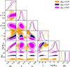 |
Fig. 8. Comparison of posterior distributions for mocks corresponding to different ionization states. Along with the fiducial case (QHI = 0.47, in blue), we show two more cases for a lower (QHI = 0.29, in orange) and a higher neutral fraction (QHI = 0.65, in magenta). The observational uncertainties are assumed to be 5% of the amplitudes, as in Figure 7. |
Lastly, we checked the effects of observational uncertainties on the posterior distribution in Figure 9. The green contours show the case where we assume the uncertainties to be 10% of the observable amplitudes, while the other one is the same as the fiducial case with 5% uncertainties. Not surprisingly, the contour widens for larger uncertainties; however, it still manages to correctly recover the Hubble parameter and amplitude of primordial fluctuations with significant confidence.
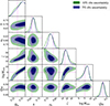 |
Fig. 9. Comparison of posterior distributions for mocks corresponding to different observational uncertainties assumed in the likelihood. The blue contours correspond to the fiducial case with 5% uncertainties, as also shown in Figures 7 and 8; while the green contours correspond to a variant with 10% observational uncertainties for all the observables used. . |
7. Summary and conclusions
The astrophysics during the EoR is gradually being explored with the help of multiwavelength observables. The 21 cm signal is one of the crucial probes that has the potential to detect neutral hydrogen fluctuations at the EoR directly. This further contains useful information about the cosmological parameters, although it is hard to infer cosmology from this weak signal, affected by foreground contamination and poorly understood high redshift astrophysical phenomena. To this end, the cross-correlation of 21 cm signal with other tracers of cosmological density can be a complementary probe of astrophysics and cosmology. This is useful for avoiding any systematics arising due to spurious correlation and, hence, enhancing the signal-to-noise ratio of detection. In this study, we check the prospects of 21 cm-density cross-power and its bias along with 21 cm power spectra in order to probe the astrophysics and cosmology from the EoR. Our approach relies on creating an efficient emulator of the observables and utilizing the emulator for further parameter space exploration. Below, we summarize this work, highlighting the main findings.
-
We used a realistic semi-numerical reionization model based on a photon-conserving algorithm to study the prospects of 21 cm and related observables to infer cosmology and astrophysics during the EoR. Specifically, we used 21 cm auto-power spectra, the magnitude of cross-power between 21 cm fluctuations and matter density, and the corresponding bias magnitude. As a prospective study, we focused on a single redshift (i.e., z = 7.0) in this work. While 21 cm auto-power spectra can be observed directly by the radio interferometers, 21 cm-density cross-power spectra and the bias cannot be measured directly. However, the cross-power and its bias can in principle be estimated by different tracers, especially via galaxy-21 cm cross-correlation. We created a total of ∼7000 samples by varying different astrophysical and cosmological parameters to build the emulator for these observables or estimators. The samples were generated with different initial random seeds, which further takes into account the cosmic-variance uncertainties. The emulators were trained to predict the observables at 6 different k bins, given a set of free parameters (including astrophysical and cosmological ones) as inputs. The bins were chosen in the range where we can expect the detection of 21 cm signal from the upcoming telescopes such as SKA-Low. We compared the emulators against true values and found that the predictions are sufficiently accurate, providing R2 values of > 0.9 for all the cases (0.98 for 21 cm auto-power spectra, 0.99 for cross-power spectra, 0.92 for bias amplitude). This provided us with the confidence to carry out efficient parameter space exploration utilizing the emulators.
-
Next, we generated the mock observables with a fiducial set of parameter values consistent with Planck Collaboration VI (2020) and providing an ionization state close to the middle of the reionization process. We found that 21 cm power spectra alone cannot constrain the cosmological parameters, while they can recover the correct ionization state. When we included cross-power spectra as another observable, the Hubble parameter was constrained, and adding the bias magnitude further constrained the amplitude of primordial matter fluctuations (σ8). Similarly, the constraints on the ionization state were also improved significantly. We further pursued a similar analysis with two more mock datasets corresponding to a higher and lower neutral fraction. The recoveries were degraded for lower neutral fraction due to a possible lack of correlation information. However, the ionization states were still precisely recovered for all the cases.
We would like to caution that the exact quantification of constraints is dependent on the emulator uncertainties, which can be improved with larger datasets spanning wider parameter spaces and with more sophisticated training techniques. We also neglected any covariance between the Fourier modes and between observables while computing the likelihood. While the mutual covariances would be ideal to include and may probably degrade the uncertainties, the estimates of 21 cm observables are generally provided without the covariance information in the literature (Ghara et al. 2025). Similarly, multi-observable inference studies usually neglect covariance information between the observables (Maity & Choudhury 2022b; Qin et al. 2025). Hence, we proceed with the diagonal terms, assuming relatively conservative uncertainties and mutually independent observables. Further, one needs to be cautious while interpreting cosmology with real observational data, as the observational estimates (limits till now) are often derived assuming an underlying cosmology, which should be properly quantified and corrected before inference. All these aspects may be important and will be useful to check with a separate study in the future. To this end, the main conclusions of this study utilizing mocks are unlikely to be changed much, providing an insight into the applicability of 21 cm and corresponding synergies as an EoR and cosmology probe.
The detection prospect of cross-power spectrum signal between 21 cm and galaxies are very bright, given the ongoing and upcoming major observational facilities such as HERA, SKA, ELT, NGRST, and so on. For example, HERA-NGRST cross-correlation can provide a 14σ detection with an assumption of 500 square-deg common survey area (La Plante et al. 2023), while the detection can be improved to 55σ with SKA-Low AA* (Gagnon-Hartman et al. 2025). There is also exciting potential for cross-correlation between intensity maps of metals such as CII, CO, and 21 cm, where an ∼7σ detection is possible with available instruments (Fronenberg & Liu 2024). To this end, our study provides an expectation on astrophysical as well as cosmological inference during reionization from 21 cm, its cross-correlation with dark matter density and corresponding bias. We chose the direct cross-correlation between 21 cm and density to avoid any further astrophysical uncertainties associated with any specific tracers, which also helps to build up efficient emulators. Although the cross-correlation between 21 cm and dark matter density cannot be measured directly, its bias can be derived and these can be useful indirect estimators utilizing future observations.
We used a simplistic two-parameter reionization model in this study, while the realistic Universe is expected to be much complex. For example, in a more realistic model, one needs additional parameters such as the IGM clumping factor and temperature increment for photoionization heating, to quantify the effect of the inhomogeneous recombination and radiative feedback processes (Maity & Choudhury 2022a). As a natural consequence of a more complex model, the number of training samples is expected to be larger to capture the whole parameter space, along with additional degeneracies between the parameters. Some of the degeneracies can be alleviated by utilizing complementary reionization probes such as UV luminosity functions (UVLFs), Ly-α forest fluctuations, CMB scattering optical depth, and so on (Qin et al. 2021, 2025; Maity & Choudhury 2022b). However, a two-parameter vanilla model is often sufficient to provide the typical nature and amplitude of the fluctuations in the 21 cm field and the state of the IGM (Maity & Choudhury 2023), which serves the purpose of this proof of concept study. In the future, we would like to explore with a more realistic reionization model, including above-mentioned effects if those affect the cosmological inference. Similarly, the prospects for more direct tracers such as cross-correlation between 21 cm and Ly-α emitters density (instead of dark matter density), can be explored, avoiding any assumption of linear scale-independent galaxy bias. In parallel, we would like to extend the study with more redshifts, incorporating full information of high-redshift 21 cm observations. Eventually, these can be jointly explored with other EoR and cosmic dawn probes to simultaneously constrain astrophysics and cosmology.
Acknowledgments
The author thanks Prof. Tirthankar Roy Choudhury for the comments on the draft, which have been helpful to improve the manuscript.
References
- Autieri, G., Berti, M., Spinelli, M., Sandeep Haridasu, B., & Viel, M. 2025, arXiv e-prints [arXiv:2504.18625] [Google Scholar]
- Barkana, R., & Loeb, A. 2001, Phys. Rep., 349, 125 [NASA ADS] [CrossRef] [Google Scholar]
- Barry, N., Wilensky, M., Trott, C. M., et al. 2019, ApJ, 884, 1 [Google Scholar]
- Berti, M., Spinelli, M., & Viel, M. 2024, MNRAS, 529, 4803 [Google Scholar]
- Bishop, C. M., & Nasrabadi, N. M. 2007, J. Electron. Imaging, 16, 049901 [NASA ADS] [CrossRef] [Google Scholar]
- Breitman, D., Mesinger, A., Murray, S. G., et al. 2024, MNRAS, 527, 9833 [Google Scholar]
- Choudhury, T. R. 2009, Curr. Sci., 97, 841 [Google Scholar]
- Choudhury, T. R. 2022, Gen. Relat. Grav., 54, 102 [Google Scholar]
- Choudhury, T. R., & Paranjape, A. 2018, MNRAS, 481, 3821 [NASA ADS] [CrossRef] [Google Scholar]
- Choudhury, M., Datta, A., & Chakraborty, A. 2020, MNRAS, 491, 4031 [Google Scholar]
- Choudhury, T. R., Paranjape, A., & Maity, B. 2024, JCAP, 2024, 027 [Google Scholar]
- Choudhury, M., Ghara, R., Zaroubi, S., et al. 2025, JCAP, 2025, 003 [Google Scholar]
- Ciardi, B., & Madau, P. 2003, ApJ, 596, 1 [CrossRef] [Google Scholar]
- Dayal, P., & Ferrara, A. 2018, Phys. Rep., 780, 1 [Google Scholar]
- Eastwood, M. W., Anderson, M. M., Monroe, R. M., et al. 2019, AJ, 158, 84 [NASA ADS] [CrossRef] [Google Scholar]
- Fronenberg, H., & Liu, A. 2024, ApJ, 975, 222 [Google Scholar]
- Gagnon-Hartman, S., Davies, J., & Mesinger, A. 2025, A&A, 699, A131 [NASA ADS] [CrossRef] [EDP Sciences] [Google Scholar]
- Gehlot, B. K., Mertens, F. G., Koopmans, L. V. E., et al. 2019, MNRAS, 488, 4271 [Google Scholar]
- Gelman, A., & Rubin, D. B. 1992, Stat. Sci., 7, 457 [Google Scholar]
- Ghara, R., Zaroubi, S., Ciardi, B., et al. 2025, A&A, 699, A109 [NASA ADS] [CrossRef] [EDP Sciences] [Google Scholar]
- Gnedin, N. Y., & Madau, P. 2022, Liv. Rev. Comput. Astrophys., 8, 3 [CrossRef] [Google Scholar]
- Gong, Y., Cooray, A., Silva, M., et al. 2012, ApJ, 745, 49 [NASA ADS] [CrossRef] [Google Scholar]
- Hahn, O., & Abel, T. 2011, MNRAS, 415, 2101 [Google Scholar]
- Hassan, S., Andrianomena, S., & Doughty, C. 2020, MNRAS, 494, 5761 [NASA ADS] [CrossRef] [Google Scholar]
- Heneka, C., & Cooray, A. 2021, MNRAS, 506, 1573 [Google Scholar]
- HERA Collaboration (Abdurashidova, Z., et al.) 2023, ApJ, 945, 124 [NASA ADS] [CrossRef] [Google Scholar]
- Iliev, I. T., Mellema, G., Ahn, K., et al. 2014, MNRAS, 439, 725 [Google Scholar]
- Kaur, H. D., Gillet, N., & Mesinger, A. 2020, MNRAS, 495, 2354 [NASA ADS] [CrossRef] [Google Scholar]
- Kern, N. S., Liu, A., Parsons, A. R., Mesinger, A., & Greig, B. 2017, ApJ, 848, 23 [NASA ADS] [CrossRef] [Google Scholar]
- Kovetz, E. D., Viero, M. P., Lidz, A., et al. 2017, Phys. Rep., submitted [arXiv:1709.09066] [Google Scholar]
- La Plante, P., Mirocha, J., Gorce, A., Lidz, A., & Parsons, A. 2023, ApJ, 944, 59 [Google Scholar]
- Lidz, A., Furlanetto, S. R., Oh, S. P., et al. 2011, ApJ, 741, 70 [NASA ADS] [CrossRef] [Google Scholar]
- Liu, A., & Parsons, A. R. 2016, MNRAS, 457, 1864 [NASA ADS] [CrossRef] [Google Scholar]
- Madau, P., Meiksin, A., & Rees, M. J. 1997, ApJ, 475, 429 [NASA ADS] [CrossRef] [Google Scholar]
- Maity, B., & Choudhury, T. R. 2022a, MNRAS, 511, 2239 [NASA ADS] [CrossRef] [Google Scholar]
- Maity, B., & Choudhury, T. R. 2022b, MNRAS, 515, 617 [NASA ADS] [CrossRef] [Google Scholar]
- Maity, B., & Choudhury, T. R. 2023, MNRAS, 521, 4140 [NASA ADS] [CrossRef] [Google Scholar]
- Maity, B., Paranjape, A., & Choudhury, T. R. 2023, MNRAS, 526, 3920 [Google Scholar]
- McQuinn, M., Zahn, O., Zaldarriaga, M., Hernquist, L., & Furlanetto, S. R. 2006, ApJ, 653, 815 [NASA ADS] [CrossRef] [Google Scholar]
- Mertens, F. G., Mevius, M., Koopmans, L. V. E., et al. 2020, MNRAS, 493, 1662 [Google Scholar]
- Mertens, F. G., Semelin, B., Koopmans, L. V. E., et al. 2021, in SF2A-2021: Proceedings of the Annual meeting of the French Society of Astronomy and Astrophysics, eds. A. Siebert, K. Baillié, E. Lagadec, et al., 211 [Google Scholar]
- Mertens, F. G., Mevius, M., Koopmans, L. V. E., et al. 2025, A&A, 698, A186 [NASA ADS] [CrossRef] [EDP Sciences] [Google Scholar]
- Metropolis, N., Rosenbluth, A. W., Rosenbluth, M. N., Teller, A. H., & Teller, E. 1953, J. Chem. Phys., 21, 1087 [Google Scholar]
- Moriwaki, K., Yoshida, N., Shimizu, I., et al. 2018, MNRAS, 481, L84 [NASA ADS] [CrossRef] [Google Scholar]
- Moriwaki, K., Beane, A., & Lidz, A. 2024, MNRAS, 530, 3183 [Google Scholar]
- Munshi, S., Mertens, F. G., Koopmans, L. V. E., et al. 2024, A&A, 681, A62 [NASA ADS] [CrossRef] [EDP Sciences] [Google Scholar]
- Nunhokee, C. D., Null, D., Trott, C. M., et al. 2025, ApJ, 989, 57 [Google Scholar]
- Paciga, G., Albert, J. G., Bandura, K., et al. 2013, MNRAS, 433, 639 [CrossRef] [Google Scholar]
- Planck Collaboration VI. 2020, A&A, 641, A6 [NASA ADS] [CrossRef] [EDP Sciences] [Google Scholar]
- Pritchard, J. R., & Loeb, A. 2012, Rep. Progr. Phys., 75, 086901 [CrossRef] [Google Scholar]
- Qin, Y., Mesinger, A., Bosman, S. E. I., & Viel, M. 2021, MNRAS, 506, 2390 [NASA ADS] [CrossRef] [Google Scholar]
- Qin, Y., Mesinger, A., Prelogović, D., et al. 2025, PASA, 42, e049 [Google Scholar]
- Riess, A. G., Casertano, S., Yuan, W., Macri, L. M., & Scolnic, D. 2019, ApJ, 876, 85 [Google Scholar]
- Schmit, C. J., & Pritchard, J. R. 2018, MNRAS, 475, 1213 [NASA ADS] [CrossRef] [Google Scholar]
- Schneider, A., Schaeffer, T., & Giri, S. K. 2023, Phys. Rev. D, 108, 043030 [Google Scholar]
- Sheth, R. K., & Tormen, G. 2002, MNRAS, 329, 61 [Google Scholar]
- Shimabukuro, H., & Semelin, B. 2017, MNRAS, 468, 3869 [NASA ADS] [CrossRef] [Google Scholar]
- Sikder, S., Barkana, R., Reis, I., & Fialkov, A. 2024, MNRAS, 527, 9977 [Google Scholar]
- Sun, G., Lidz, A., Chang, T.-C., Mirocha, J., & Furlanetto, S. R. 2025, ApJ, 981, 92 [Google Scholar]
- Torrado, J., & Lewis, A. 2021, JCAP, 2021, 057 [Google Scholar]
- Trott, C. M., Jordan, C. H., Midgley, S., et al. 2020, MNRAS, 493, 4711 [NASA ADS] [CrossRef] [Google Scholar]
- Verde, L., Treu, T., & Riess, A. G. 2019, Nat. Astron., 3, 891 [Google Scholar]
- Vrbanec, D., Ciardi, B., Jelić, V., et al. 2016, MNRAS, 457, 666 [Google Scholar]
- Xu, W., Xu, Y., Yue, B., et al. 2019, MNRAS, 490, 5739 [Google Scholar]
All Tables
Parameter constraints obtained from MCMC-based analysis for different scenarios using mock dataset.
All Figures
|
Fig. 1. Comparison of true 21 cm power spectrum and corresponding predicted estimates using ANN at different k bins used in this work. The black points correspond to test dataset, while the red line signifies True = Prediction. The corresponding R2 value is 0.98. |
| In the text | |
|
Fig. 2. Comparison of true cross-power amplitude between 21 cm and δ m field with the corresponding predicted estimates using ANN at different k bins used in this work. Other descriptions are similar to those of Figure 1. This corresponds to an R2 value of 0.99. |
| In the text | |
|
Fig. 3. Comparison of true 21 cm bias and the corresponding predicted estimates using ANN at different k bins used in this work. Other descriptions are similar to those of Figure 1. The corresponding R2 value is 0.92. |
| In the text | |
|
Fig. 4. Plots of 21 cm power spectra, 21 cm-density cross-power, and its bias for a few random models from the test set. The solid lines show the true models, while the dashed lines give the corresponding predictions. |
| In the text | |
|
Fig. 5. Top panel: Snapshots of density (Δ), collapsed fraction (fcoll), and neutral fraction field (xHI), gradually in order from left to right, for the fiducial model utilized to generate the mock dataset as described in Section 4. Bottom panel: 21 cm power spectra (⟨δT b⟩2 Δ21 2), 21 cm and density cross-power spectra (|Δ21 × δ 2|), and the bias of cross-spectra (b21 × δ 2) for the corresponding model, gradually from left to right. |
| In the text | |
|
Fig. 6. Comparison of true neutral fraction (QHI) and corresponding predicted estimates using Gaussian process regression. |
| In the text | |
|
Fig. 7. Comparison of posterior distributions using different combinations of observables i.e. only 21 cm power spectra (red), 21 cm power spectra + 21 cm-density cross-power spectra (green), and adding bias of cross-spectra (blue). The diagonal panels show the 1D posterior probability distribution, and the off diagonal panels show the joint 2D posteriors. The contours represent the 68% and 95% confidence intervals. The dashed line represents the input parameter values used to generate the mock dataset. The observational uncertainties are assumed to be 5% of the observable amplitudes in this case. |
| In the text | |
|
Fig. 8. Comparison of posterior distributions for mocks corresponding to different ionization states. Along with the fiducial case (QHI = 0.47, in blue), we show two more cases for a lower (QHI = 0.29, in orange) and a higher neutral fraction (QHI = 0.65, in magenta). The observational uncertainties are assumed to be 5% of the amplitudes, as in Figure 7. |
| In the text | |
|
Fig. 9. Comparison of posterior distributions for mocks corresponding to different observational uncertainties assumed in the likelihood. The blue contours correspond to the fiducial case with 5% uncertainties, as also shown in Figures 7 and 8; while the green contours correspond to a variant with 10% observational uncertainties for all the observables used. . |
| In the text | |
Current usage metrics show cumulative count of Article Views (full-text article views including HTML views, PDF and ePub downloads, according to the available data) and Abstracts Views on Vision4Press platform.
Data correspond to usage on the plateform after 2015. The current usage metrics is available 48-96 hours after online publication and is updated daily on week days.
Initial download of the metrics may take a while.