| Issue |
A&A
Volume 703, November 2025
|
|
|---|---|---|
| Article Number | A17 | |
| Number of page(s) | 14 | |
| Section | Extragalactic astronomy | |
| DOI | https://doi.org/10.1051/0004-6361/202555885 | |
| Published online | 31 October 2025 | |
Submillimeter galaxy overdensities around physically associated quasar pairs
1
Max-Planck-Institut für Astrophysik, Karl-Schwarzschild-Straße 1, D-85748 Garching bei München, Germany
2
Academia Sinica Institute of Astronomy and Astrophysics (ASIAA), 11F of Astronomy-Mathematics Building, AS/NTU, No. 1, Section 4, 12 Roosevelt Road, Taipei 106319, Taiwan
3
Interdisciplinary Center for Scientific Computing (IWR), University of Heidelberg, Im Neuenheimer Feld 205, D-69120 Heidelberg, Germany
4
Universität Heidelberg, Zentrum für Astronomie, Institut für Theoretische Astrophysik, Albert-Ueberle-Straße 2, D-69120 Heidelberg, Germany
5
Department of Physics, Stanford University, Stanford, CA 94305, USA
6
Kavli Institute for Particle Astrophysics & Cosmology, P.O. Box 2450, Stanford University, Stanford, CA 94305, USA
7
Universitäts-Sternwarte, Fakultät für Physik, Ludwig-Maximilians-Universität München, Scheinerstr. 1, 81679 München, Germany
8
Center for Computational Sciences, University of Tsukuba, 1-1-1 Tennodai, Tsukuba, Ibaraki 305-8577, Japan
⋆ Corresponding author: This email address is being protected from spambots. You need JavaScript enabled to view it.
Received:
10
June
2025
Accepted:
25
August
2025
Abstract
A commonly employed method to detect protoclusters in the young universe is the search for overdensities of massive star-forming galaxies, such as submillimeter galaxies (SMGs), around high-mass halos, including those hosting quasars. For this work we studied the megaparsec environment surrounding nine physically associated quasar pairs between z = 2.45 and z = 3.82 with JCMT/SCUBA-2 observations at 450 μm and 850 μm covering a field of view of roughly 13.7′ in diameter (or 32 Mpc2 at the median redshift) for each system. We identified a total of 170 SMG candidates and 26 non-SMG and interloper candidates. A comparison of the underlying 850 μm source models recovered with Monte Carlo simulations to the blank field model reveals galaxy overdensities in all fields, with a weighted average overdensity factor of δcumul = 3.4 ± 0.3. From this excess emission at 850 μm, we calculate a star formation rate density of 1700 ± 100 M⊙ yr−1 Mpc−3, consistent with predictions from protocluster simulations and observations. Compared to fields around single quasars, those surrounding quasar pairs have higher excess counts and more centrally peaked star formation, further highlighting the co-evolution of SMGs and quasars. We do not find preferential alignment of the SMGs with the quasar pair direction or their associated Lyα nebulae, indicating that cosmic web filaments on different scales might be traced by the different directions. Overall, this work substantiates the reliability of quasar pairs to detect overdensities of massive galaxies and likely sites of protocluster formation. Future spectroscopic follow-up observations are needed to confirm membership of the SMG candidates with the physically associated quasar pairs and definitively identify the targeted fields as protoclusters.
Key words: galaxies: evolution / galaxies: high-redshift / galaxies: interactions / quasars: general / large-scale structure of Universe / submillimeter: galaxies
© The Authors 2025
 Open Access article, published by EDP Sciences, under the terms of the Creative Commons Attribution License (https://creativecommons.org/licenses/by/4.0), which permits unrestricted use, distribution, and reproduction in any medium, provided the original work is properly cited.
This article is published in open access under the Subscribe to Open model.
Open access funding provided by Max Planck Society.
1. Introduction
Quasars, which are highly accreting active galactic nuclei (AGNs), are among the most optically luminous types of galaxies, and are thus detectable out to large distances. With their estimated halo masses of 1012 − 1013 M⊙ (Shen et al. 2007; White et al. 2012; Eftekharzadeh et al. 2015; Costa 2024), they are among the most massive halos before and around cosmic noon (Behroozi et al. 2013; Hernández-Aguayo et al. 2023). Thus, they have become an invaluable tool in pinpointing the highest-density peaks in the young universe (e.g., Falder et al. 2011; García-Vergara et al. 2019; Fossati et al. 2021; Luo et al. 2022; Arrigoni Battaia et al. 2023; Pudoka et al. 2024; Champagne et al. 2025), similarly to the even rarer high-redshift radio galaxies (e.g., Venemans et al. 2007; Miley & De Breuck 2008; Orsi et al. 2016). Following hierarchical structure formation (Springel et al. 2005), such overdensities are the most likely birthplaces of galaxy clusters, the most massive virialized structures in the local universe reaching halo masses between 1014 and 1015 M⊙ at z = 0 (Overzier 2016). At cosmic noon, their progenitors, called galaxy protoclusters, consist of a large number of mainly star-forming galaxies spread across a vast area of multiple megaparsecs (Mpc). This environment often hosts a massive, central galaxy with exceptional activity, such as a quasar or a radio-loud AGN. This galaxy eventually evolves into the brightest cluster galaxy through subsequent mergers (Muldrew et al. 2015; Chiang et al. 2017; Lovell et al. 2018; Yajima et al. 2022; Rennehan 2024).
Due to the relatively large number of galaxies in these structures, interactions are hypothesized to trigger dust-obscured star formation in the more massive protocluster members. Bright emission from the heated dust leads to detections of such sources as submillimeter galaxies (SMGs) at wavelengths between a few hundred and a thousand microns, but they remain optically faint because of dust obscuration (Smail et al. 1997; Barger et al. 1998; Engel et al. 2010; Vieira et al. 2010; Casey et al. 2014; Smail et al. 2014; Hung et al. 2016; Oteo et al. 2018). Mainly found at z = 1 − 3 (Barger et al. 2000; Chapman et al. 2005; Wardlow et al. 2011; Danielson et al. 2017; Dudzevičiūtė et al. 2020; Chen et al. 2022), SMGs are extraordinary sites of hidden starbursts in massive galaxies: they exhibit estimated star formation rates (SFRs) of up to multiple thousand solar masses a year (Riechers et al. 2013; Swinbank et al. 2014; Tacconi et al. 2018; Quirós-Rojas et al. 2024), and populate the massive end of the stellar mass function at their cosmic epoch with stellar mass estimates between 1010 and 1011 M⊙ (Michałowski et al. 2012; da Cunha et al. 2015; Michałowski et al. 2017; Dudzevičiūtė et al. 2020; Liao et al. 2024; Gottumukkala et al. 2024).
In line with expectations, submillimeter studies of the Mpc-scale environment around different types of AGN have revealed–in some cases–increased number counts of SMGs compared to the blank field (Stevens et al. 2003; Humphrey et al. 2011; Rigby et al. 2014; Dannerbauer et al. 2014; Jones et al. 2017; Wethers et al. 2020; Arrigoni Battaia et al. 2023; Zhou et al. 2024; Wang et al. 2025). Nevertheless, AGNs remain controversial as tracers of protoclusters as they do not always pinpoint galaxy overdensities (Uchiyama et al. 2018; Champagne et al. 2018; Cornish et al. 2024). However, recent works targeting the fields of unobscured bright quasars with the Submillimetre Common-User Bolometer Array 2 (SCUBA-2) instrument at the James Clerk Maxwell Telescope (JCMT) found ubiquitous excess counts of SMGs around single bright quasars and multiple physically associated quasars, with the latter showing higher overdensity factors (Nowotka et al. 2022; Arrigoni Battaia et al. 2023). Kato et al. (2016) similarly found a 5σ excess of SMGs in a z = 2.2 protocluster field selected via a quasar overdensity. Given the small number of multiple quasar fields targeted (only five), those studies were not conclusive in assessing whether multiple quasars (from quasar pairs onward) are a more reliable tracer of protocluster environments, as usually suggested (Onoue et al. 2018; Sandrinelli et al. 2018).
In the presence of large numbers of detected SMGs, one can start to study their distribution and properties with respect to the distance to the central active massive galaxy and structures associated with it. On average, the SMGs in overdense structures around radio galaxies have been found to align in a preferential direction roughly perpendicular to the radio-jet axis (Zeballos et al. 2018). This distribution, also seen around individual radio galaxies (e.g., Zhou et al. 2024), has been interpreted as a large-scale filament feeding the assembling cluster (Zeballos et al. 2018). Similarly, Arrigoni Battaia et al. (2023) found that the SMGs around bright quasars define preferred directions, which can be used to stack the individual fields and uncover an elongated structure (tens of cMpc) reminiscent of a large-scale filament with a scale width of ≈3 cMpc. The same study shows that, on average, the direction of each SMG distribution roughly aligns with the major axis of the extended Lyα emission (∼100 kpc; e.g., Arrigoni Battaia et al. 2019a) around the central quasar. Such emission is believed to originate from cool (104 K) gas reservoirs in the circumgalactic medium of the quasars and thus likely associated with gas accretion from cosmic web filaments (Arrigoni Battaia et al. 2018b; Costa et al. 2022). This idea is corroborated by the finding that Lyα emission around physically associated quasar pairs exhibits alignment with the direction of the pair (Herwig et al. 2024; Tornotti et al. 2025). However, due to the high halo mass of quasars, the extended Lyα around quasar pairs likely traces a short filament (up to ∼1 physical Mpc) connecting the close-by galaxies (Tornotti et al. 2025).
In order to provide further insight into the relation between the number of central quasars and the richness of their environment, this paper investigates the Mpc-scale galaxy environment of nine additional quasar pairs at submillimeter wavelengths. In contrast to previous works, the majority of our sample presents only modestly extended Lyα emission (Herwig et al. 2024), with the addition of one known enormous Lyα nebula (ELAN) field (Cai et al. 2018). The rare ELANe can reach projected distances of up to 500 kpc from the central source, far exceeding the quasar’s expected circumgalactic medium (100 kpc), and are characterized by integrated nebula luminosities above 1044 erg s−1 (Cantalupo et al. 2014; Hennawi et al. 2015; Cai et al. 2017; Arrigoni Battaia et al. 2018b; Cai et al. 2018; Li et al. 2024). They are usually associated with two quasars, though the first known high-z quadruple quasar is also embedded into an ELAN, and the overabundance of cool hydrogen gas implied by the Lyα emission has been interpreted as fuel for the assembly of a massive galaxy cluster (Hennawi et al. 2015). In addition, the sample includes a newly proposed physically associated quadruple quasar candidate (Herwig et al. 2025), with an extreme overdensity of at least three massive galaxies within only 20 kpc in projection.
The paper is organized as follows. We describe our observations and data reductions in Sect. 2. We detail the source extraction and source model reconstruction in Sects. 3 and 4, and present the resulting galaxy overdensities, alignments, and SFRs in Sect. 5. We discuss our results in Sect. 6 and summarize this work in Sect. 7. Throughout this paper, we assume a flat ΛCDM cosmology with H0 = 67.7 km s−1 Mpc−1, Ωm = 0.31, and ΩΛ = 0.69 (Planck Collaboration VI 2020).
2. Observations and data reduction
We rely on submillimeter data of nine quasar pair fields obtained with JCMT/SCUBA-2 (Holland et al. 2013) under the program IDs M22AP049 and M22BP025. Information on the targeted fields and the observing conditions is summarized in Table 1, and Table A.1 shows positions and magnitudes of the quasars in the pairs (Fig. 1).
Information on the quasar pair at the center of the nine observed fields, the coordinates of the pointing and observing conditions.
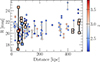 |
Fig. 1. Magnitude and projected distance of the quasar pairs presented in this work (squares) and found in catalogs (circles). The points are color-coded by redshift. |
The sample is selected from the SDSS DR12 quasar catalog (Pâris et al. 2017) and AGN searches at high-z (e.g., Bielby et al. 2013) as described in Arrigoni Battaia et al. (2019b), Cai et al. (2018), and Herwig et al. (2024). Specifically, quasars are required to be within 1′ (or approximately 500 kpc at the median redshift) and Δz ≤ 0.03 (or roughly Δv < 2000 km s−1) of each other to achieve a high likelihood of physical association and therefore a local AGN overdensity. The observed sample spans a redshift range between z = 2.45 and z = 3.83 with a median redshift of 3.13. We visualize magnitude, projected pair separation, and redshift of our sample compared to pairs found in the Million Quasars (Milliquas) v8 catalog (Flesch 2023) and the aforementioned catalogs between z = 2 and z = 4 and on the full sky. While the magnitudes of our sample are typical, the observed pairs do not cover intermediate projected separations between 150 kpc and 400 kpc.
For seven pairs or pair members, rest-frame ultraviolet integral-field unit observations are available probing Lyα emission on scales of the circumgalactic medium within a few hundred kiloparsecs around the quasars using the Multi-Unit Spectroscopic Explorer on the Very Large Telescope (IDs 1 to 6, Herwig et al. 2024) or the Palomar and Keck Cosmic Web Imager (ELAN0101, Cai et al. 2018). The SCUBA-2 observations were performed with an exposure time of about 30 minutes per scan between May 24, 2022, and January 11, 2023, under very good (τ < 0.05, program ID M22BP025) and good (τ < 0.08, program ID M22AP049) weather conditions using a Daisy scanning pattern centered on one of the quasars in the pair and covering a field of view (FoV) of around 13.7′ in diameter. At the median redshift of the sample, this corresponds to a diameter of 6.4 physical Mpc and is comparable to the expected size of protoclusters at these redshifts (Chiang et al. 2017). We obtained observations of the 450 μm band with an effective beam FWHM of 9.8″ and of the 850 μm band with an effective beam FWHM of 14.6″.
We performed the data reduction following the methods described in Chen et al. (2013) and employed in Nowotka et al. (2022) and Arrigoni Battaia et al. (2023), utilizing the Dynamic Iterative Map Maker (DIMM) from the SMURF package within the STARLINK software (Jenness et al. 2011; Chapin et al. 2013). We processed each scan using the standard configuration file, dimmconfig_blank_field.lis. The reduced scans were then combined into final maps using the MOSAIC_JCMT_IMAGES recipe in PICARD, the Pipeline for Combining and Analyzing Reduced Data (Jenness et al. 2008). To enhance point source detectability, we applied a standard matched filter to the final maps using the PICARD recipe SCUBA2_MATCHED_FILTER. Finally, we employed the latest flux conversion factors of 472 Jy beam−1 pW−1 for the 450 μm map and 495 Jy beam−1 pW−1 at 850 μm (Dempsey et al. 2013; Mairs et al. 2021), which include the correction of a flux decrease introduced by the matched filter technique. In the 850 μm maps of ID2, two out of three exposures show interference patterns and we excluded them from the combination and analysis.
This procedure results in one signal map and one noise map per observed field and wavelength band. Excluding ID2, the central noise in the final maps spans from 6.54 mJy beam−1 to 13.94 mJy beam−1 at 450 μm and from 0.79 mJy beam−1 to 1.24 mJy beam−1 at 850 μm. The noise increases significantly toward the edges of the maps and thus we only considered pixels below 2.5 times the central noise for the following analysis. The region satisfying this condition is called the effective area Aeff.
To obtain true noise maps, we employed the jackknife technique by dividing the exposures for each band and field into two maps containing roughly half of the exposure time each, and subtracting these maps from each other. We rescaled the two maps by the factor  to match the exposure times t1 and t2 in the two maps. Because of the strong weather dependence of the data sensitivity at 450 μm, we ensured that the weather conditions in the exposures of each image are roughly equal. In this way, any true source irrespective of its significance will be removed from the jackknife map and only noise features remain. As only one exposure at 850 μm for the field of quasar pair 2 is available, we cannot construct jackknife maps for the object and exclude it from any further analysis requiring true noise maps. For quasar pair 4, only three exposures are available and we cannot divide them according to weather conditions, leading to an increased central noise of 14.8 mJy beam−1 at 450 μm. The central noise in the rest of the jackknife maps is consistent with the central value in the noise maps, deviating only by a maximum of 2.9% at 850 μm, with values between 0.78 mJy beam−1 and 1.28 mJy beam−1, and up to 6.8% at 450 μm, spanning from 6.50 mJy beam−1 to 12.1 mJy beam−1.
3. Source extraction
We extracted sources that lie fully within the respective effective area by identifying the highest S/N peak, writing relevant information to the source catalog and removing this source from the map by subtracting a scaled empirical point spread function (PSF) taken from Chen et al. (2013) as galaxies are not resolved at the low spatial resolution of the data. We repeated this process until the highest S/N value fell below three. Sources consistent (i.e., within 6″) with any quasar positions in these initial source catalogs and their counterpart source detection in the other band are summarized in Table A.1 of Appendix A. Out of the sample of 18 quasars, eight are detected above 3σ, consistent with the quasar detection rate of Arrigoni Battaia et al. (2023), who detect nine out of twenty quasars with the same observing strategy.
To increase the reliability of source detection, we cleaned the catalogs by removing any source below 4σ that is not detected in both bands above 3σ. Further, we identified all sources from the catalog at 850 μm that are detected in both bands, but whose deboosted fluxes within errors do not fit the ratio expected from an SMG SED (da Cunha et al. 2015) at the redshift of the quasar pair and ±9000 km s−1 away from it. These are likely low-redshift interlopers, multiple blended sources or SMGs with significant contribution from a dust-obscured AGN, leading to an atypical SED. In total, we identified 26 interloper or non-SMG candidates, with a median value of one per field, and summarized them in Table B.1 (available only in electronic form).
In this way, we obtained two source catalogs for each quasar pair field with more detections at 850 μm (median 20 excluding ID2) than at 450 μm (median three) due to the lower noise level in the first band. In total, we identified 170 SMG candidates in the 850 μm band (Fig. 2, Tables C.1 – C.9, available only in electronic form).
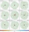 |
Fig. 2. S/N maps at 850 μm. The position of the brighter (fainter) quasar is indicated by a black (brown) star. Identified catalog SMGs are marked by black circles with the same size as the effective beam FWHM of 14.6″. The gray dashed line indicates the edge of the effective area (2.5 × the central rms). Sources inconsistent with the expected SMG SED at the quasar redshift are marked with gray rectangles. |
3.1. Reliability
A commonly adopted method for determining the reliability of source extraction is the inversion of the signal map and extraction of a source catalog from the inverted map. This method relies on the assumption that noise peaks have the same absolute value as noise troughs (i.e., peaks in the inverted map). However, this is not the case for maps processed with the matched filter approach as it introduces very negative values around the PSFs of the brightest sources. Thus, in median, we detected eight spurious sources in the inverted 850 μm maps (excluding ID2), which show more numerous and more significant source detections, but only a median of one spurious source at 450 μm.
We therefore determined the reliability of our source detection using the jackknife maps instead, as done in Arrigoni Battaia et al. (2023). For this, we extracted sources from the jackknife map following the same procedure as detailed in Sect. 3. Since spurious sources do not have counterparts, we only extracted data peaks above 4σ. We found a median number of 1.5 spurious sources at 450 μm and 0.5 spurious sources at 850 μm, in agreement with or lower than previous works (Arrigoni Battaia et al. 2018a, 2023). As a similar number of false detections is expected to occur in the source catalogs at 850 μm, we obtain a reliability of 97.6%.
3.2. Completeness
We determined the flux at which the source extraction can be considered complete by injecting sources into the effective area of the jackknife maps using the same PSF as during source extraction and attempting to recover them using the same algorithm as in Section 3. In the map of the 850 μm band, we injected 10 000 sources each for fluxes between 0.1 mJy and 30.1 mJy in 0.5 mJy steps, while at 450 μm, we used fluxes between 0.1 mJy and 80.1 mJy in 1 mJy steps. Fig. 3 displays the resulting completeness percentage per flux.
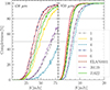 |
Fig. 3. Completeness percentage of the source extraction as a function of injected source flux in the 450 μm band (left) and the 850 μm band (right). |
The completeness is mainly affected by the weather conditions during the observations and the number of scans used in the combined map and can stay particularly low at 450 μm (< 50% in field 4 for any injected source flux).
4. Differential number counts
We aim to characterize the SMG overdensity around quasar pairs in comparison to the field and thus require knowledge of the underlying source model in the observed 850 μm maps centered on quasar pairs, which we reconstructed from differential number counts. We followed the methods described in Chen et al. (2013).
As a first step, we determined the S/N at which the number of pixels in the data map is significantly larger than in the jackknife map (i.e., ≥3×), meaning that those pixels are mostly dominated by sources. On average, this condition is fulfilled at a S/N of 2.9, ranging between 2.5 and 3.3. We used these values as a new detection threshold to extract sources from the data maps. Naturally, the lower S/N requirement leads to a lower reliability of source extraction, as quantified by extracting all spurious sources down to the same S/N threshold in the jackknife maps (analogously to Sect. 3.1). However, as we are only interested in the raw number counts and fluxes instead of the position of sources, we can use this number to correct the raw number counts for reliability. For that, we divided detections into equally spaced logarithmic flux bins and normalized the number counts by bin width and detectable area, defined as the area of the map in which the noise is low enough that a source of the given flux would reach the S/N threshold. After processing the number counts from the jackknife maps in the same way, we subtract these spurious sources from the data number counts.
The resulting data points are affected by multiple observational biases such as incompleteness, flux boosting, and source blending, that typically increase the observed differential number counts for a given flux bin and thus have to be taken into account to obtain the underlying source model to evaluate the galaxy overdensity. To reconstruct it by finding a model that reproduces the observed raw number counts, we used Monte Carlo simulations following the exact procedure of Nowotka et al. (2022) that we briefly summarize below. For easier comparison with blank field models such as Geach et al. (2017), we parameterized the model using the same Schechter function as in that work,
with the normalization N0 (in deg−2) and the characteristic flux S0 (in mJy), which is fixed to a value of 2.5 mJy to avoid the degeneracy between N0 and S0. To get a set of initial parameters, we fit the raw number counts in the quasar pair fields with the Schechter function and created 100 different mock maps by injecting sources sampled from the model down to 1 mJy (as done in previous work; e.g., Nowotka et al. 2022) at random positions of the corresponding jackknife map. From these realizations, we obtained average number counts and used them to adjust the raw number counts by multiplying with the ratio of raw counts to mean recovered counts. The simulation then repeats from the Schechter function fitting now using the adjusted points and only stops once the mean recovered counts are within 1σ of the raw counts in three consecutive loops (green versus black data points in Fig. 4). For some fields (e.g., ID 3), the highest flux bin had to be excluded from the fit to achieve convergence due to small number statistics. The parameters of the converged Schechter functions are summarized in Table 2.
Parameters of the Schechter functions reproducing the observed source counts, galaxy overdensities calculated from the models, and angle direction of the overdensities.
We further verified that the source model found through Monte Carlo simulations properly reproduces the observed data including all observational biases by creating 500 mock maps per field and comparing the recovered source count with the observed counts. Finally, we created 500 mock maps of the field by injecting sources according to the field model found by Geach et al. (2017) (fiducial model) with N0 = 7180 ± 1220 deg−2, S0 = 2.5 ± 0.4 mJy, and γ = 1.5 ± 0.4. In that work, the blank field was derived from almost 3000 submillimeter source detections in 850 μm SCUBA-2 maps covering an area of roughly 5 deg2. This test instructs us on whether the blank field source model is consistent with our observed differential number counts or not. The differential number counts and confidence intervals obtained from the 500 realizations as well as the underlying source models are displayed in Fig. 4. Additionally, we used the 500 simulated maps of the underlying source model per field to quantify the flux boosting and positional uncertainty Δ(α, δ) of the source extraction at 850 μm by comparing the position and flux of the injected and recovered sources. Since we do not recover an underlying source model at 450 μm, we instead injected sources according to the model found by Casey et al. (2013) to obtain the boosting factor and positional uncertainty.
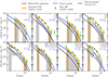 |
Fig. 4. Differential number counts at 850 μm in the data (green points), underlying source model of the quasar pair fields (blue), and 1σ spread of the differential number counts from 500 realizations of the source model (yellow shaded area). For comparison, we show the fiducial field model (black dashed) with its 1σ spread in 500 realizations (gray shaded area). We report the overdensity factor δcumul for each field in the panels. |
5. Results
5.1. Galaxy overdensity factors
From the reconstructed underlying source models (Fig. 4), the overabundance of SMGs in the field of quasar pairs in comparison to the fiducial model (Geach et al. 2017) is evident. To quantify the degree of this effect, we calculated galaxy overdensity factors based on the model normalization (δscaled) and the cumulative differential number counts (δcumul) as previously done in Nowotka et al. (2022).
Specifically, to obtain δscaled, we scaled the observed differential number counts by the ratio between the underlying model and the mean recovered number counts to correct for observational biases and fitted the field model from Geach et al. (2017) to the resulting points, using the symmetrized error bars as weights and leaving the normalization factor N0 free to vary. The ratio between normalization factors of the quasar pair fields and the fiducial model is then δscaled. The obtained values have a weighted average of 2.7 ± 0.1 and are compiled in Table 2. This method is particularly successful if the slopes of the Schechter functions are similar to the fiducial model (e.g., ID 6 and ID ELAN0101), but does not capture the full picture for fields with values of γ very different from γ = 1.5. Thus, we additionally calculated the cumulative overdensities δcumul by integrating the source models between the minimum and maximum flux of detected sources and determining the ratio to the fiducial model integrated in the same range. To obtain a robust value and the typical error range, we randomly vary all free parameters of the two models within their 1σ error 50 000 times. The values for δcumul and their errors are then obtained from the median, 16th, and 84th percentile of the resulting distribution and also listed in Table 2. By symmetrizing the error, we obtained the weighted average of 3.4 ± 0.3 for the overdensity factor determined in this way. The implication of the calculated overdensity factors are discussed in Sect. 6.1.
5.2. Star formation rates and molecular gas masses
Because the dust temperature and therefore the emission at submillimeter wavelengths is driven by the obscured star formation, we can calculate the SFR and dust mass Md for each source from its 850 μm flux. We use the relations found by Dudzevičiūtė et al. (2020) based on ALMA data and UV-to-radio SED fitting of 707 SMGs, selected from the SCUBA-2 Cosmology Legacy Survey (Geach et al. 2017), log(SFR/(M⊙ yr−1)) = (0.42 ± 0.06)×log(S870/mJy)+(2.19 ± 0.03) and log(Md/(M⊙)) = (1.20 ± 0.03)×log(S870/mJy)+(8.16 ± 0.02). We calculated the cumulative SFRs and molecular gas masses Mgas, assuming a gas-to-dust ratio of 63 (Birkin et al. 2021), of all SMG candidates and quasar detections with respect to the coordinate in the middle between the quasar pair for each field and compared the SFRs to literature protoclusters (Wang et al. 2025 and references therein), the cumulative SFRs of the ten simulated protocluster regions in FOREVER22 (Yajima et al. 2022) at z = 3, and the 32 most massive halos at the respective redshift from the Magneticum Pathfinder simulation (Remus et al. 2023; Dolag et al. 2025). The SFRs from simulations include all types of star-forming galaxies and are not limited to massive, dusty galaxies equivalent to SMGs or flux-limited in agreement with the observations. To compare to the gas mass in the 32 Magneticum halos, we assumed a molecular-to-atomic gas ratio between 10%, corresponding to the lowest estimates for small galaxies (Saintonge et al. 2011; Catinella et al. 2018), and 70%, found in highly star-forming, massive galaxies (Saintonge et al. 2016).
FOREVER22 is a set of zoom-in hydrodynamical simulations of protocluster regions selected at z = 2 from the parent N-body box of 714 cMpc per side and each simulated in a box size of (28.6 cMpc)3 until zend = 2. At z = 0, the selected halos span masses between 5.2 × 10¹⁴ M⊙ h−1 and 1.4 × 10¹⁵ M⊙ h−1. The initial gas particle mass is set to 2.9 × 10⁶ M⊙ h−1 and the gravitational softening length is 2 ckpc h−1. Magneticum is a set of hydrodynamic simulations of cosmological boxes, including Box2b of 640 Mpc h−1 per side from which the displayed halos are selected. It is simulated to z = 0.2 with a gas particle mass of 1.4 × 10⁸ M⊙ h−1 and a gravitational softening length of 3.75 kpc h−1. The virialized halo masses of the displayed protocluster regions at z = 2.79 span masses log(M/M⊙h−1) = 13.6 − 14.1 (log(M/M⊙h−1) = 13.4 − 14.3 for all four redshifts). Although not all the selected regions will collapse into galaxy clusters by z = 0, the likelihood increases with decreasing redshift and almost all halos selected at z = 2 end as one in the last simulation snapshot (Remus et al. 2023).
The resulting cumulative SFRs are shown in Fig. 5, and the cumulative Mgas are displayed in Fig. 6. As both distributions depend not only on the detected fluxes of the sources, but also on the raw cumulative source count, we show the latter in Appendix D for comparison. Because the calculations rely on source detections, our observational values are heavily influenced by the data quality as the completeness of the source detection decreases under worse observing conditions and shorter exposure time, and we thus attempted to correct for these effects when converting SFRs to SFR densities in two different ways. Firstly, we calculated SFRDint by integrating the obtained underlying source model (Table 2) multiplied with the SFR relation in the range S850 = (1 − 20) mJy and weighting the result by the volume of a sphere with a projected area of Aeff (Table 1). The 16th, 50th and 84th percentile range give SFRD , and the weighted average is SFRDint = 1700 ± 100. Given the completeness curve and assuming a uniform source model throughout the structure, we would expect to detect only up to 12% of the SFR derived in this way.
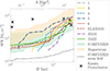 |
Fig. 5. Cumulative SFR of the quasar pair fields compared to the ten protocluster zoom-in simulations of FOREVER22 at z = 3 (Yajima et al. 2022), the 32 most massive halos from Magneticum at z = 2.79 (Remus et al. 2023; Dolag et al. 2025), and known protoclusters from the literature (Wang et al. 2025 and references therein). The dotted line shows the cumulative SFR of the mean blank field in FOREVER22 (Yajima et al. 2022). |
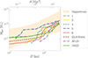 |
Fig. 6. Cumulative molecular gas mass Mgas of the quasar pair fields compared to the molecular gas mass in the 32 most massive halos in Magneticum at z = 2.79 (Remus et al. 2023; Dolag et al. 2025), estimated from the star-forming gas. |
We then calculated SFRDcen by only summing up source detections, including SMG candidates and quasar detections, within the central 1 Mpc and weighting them by the completeness within this smaller aperture and the volume of a sphere with 1 Mpc radius. The median value is SFRD , while the weighted average is SFRDcen = 204 ± 97, dominated by fields with few central detections, and therefore low total error.
A flux-SFR conversion relation based on ALMA data can lead to further uncertainties if applied to SCUBA-2 data, due to the difference in beam size. We thus calculated the SFRs using the relation reported in Cowie et al. (2017) based on photometrically selected SMGs and find higher values for every field with an average increase of 45% in SFRDint and 75% in SFRDcen. However, we opt to report the more conservative values derived from redshift-confirmed SMGs, and compile the results in Table 2.
For comparison, we also calculated SFRDint and SFRDcen for the source models of single quasar fields (median values with 16th and 84th percentile ranges of SFRD and SFRD
 , weighted average SFRDint = 1700 ± 100 and SFRDcen = 400 ± 100) and ELAN fields reported in Arrigoni Battaia et al. (2023), and calculate SFRDint and SFRDcen for PCR0 in FOREVER22 and the most massive halo of the Magneticum Box2b by summing up sources within 3 Mpc (i.e., the typical radius obtained from Aeff in the quasar pair fields) and 1 Mpc respectively. The results are shown in Fig. 7. We also compare to the redshift evolution of the cosmic mean SFRD (MD14; Madau & Dickinson 2014), the mean field SFRD in Box2b of Magneticum (Dolag et al. 2025), and predictions of the mean SFRD in protoclusters from the Manhatten suite of 100 zoom-in simulations of protocluster regions with M > 1014 M⊙ selected at z = 2 as the most massive halos from an N-body box with a side length of 1.5 cGpc (Rennehan 2024). The zoom-in areas include 9×Rvir at a gas particle mass resolution of roughly 3.5 × 10⁷ M⊙ and an adaptive gravitational softening length, but a minimum value of 0.73 ckpc. Overall, Figures 5 to 7 show that although our candidate SMGs represent only a fraction of the total SFR and cold gas mass in simulated protocluster structures because of the exclusion of less obscured star-forming galaxies, our measurements are in agreement with model predictions when considering potential incompleteness of the observations. We further discuss the derived values for SFR and SFRDs from our observations and their connection to simulation values in Sect. 6.1.
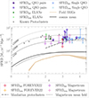 |
Fig. 7. SFRD in the central 1 Mpc (SFRDcen) and from the source model of the full field (SFRDint) for quasar pairs, ELANe (Nowotka et al. 2022; Arrigoni Battaia et al. 2023), and single quasars (Arrigoni Battaia et al. 2023), compared to values reported for known protoclusters (Clements et al. 2014; Dannerbauer et al. 2014; Kato et al. 2016) and simulation predictions from FOREVER22 (PCR0; Yajima et al. 2022) and Magneticum Box2b (the most massive halo; Remus et al. 2023), both integrated within the central 1 Mpc (SFRDcen) and 3 Mpc (SFRDint). The solid black line shows the mean cosmic SFRD (Madau & Dickinson 2014); the solid gray lines are the mean cosmic SFRD scaled up by a factor of 100, 1000, and 10 000, respectively; the beige line shows the SFRD for blank field SMGs (Dudzevičiūtė et al. 2020); the dash-dotted line shows the simulation prediction for SFRD within protoclusters by Rennehan (2024); and the dotted line is the SFRD in the Magneticum mean field (Dolag et al. 2025). |
5.3. Direction of overdensity
We determined the preferred direction of the galaxy overdensity in each field using two different methods following Arrigoni Battaia et al. (2023). If massive galaxies such as SMGs are tracers of filaments connecting to the quasar in the center, this direction would be equivalent to the projection of a cosmic web filament. Using the coordinate in the middle between the quasars as a reference point, we first calculated the angle αRMS (measured from East to North) that minimizes the rms distance of detected sources weighted by the completeness. For robust results, we performed the calculation in 50 000 randomly drawn subsamples encompassing 90% of the sources with replacement, smoothed the obtained angle distribution using a Gaussian kernel density estimate, and defined the peak as αRMS. We obtained errors from the 16th and 84th percentile. Second, we determined the angle αinertia by computing the 2D inertia tensor from the source positions weighted by completeness and obtaining the eigenvector that minimizes the eigenvalue (Zeballos et al. 2018). Equivalently to the other method, we used the peak value and 16th and 84th percentile of the angle distribution from 50 000 90% subsamples to get αinertia and the corresponding errors. In all cases, αRMS and αinertia are consistent with each other within error bars. The values are compiled in Table 2 and the preferred SMG directions and source weights are displayed in Fig. 8, together with the line connecting the two quasars and the direction of the semimajor axis of the Lyα nebula, if available from Herwig et al. (2024). For ELAN0101, we obtained the nebula semimajor axis analogously to the calculation in Herwig et al. (2024) from Figure 1 (upper right panel) in Cai et al. (2018). We note that choosing one of the quasars as reference point instead does not significantly impact the obtained angles. Specifically, αRMS deviates by less than 6°, while αinertia can differ by up to 12°. In Appendix E, we show the success in recovering the angle direction of simulated SMG distributions within filaments of different widths. The calculated angles and related findings are discussed in Sect. 6.2.
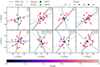 |
Fig. 8. Direction of the overdensity calculated from the eigenvalue and the minimized rms, as well as the line connecting the quasar pair and the semimajor axis of the nebula, if available. All catalog sources of the fields are plotted; the size and color of the points indicate the weight according to catalog completeness at the flux of the SMG (i.e., within one field; larger and brighter points correspond to higher fluxes). |
6. Discussion
6.1. Do quasar pairs trace protocluster environments?
Contrary to previous studies of single AGN fields (Rigby et al. 2014; Jones et al. 2017; Arrigoni Battaia et al. 2023), we find an increased density of SMGs in all objects of our sample of quasar pair fields and observe a cumulative SFR and SFRD roughly in agreement with known protoclusters from the literature and simulations and, compared to the field, increased by a factor of 100 to 100 000. If the majority of detected sources are truly associated with the quasar pairs, these findings strongly support the hypothesis that quasar pairs indeed trace protocluster environments. While we attempted to exclude interlopers using the 450 μm band, fainter interloping galaxies undetected in this band can still contaminate the sample, and in particular, the typical SED of an SMG is expected to peak within the SCUBA-2 bands for lower-z sources. Therefore, follow-up observations are necessary for definitive redshift confirmation of the SMG candidates, though the comparatively high overdensities support physical association with the quasar pairs, and the distribution of SMGs peaks at z = 2 − 3. On the other hand, SCUBA-2 observations using the daisy scan pattern lead to stark differences in the sensitivity throughout the field as the noise quickly increases toward the edges of the image. Thus, employing this observational strategy, we would likely miss important parts of the galaxy population in our SMG candidate catalogs if the quasar pair is offset from the center of a forming galaxy protocluster, and imaging with uniform sensitivity throughout the likely protocluster extent of roughly 20 cMpc would alleviate this problem.
An offset between the reference point of our observations and the true protocluster center could potentially also explain why most simulated protoclusters show higher cumulative SFRs in the center compared to the quasar pair fields observed here (Fig. 5), though quasar pairs still significantly exceed the mean field expectation from FOREVER22 and lie within the range of SFR for its ten protocluster zoom-ins for most radii, including the protocluster centers. Alternatively, the central SFR might not be dust obscured in all quasar pair fields and thus would not appear at submillimeter wavelengths, while the SFRs obtained for simulated protoclusters include all types of star-forming galaxies and are therefore expected to be shifted toward higher values. On the other hand, most cosmological simulations are known to not reproduce the extremely bursty SFR observed in SMGs well (Bassini et al. 2020; Lim et al. 2021; Remus et al. 2023), leading to a potential suppression of the cumulative SFR. At the largest studied radii, the cumulative SFR of the quasar pair fields exceeds the predictions from the FOREVER22 simulations, but most data points stay below the cumulative SFRs in Magneticum protoclusters, with the exception of quasar pair 5, the field hosting a candidate quadruple AGN in the center (Herwig et al. 2025), which fits the radial profile of the Magneticum predictions well. On the other hand, the cumulative molecular gas masses Mgas of the observed quasar pairs are in good agreement with the Magneticum predictions (Fig. 6), though the uncertainty in molecular-to-ionized gas ratio and gas-to dust-ratio are large. The central cumulative SFR around quasar pairs is also lower than in other known protoclusters, although all but one are indeed dominated by central SFR within 1 Mpc from the quasar pair (Fig. 7) and the median values and weighted averages of SFRDcen and SFRDint are consistent between quasar pairs and single quasars within error bars. This is in agreement with ELANe, while single quasar fields are instead dominated by extended SFR in more than a third of the fields reported in Arrigoni Battaia et al. (2023). Large cool gas reservoirs are expected to be a necessary requirement to drive both ELAN and AGN activity in multiple quasars, and could feasibly feed an abundance of SFR in the central region of a protocluster simultaneously, explaining the excess of SFRDcen compared to SFRDint. The SFRD for spectroscopically confirmed blank field SMGs (Dudzevičiūtė et al. 2020) compared to the cosmic mean SFRD (Madau & Dickinson 2014) shown in Fig. 7 further highlights the contribution from non-SMGs to the SFRD and therefore likely the SFR in protocluster regions and the necessity for multiwavelength observations of the quasar pair fields presented in this work for a comprehensive view of the potential protocluster regions and a better comparison to simulations. The central SFRD in the Magenticum and FOREVER22 simulations are of the same order of magnitude as observed protoclusters and protocluster candidates, while the SFRD integrated over larger areas tend toward lower values, especially for the FOREVER22 zoom-ins and as already seen in Fig. 5. Additionally, Magneticum reproduces the mean field SFRD well. Predictions for the SFRD within all 100 protoclusters of the Manhattan suite of simulations fit observational data points above z ∼ 3, but show a steeper decline toward low redshifts. This could be a consequence of their selection based on mass at z = 2, which might require a starburst peak at higher redshifts to build up sufficient mass.
The presented average SMG overdensity of δcumul = 3.4 ± 0.3 in quasar pair fields significantly exceeds the average value of δcumul = 2.5 ± 0.2 found around single quasars with a similar approach as employed here (Arrigoni Battaia et al. 2023), but is consistent with previously reported values for fields with multiple known quasars, δcumul = 3.6 ± 0.6 (Nowotka et al. 2022) and δcumul = 3.4 ± 0.4 (Arrigoni Battaia et al. 2023). While half of our sample has higher overdensity factors than the peak value of δcumul = 3.9 reported in both works, this is possibly a statistical effect. The two studies targeted the environment of quasars associated with an ELAN and concluded that these extreme Lyα nebulae are suitable tracers of galaxy overdensities. In contrast to that, we find the lowest overdensity factor in the only field of our sample with a known ELAN (ELAN0101) with δcumul = 2.6 ± 0.9. Instead, our findings suggest that the galaxy overdensities are causally connected to AGN overdensities, which are typically needed to power exceptionally far extended Lyα emission and are thus present in all ELAN fields. As such, we find the highest overdensity factor of δcumul = 4.6 ± 1.7 around the quadruple AGN candidate (ID5), further highlighting this system as the most interesting field for follow-up studies and the most likely protocluster region of our sample. In most fields (six out of eight), at least one quasar of the pair is detected above 3σ at 850 μm, but the quadruple AGN candidate is associated with the brightest emission from any quasars in both bands. It also stands out as the only system of the sample with a radio-loud quasar detected in VLA FIRST (Becker et al. 1994), though the radio emission location is consistent with the position of the brighter quasar and the two AGN candidates accompanying it (Herwig et al. 2025).
6.2. Comparison of different methods to infer filament direction
We attempted to infer the direction of cosmic web filaments in three different ways for most fields: the preferred alignment direction of detected SMG candidates (αRMS, αinertia), the line connecting the two quasars as they are likely connected by a filament due to their proximity and large halo mass, and the semimajor axis of the Lyα nebulae, if available from Herwig et al. (2024), as the extended emission might trace cool gas accreted onto the circumgalactic medium from filaments connecting to the halo (Costa et al. 2022). While Herwig et al. (2024) found alignment of the latter two values for all Lyα nebulae extending for more than 70 kpc from the brighter quasar (ID1, ID4, ID6), these angles do not coincide with the preferred direction of SMGs. In fact, in most cases and irrespective of projected quasar pair separation, pair direction and Lyα emission direction are almost perpendicular to the SMG direction (ID1, ID4, ID6 for αRMS, ELAN0101, J0119, J1622). Only two fields (ID3 and ID5) show signs of alignment of the Mpc-scale galaxy distribution and the kiloparsec-scale quasar pairs or their extended Lyα emission. This finding is in agreement with Arrigoni Battaia et al. (2023), who found alignment between SMGs and Lyα nebulae for single quasar fields, but average offset angles of  and
and  for ELAN fields (i.e., fields with multiple quasars). To further highlight this point, we show the distribution of angle offsets between SMG distribution and Lyα nebula, restricted to angles between 0° and 90°, for different known quasar number per field in Fig. 9. While the median values with 16th and 84th percentile error (
 degrees and
  degrees for single quasar fields and multiple quasar fields respectively) are consistent within errors of each other, the most dominant bin for single quasar fields spans from 0 degree to 10 degree, while most multiple-AGN fields can be found at an offset angle between 70 and 80 degrees.
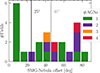 |
Fig. 9. Histogram of the angle difference between semimajor axis of the nebula and direction of the megaparsec-scale SMG distribution αRMS, color-coded by the number of quasars in the center of the field. The angles are compiled from Arrigoni Battaia et al. (2023), Herwig et al. (2024), and Table 2, and are restricted to the range [0° ,90°). The median angle offset of 25° (46°) for single (multiple) quasar fields is marked by the vertical black (gray) line. |
A possible cause for the misalignment could be the increased importance of galaxy interactions for the Lyα nebula morphology in the dense regions of quasar pairs. In this picture, the angles measured from quasars and extended Lyα emission might trace small-scale dense gas filaments shaped by a potential ongoing galaxy merger, while SMGs trace large-scale filaments which would only sometimes coincide in projection due to a random occurrence. Further, the connectivity of halos to the cosmic web increases with increasing halo mass (Galárraga-Espinosa et al. 2024). In other words, more cosmic web filaments are expected to be linked to a halo the higher its mass. If two quasars are physically associated, their combined halo mass would increase the likelihood of a complicated structure of gas filaments in their direct environment, and their directions might not be simply described by a straight line determined from the surrounding galaxy population. Further complicating the geometry of filaments within protocluster regions, the most massive SMGs have similarly high halo masses as quasars and therefore likely reside in nodes of the cosmic web themselves. However, the majority of the population consists of less massive galaxies that should preferentially lie along the spines of filaments. Another potential cause for a preferential alignment direction of the SMGs is radiative feedback from quasars, which may biconically suppress star formation in their proximity zone. While previous studies suggest that this feedback primarily affects low-mass halos (e.g., Bosman et al. 2020; Champagne et al. 2025), the presence of two bright quasars could boost the radiation sufficiently to quench star formation in more massive galaxies close to the quasars in the direction of the ionization cone, thus leading to an alignment of SMGs perpendicular to it. We defer further tests of this hypothesis, such as studying the positions of Lyα emitters around the quasar pairs, to future work.
7. Summary and conclusions
Using JCMT/SCUBA-2 850 μm imaging covering an area of 106 arcmin2 on average (or 23.1 Mpc2 at the median z = 3.13), we searched for submillimeter sources around nine quasar pairs at z = 2.45 − 3.83. Our main findings are as follows:
-
We identified 170 SMG candidates at 4σ significance in the 850 μm band or at 3σ significance in both the 850 μm and 450 μm band, 26 interloper or non-SMG candidates, and eight detections >3σ for quasars.
-
All objects targeted in this work are surrounded by SMG overdensities when compared to blank fields, with an average overdensity factor of δcumul = 3.4 ± 0.3, confirming that within our sample, physically associated quasar pairs are reliable tracers of galaxy overdensities. δcumul is similar to ELAN fields, and significantly higher than around single quasars.
-
The cumulative SFR and SFRDs are consistent with theoretical predictions for protoclusters, known protoclusters, and single quasar fields, although SFR around quasar pairs tends to be more centrally peaked when compared to single quasars.
-
We do not find alignment between the direction of the SMG overdensity and the quasar pair direction or the semimajor axis of extended Lyα emission associated with the circumgalactic medium of the quasar pairs, indicating that SMGs might trace different, larger-scale filaments than the other metrics.
This work showcases the utility of quasar pairs in pinpointing dense megaparsec-scale environments. The overdensity factors and SFRDs identify the studied fields as likely sites of protocluster formation. However, spectroscopic follow-up studies of all SMG candidates proposed in this work are necessary to confirm the density and geometry of the structures surrounding quasar pairs. To get a complete view of the galaxy population around quasar pairs and test the filament direction inferred from the SMG distribution against other methods, multiwavelength observations identifying smaller star-forming galaxies such as Lyα emitters (e.g., García-Vergara et al. 2019) or Lyman break galaxies (Steidel et al. 2003) are necessary.
Data availability
Tables B.1 and C.1 to C.9 are available at the CDS via https://cdsarc.cds.unistra.fr/viz-bin/cat/J/A+A/703/A17
Acknowledgments
We thank the anonymous referee for their evaluation of this work that helped improve the manuscript and Guinevere Kauffmann for providing useful comments to an earlier version of this work. This work made use of data taken under the Program IDs M22AP049 and M22BP025. These observations were obtained by the James Clerk Maxwell Telescope, operated by the East Asian Observatory on behalf of The National Astronomical Observatory of Japan; Academia Sinica Institute of Astronomy and Astrophysics; the Korea Astronomy and Space Science Institute; the National Astronomical Research Institute of Thailand; Center for Astronomical Mega-Science (as well as the National Key R&D Program of China with No. 2017YFA0402700). Additional funding support is provided by the Science and Technology Facilities Council of the United Kingdom and participating universities and organizations in the United Kingdom and Canada. Additional funds for the construction of SCUBA-2 were provided by the Canada Foundation for Innovation. The authors wish to recognize and acknowledge the very significant cultural role and reverence that the summit of Maunakea has always had within the indigenous Hawaiian community. We are most fortunate to have the opportunity to conduct observations from this mountain. Computations were performed on the FREYA cluster hosted by The Max Planck Computing and Data Facility (MPCDF) in Garching, Germany. We acknowledge the support provided by the MPCDF helpdesk. This work has made use of the Python libraries matplotlib (Hunter 2007), numpy (van der Walt et al. 2011), astropy (Astropy Collaboration 2013, 2018, 2022), and scipy (Virtanen et al. 2020). C.-C.C. acknowledges support from the National Science and Technology Council of Taiwan (111-2112-M-001-045-MY3), as well as Academia Sinica through the Career Development Award (AS-CDA-112-M02). A.O.’s contribution to this work was made possible by funding from the Carl Zeiss Stiftung. H.Y. acknowledges support by MEXT/JSPS KAKENHI Grant Number 21H04489 and JST FOREST Program, Grant Number JP-MJFR202Z. The Magneticum Pathfinder simulations were performed at the Leibniz-Rechenzentrum with CPU time assigned to the Project pr83li. This work was supported by the Deutsche Forschungsgemeinschaft (DFG, German Research Foundation) under Germany’s Excellence Strategy EXC-2094 – 390783311. We are especially grateful for the support by M. Petkova through the Computational Center for Particle and Astrophysics (C2PAP).
References
- Arrigoni Battaia, F., Chen, C.-C., Fumagalli, M., et al. 2018a, A&A, 620, A202 [NASA ADS] [CrossRef] [EDP Sciences] [Google Scholar]
- Arrigoni Battaia, F., Prochaska, J. X., Hennawi, J. F., et al. 2018b, MNRAS, 473, 3907 [NASA ADS] [CrossRef] [Google Scholar]
- Arrigoni Battaia, F., Hennawi, J. F., Prochaska, J. X., et al. 2019a, MNRAS, 482, 3162 [NASA ADS] [CrossRef] [Google Scholar]
- Arrigoni Battaia, F., Obreja, A., Prochaska, J. X., et al. 2019b, A&A, 631, A18 [EDP Sciences] [Google Scholar]
- Arrigoni Battaia, F., Obreja, A., Chen, C. C., et al. 2023, A&A, 676, A51 [NASA ADS] [CrossRef] [EDP Sciences] [Google Scholar]
- Astropy Collaboration (Robitaille, T. P., et al.) 2013, A&A, 558, A33 [NASA ADS] [CrossRef] [EDP Sciences] [Google Scholar]
- Astropy Collaboration (Price-Whelan, A. M., et al.) 2018, AJ, 156, 123 [Google Scholar]
- Astropy Collaboration (Price-Whelan, A. M., et al.) 2022, ApJ, 935, 167 [NASA ADS] [CrossRef] [Google Scholar]
- Barger, A. J., Cowie, L. L., Sanders, D. B., et al. 1998, Nature, 394, 248 [Google Scholar]
- Barger, A. J., Cowie, L. L., & Richards, E. A. 2000, AJ, 119, 2092 [NASA ADS] [CrossRef] [Google Scholar]
- Bassini, L., Rasia, E., Borgani, S., et al. 2020, A&A, 642, A37 [NASA ADS] [CrossRef] [EDP Sciences] [Google Scholar]
- Becker, R. H., White, R. L., & Helfand, D. J. 1994, in Astronomical Data Analysis Software and Systems III, eds. D. R. Crabtree, R. J. Hanisch, & J. Barnes, ASP Conf. Ser., 61, 165 [NASA ADS] [Google Scholar]
- Behroozi, P. S., Wechsler, R. H., & Conroy, C. 2013, ApJ, 770, 57 [NASA ADS] [CrossRef] [Google Scholar]
- Bielby, R., Hill, M. D., Shanks, T., et al. 2013, MNRAS, 430, 425 [CrossRef] [Google Scholar]
- Birkin, J. E., Weiss, A., Wardlow, J. L., et al. 2021, MNRAS, 501, 3926 [Google Scholar]
- Bosman, S. E. I., Kakiichi, K., Meyer, R. A., et al. 2020, ApJ, 896, 49 [Google Scholar]
- Cai, Z., Fan, X., Yang, Y., et al. 2017, ApJ, 837, 71 [NASA ADS] [CrossRef] [Google Scholar]
- Cai, Z., Hamden, E., Matuszewski, M., et al. 2018, ApJ, 861, L3 [NASA ADS] [CrossRef] [Google Scholar]
- Cantalupo, S., Arrigoni-Battaia, F., Prochaska, J. X., Hennawi, J. F., & Madau, P. 2014, Nature, 506, 63 [Google Scholar]
- Casey, C. M., Chen, C.-C., Cowie, L. L., et al. 2013, MNRAS, 436, 1919 [NASA ADS] [CrossRef] [Google Scholar]
- Casey, C. M., Narayanan, D., & Cooray, A. 2014, Phys. Rep., 541, 45 [Google Scholar]
- Catinella, B., Saintonge, A., Janowiecki, S., et al. 2018, MNRAS, 476, 875 [NASA ADS] [CrossRef] [Google Scholar]
- Champagne, J. B., Decarli, R., Casey, C. M., et al. 2018, ApJ, 867, 153 [NASA ADS] [CrossRef] [Google Scholar]
- Champagne, J. B., Wang, F., Zhang, H., et al. 2025, ApJ, 981, 113 [Google Scholar]
- Chapin, E. L., Berry, D. S., Gibb, A. G., et al. 2013, MNRAS, 430, 2545 [Google Scholar]
- Chapman, S. C., Blain, A. W., Smail, I., & Ivison, R. J. 2005, ApJ, 622, 772 [NASA ADS] [CrossRef] [Google Scholar]
- Chen, C.-C., Cowie, L. L., Barger, A. J., et al. 2013, ApJ, 776, 131 [Google Scholar]
- Chen, C.-C., Liao, C.-L., Smail, I., et al. 2022, ApJ, 929, 159 [NASA ADS] [CrossRef] [Google Scholar]
- Chiang, Y.-K., Overzier, R. A., Gebhardt, K., & Henriques, B. 2017, ApJ, 844, L23 [Google Scholar]
- Clements, D. L., Braglia, F. G., Hyde, A. K., et al. 2014, MNRAS, 439, 1193 [NASA ADS] [CrossRef] [Google Scholar]
- Cornish, T. M., Wardlow, J. L., Greve, T. R., et al. 2024, MNRAS, 533, 1032 [Google Scholar]
- Costa, T. 2024, MNRAS, [arXiv:2308.12987] [Google Scholar]
- Costa, T., Arrigoni Battaia, F., Farina, E. P., et al. 2022, MNRAS, 517, 1767 [NASA ADS] [CrossRef] [Google Scholar]
- Cowie, L. L., Barger, A. J., Hsu, L. Y., et al. 2017, ApJ, 837, 139 [Google Scholar]
- da Cunha, E., Walter, F., Smail, I. R., et al. 2015, ApJ, 806, 110 [Google Scholar]
- Danielson, A. L. R., Swinbank, A. M., Smail, I., et al. 2017, ApJ, 840, 78 [NASA ADS] [CrossRef] [Google Scholar]
- Dannerbauer, H., Kurk, J. D., De Breuck, C., et al. 2014, A&A, 570, A55 [NASA ADS] [CrossRef] [EDP Sciences] [Google Scholar]
- Dempsey, J. T., Friberg, P., Jenness, T., et al. 2013, MNRAS, 430, 2534 [Google Scholar]
- Dolag, K., Remus, R. S., Valenzuela, L. M., et al. 2025, arXiv e-prints [arXiv:2504.01061] [Google Scholar]
- Dudzevičiūtė, U., Smail, I., Swinbank, A. M., et al. 2020, MNRAS, 494, 3828 [Google Scholar]
- Eftekharzadeh, S., Myers, A. D., White, M., et al. 2015, MNRAS, 453, 2779 [Google Scholar]
- Engel, H., Tacconi, L. J., Davies, R. I., et al. 2010, ApJ, 724, 233 [NASA ADS] [CrossRef] [Google Scholar]
- Falder, J. T., Stevens, J. A., Jarvis, M. J., et al. 2011, ApJ, 735, 123 [NASA ADS] [CrossRef] [Google Scholar]
- Flesch, E. W. 2023, Open J. Astrophys., 6, 49 [NASA ADS] [CrossRef] [Google Scholar]
- Fossati, M., Fumagalli, M., Lofthouse, E. K., et al. 2021, MNRAS, 503, 3044 [NASA ADS] [CrossRef] [Google Scholar]
- Galárraga-Espinosa, D., Cadiou, C., Gouin, C., et al. 2024, A&A, 684, A63 [NASA ADS] [CrossRef] [EDP Sciences] [Google Scholar]
- García-Vergara, C., Hennawi, J. F., Barrientos, L. F., & Arrigoni Battaia, F. 2019, ApJ, 886, 79 [CrossRef] [Google Scholar]
- Geach, J. E., Dunlop, J. S., Halpern, M., et al. 2017, MNRAS, 465, 1789 [Google Scholar]
- Gottumukkala, R., Barrufet, L., Oesch, P. A., et al. 2024, MNRAS, 530, 966 [NASA ADS] [CrossRef] [Google Scholar]
- Hennawi, J. F., Prochaska, J. X., Cantalupo, S., & Arrigoni-Battaia, F. 2015, Science, 348, 779 [Google Scholar]
- Hernández-Aguayo, C., Springel, V., Pakmor, R., et al. 2023, MNRAS, 524, 2556 [CrossRef] [Google Scholar]
- Herwig, E., Arrigoni Battaia, F., González Lobos, J., et al. 2024, A&A, 691, A210 [NASA ADS] [CrossRef] [EDP Sciences] [Google Scholar]
- Herwig, E., Arrigoni Battaia, F., Bañados, E., & Farina, E. P. 2025, A&A, 694, L12 [NASA ADS] [CrossRef] [EDP Sciences] [Google Scholar]
- Holland, W. S., Bintley, D., Chapin, E. L., et al. 2013, MNRAS, 430, 2513 [Google Scholar]
- Humphrey, A., Zeballos, M., Aretxaga, I., et al. 2011, MNRAS, 418, 74 [NASA ADS] [CrossRef] [Google Scholar]
- Hung, C.-L., Casey, C. M., Chiang, Y.-K., et al. 2016, ApJ, 826, 130 [NASA ADS] [CrossRef] [Google Scholar]
- Hunter, J. D. 2007, Comput. Sci. Eng., 9, 90 [NASA ADS] [CrossRef] [Google Scholar]
- Jenness, T., Cavanagh, B., Economou, F., & Berry, D. S. 2008, in Astronomical Data Analysis Software and Systems XVII, eds. R. W. Argyle, P. S. Bunclark, & J. R. Lewis, ASP Conf. Ser., 394, 565 [NASA ADS] [Google Scholar]
- Jenness, T., Berry, D., Chapin, E., et al. 2011, in Astronomical Data Analysis Software and Systems XX, eds. I. N. Evans, A. Accomazzi, D. J. Mink, & A. H. Rots, ASP Conf. Ser., 442, 281 [NASA ADS] [Google Scholar]
- Jones, S. F., Blain, A. W., Assef, R. J., et al. 2017, MNRAS, 469, 4565 [Google Scholar]
- Kato, Y., Matsuda, Y., Smail, I., et al. 2016, MNRAS, 460, 3861 [Google Scholar]
- Li, M., Zhang, H., Cai, Z., et al. 2024, ApJS, 275, 27 [NASA ADS] [CrossRef] [Google Scholar]
- Liao, C.-L., Chen, C.-C., Wang, W.-H., et al. 2024, ApJ, 961, 226 [NASA ADS] [CrossRef] [Google Scholar]
- Lim, S., Scott, D., Babul, A., et al. 2021, MNRAS, 501, 1803 [Google Scholar]
- Lovell, C. C., Thomas, P. A., & Wilkins, S. M. 2018, MNRAS, 474, 4612 [NASA ADS] [CrossRef] [Google Scholar]
- Luo, Y., Fan, L., Zou, H., et al. 2022, ApJ, 935, 80 [NASA ADS] [CrossRef] [Google Scholar]
- Madau, P., & Dickinson, M. 2014, ARA&A, 52, 415 [Google Scholar]
- Mairs, S., Dempsey, J. T., Bell, G. S., et al. 2021, AJ, 162, 191 [NASA ADS] [CrossRef] [Google Scholar]
- Michałowski, M. J., Dunlop, J. S., Cirasuolo, M., et al. 2012, A&A, 541, A85 [NASA ADS] [CrossRef] [EDP Sciences] [Google Scholar]
- Michałowski, M. J., Dunlop, J. S., Koprowski, M. P., et al. 2017, MNRAS, 469, 492 [Google Scholar]
- Miley, G., & De Breuck, C. 2008, A&ARv, 15, 67 [Google Scholar]
- Muldrew, S. I., Hatch, N. A., & Cooke, E. A. 2015, MNRAS, 452, 2528 [NASA ADS] [CrossRef] [Google Scholar]
- Nowotka, M., Chen, C.-C., Battaia, F. A., et al. 2022, A&A, 658, A77 [NASA ADS] [CrossRef] [EDP Sciences] [Google Scholar]
- Onoue, M., Kashikawa, N., Uchiyama, H., et al. 2018, PASJ, 70, S31 [NASA ADS] [CrossRef] [Google Scholar]
- Orsi, Á. A., Fanidakis, N., Lacey, C. G., & Baugh, C. M. 2016, MNRAS, 456, 3827 [NASA ADS] [CrossRef] [Google Scholar]
- Oteo, I., Ivison, R. J., Dunne, L., et al. 2018, ApJ, 856, 72 [Google Scholar]
- Overzier, R. A. 2016, A&A Rev., 24, 14 [NASA ADS] [CrossRef] [Google Scholar]
- Pâris, I., Petitjean, P., Ross, N. P., et al. 2017, A&A, 597, A79 [NASA ADS] [CrossRef] [EDP Sciences] [Google Scholar]
- Planck Collaboration VI. 2020, A&A, 641, A6 [NASA ADS] [CrossRef] [EDP Sciences] [Google Scholar]
- Pudoka, M., Wang, F., Fan, X., et al. 2024, ApJ, 968, 118 [Google Scholar]
- Quirós-Rojas, M., Montaña, A., Zavala, J. A., Aretxaga, I., & Hughes, D. H. 2024, MNRAS, 533, 2966 [Google Scholar]
- Remus, R.-S., Dolag, K., & Dannerbauer, H. 2023, ApJ, 950, 191 [NASA ADS] [CrossRef] [Google Scholar]
- Rennehan, D. 2024, ApJ, 975, 114 [Google Scholar]
- Riechers, D. A., Bradford, C. M., Clements, D. L., et al. 2013, Nature, 496, 329 [Google Scholar]
- Rigby, E. E., Hatch, N. A., Röttgering, H. J. A., et al. 2014, MNRAS, 437, 1882 [NASA ADS] [CrossRef] [Google Scholar]
- Saintonge, A., Kauffmann, G., Kramer, C., et al. 2011, MNRAS, 415, 32 [NASA ADS] [CrossRef] [Google Scholar]
- Saintonge, A., Catinella, B., Cortese, L., et al. 2016, MNRAS, 462, 1749 [Google Scholar]
- Sandrinelli, A., Falomo, R., Treves, A., Scarpa, R., & Uslenghi, M. 2018, MNRAS, 474, 4925 [NASA ADS] [CrossRef] [Google Scholar]
- Shen, Y., Strauss, M. A., Oguri, M., et al. 2007, AJ, 133, 2222 [NASA ADS] [CrossRef] [Google Scholar]
- Smail, I., Ivison, R. J., & Blain, A. W. 1997, ApJ, 490, L5 [NASA ADS] [CrossRef] [Google Scholar]
- Smail, I., Geach, J. E., Swinbank, A. M., et al. 2014, ApJ, 782, 19 [NASA ADS] [CrossRef] [Google Scholar]
- Springel, V., White, S. D. M., Jenkins, A., et al. 2005, Nature, 435, 629 [Google Scholar]
- Steidel, C. C., Adelberger, K. L., Shapley, A. E., et al. 2003, ApJ, 592, 728 [Google Scholar]
- Stevens, J. A., Ivison, R. J., Dunlop, J. S., et al. 2003, Nature, 425, 264 [NASA ADS] [CrossRef] [Google Scholar]
- Swinbank, A. M., Simpson, J. M., Smail, I., et al. 2014, MNRAS, 438, 1267 [Google Scholar]
- Tacconi, L. J., Genzel, R., Saintonge, A., et al. 2018, ApJ, 853, 179 [Google Scholar]
- Tornotti, D., Fumagalli, M., Fossati, M., et al. 2025, Nat. Astron., 9, 577 [Google Scholar]
- Uchiyama, H., Toshikawa, J., Kashikawa, N., et al. 2018, PASJ, 70, S32 [NASA ADS] [CrossRef] [Google Scholar]
- van der Walt, S., Colbert, S. C., & Varoquaux, G. 2011, Comput. Sci. Eng., 13, 22 [Google Scholar]
- Venemans, B. P., Röttgering, H. J. A., Miley, G. K., et al. 2007, A&A, 461, 823 [NASA ADS] [CrossRef] [EDP Sciences] [Google Scholar]
- Vieira, J. D., Crawford, T. M., Switzer, E. R., et al. 2010, ApJ, 719, 763 [NASA ADS] [CrossRef] [Google Scholar]
- Virtanen, P., Gommers, R., Oliphant, T. E., et al. 2020, Nat. Methods, 17, 261 [Google Scholar]
- Wang, G. C. P., Chapman, S. C., Sulzenauer, N., et al. 2025, ApJ, 983, 69 [Google Scholar]
- Wardlow, J. L., Smail, I., Coppin, K. E. K., et al. 2011, MNRAS, 415, 1479 [Google Scholar]
- Wethers, C. F., Banerji, M., Hewett, P. C., & Jones, G. C. 2020, MNRAS, 492, 5280 [Google Scholar]
- White, M., Myers, A. D., Ross, N. P., et al. 2012, MNRAS, 424, 933 [NASA ADS] [CrossRef] [Google Scholar]
- Yajima, H., Abe, M., Khochfar, S., et al. 2022, MNRAS, 509, 4037 [Google Scholar]
- Zeballos, M., Aretxaga, I., Hughes, D. H., et al. 2018, MNRAS, 479, 4577 [Google Scholar]
- Zhou, D., Greve, T. R., Gullberg, B., et al. 2024, A&A, 690, A196 [NASA ADS] [CrossRef] [EDP Sciences] [Google Scholar]
Appendix A: Quasars
In this appendix we report the information on the targeted quasars and their obtained constraints at 850 and 450 μm (Table A.1).
Quasar coordinates, magnitudes, and submillimeter flux detections above 3σ within 6″ of the quasars. For non-detections, the forced flux at the quasar coordinates is reported and marked with an asterisk.
Appendix B: Interloper and non-SMG candidates
In this Appendix we list all the interloper and non-SMG candidates identified as described in Section 3. Table B.1 of interloper and non-SMG candidate catalogs is only available at the CDS.
Appendix C: SMG candidates
In this Appendix we report all the source catalogs for the nine fields in this study, built following the procedure discussed in Section 3. Flux boosting and positional uncertainty are computed as described in Section 4. All catalogs are ordered following the S/N of the sources. The tables C.1 to C.9 of SMG candidate catalogs are only available at the CDS.
Appendix D: Cumulative source counts
The shape of the cumulative SFR (Fig. 5) and cumulative cold gas mass (Fig. 6) depend on the pure source count as well as the source fluxes. We thus show the cumulative number count of detected SMGs in Figure D.1.
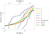 |
Fig. D.1. Cumulative SMG source count. |
Appendix E: Testing the angle recovery algorithm in simulated filaments
To test the success rate in recovering the angle of a filament as traced by SMGs, we created simulated maps of SMGs distributed within filaments of varying widths (0.5 Mpc, 1 Mpc, 1.5 Mpc, and random distribution) and applied the algorithms described in Sect. 5.3. Specifically, for each quasar pair field and filament width, we randomly sampled fluxes between the minimum and maximum detected flux using the normalized source model (Table 2) multiplied by the completeness (Fig. 3) as probability distribution. We then randomly chose a source position in the filament and only kept the simulated SMG if the position fell within the detectable area of the respective flux, until reaching the same source number as in the SMG candidate catalog for the field. Analogously to Sect. 5.3, we calculated αrms and αinertia in the resulting mock map and repeated the process 500 times for every filament width and the random source distributions. The resulting angle probability densities for a stack of all fields is shown in Fig. E.1. While a two-sample Kolmogorov-Smirnov test between the different angles from filaments and the respective random distributions returns p-values below the data type precision, it becomes apparent that αRMS is more successful in recovering the injection angle of zero degrees: the angle distribution of αRMS for the thickest filament has a standard deviation of 20°, while the standard deviation of the distribution for αinertia is 37°.
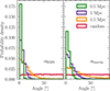 |
Fig. E.1. Absolute recovered angle αRMS (left panel) and αinertia (right panel) for the three tested filament widths 0.5 Mpc, 1 Mpc, and 1.5 Mpc, oriented at an angle of zero degrees, as well as random source distributions. |
All Tables
Information on the quasar pair at the center of the nine observed fields, the coordinates of the pointing and observing conditions.
Parameters of the Schechter functions reproducing the observed source counts, galaxy overdensities calculated from the models, and angle direction of the overdensities.
Quasar coordinates, magnitudes, and submillimeter flux detections above 3σ within 6″ of the quasars. For non-detections, the forced flux at the quasar coordinates is reported and marked with an asterisk.
All Figures
|
Fig. 1. Magnitude and projected distance of the quasar pairs presented in this work (squares) and found in catalogs (circles). The points are color-coded by redshift. |
| In the text | |
|
Fig. 2. S/N maps at 850 μm. The position of the brighter (fainter) quasar is indicated by a black (brown) star. Identified catalog SMGs are marked by black circles with the same size as the effective beam FWHM of 14.6″. The gray dashed line indicates the edge of the effective area (2.5 × the central rms). Sources inconsistent with the expected SMG SED at the quasar redshift are marked with gray rectangles. |
| In the text | |
|
Fig. 3. Completeness percentage of the source extraction as a function of injected source flux in the 450 μm band (left) and the 850 μm band (right). |
| In the text | |
|
Fig. 4. Differential number counts at 850 μm in the data (green points), underlying source model of the quasar pair fields (blue), and 1σ spread of the differential number counts from 500 realizations of the source model (yellow shaded area). For comparison, we show the fiducial field model (black dashed) with its 1σ spread in 500 realizations (gray shaded area). We report the overdensity factor δcumul for each field in the panels. |
| In the text | |
|
Fig. 5. Cumulative SFR of the quasar pair fields compared to the ten protocluster zoom-in simulations of FOREVER22 at z = 3 (Yajima et al. 2022), the 32 most massive halos from Magneticum at z = 2.79 (Remus et al. 2023; Dolag et al. 2025), and known protoclusters from the literature (Wang et al. 2025 and references therein). The dotted line shows the cumulative SFR of the mean blank field in FOREVER22 (Yajima et al. 2022). |
| In the text | |
|
Fig. 6. Cumulative molecular gas mass Mgas of the quasar pair fields compared to the molecular gas mass in the 32 most massive halos in Magneticum at z = 2.79 (Remus et al. 2023; Dolag et al. 2025), estimated from the star-forming gas. |
| In the text | |
|
Fig. 7. SFRD in the central 1 Mpc (SFRDcen) and from the source model of the full field (SFRDint) for quasar pairs, ELANe (Nowotka et al. 2022; Arrigoni Battaia et al. 2023), and single quasars (Arrigoni Battaia et al. 2023), compared to values reported for known protoclusters (Clements et al. 2014; Dannerbauer et al. 2014; Kato et al. 2016) and simulation predictions from FOREVER22 (PCR0; Yajima et al. 2022) and Magneticum Box2b (the most massive halo; Remus et al. 2023), both integrated within the central 1 Mpc (SFRDcen) and 3 Mpc (SFRDint). The solid black line shows the mean cosmic SFRD (Madau & Dickinson 2014); the solid gray lines are the mean cosmic SFRD scaled up by a factor of 100, 1000, and 10 000, respectively; the beige line shows the SFRD for blank field SMGs (Dudzevičiūtė et al. 2020); the dash-dotted line shows the simulation prediction for SFRD within protoclusters by Rennehan (2024); and the dotted line is the SFRD in the Magneticum mean field (Dolag et al. 2025). |
| In the text | |
|
Fig. 8. Direction of the overdensity calculated from the eigenvalue and the minimized rms, as well as the line connecting the quasar pair and the semimajor axis of the nebula, if available. All catalog sources of the fields are plotted; the size and color of the points indicate the weight according to catalog completeness at the flux of the SMG (i.e., within one field; larger and brighter points correspond to higher fluxes). |
| In the text | |
|
Fig. 9. Histogram of the angle difference between semimajor axis of the nebula and direction of the megaparsec-scale SMG distribution αRMS, color-coded by the number of quasars in the center of the field. The angles are compiled from Arrigoni Battaia et al. (2023), Herwig et al. (2024), and Table 2, and are restricted to the range [0° ,90°). The median angle offset of 25° (46°) for single (multiple) quasar fields is marked by the vertical black (gray) line. |
| In the text | |
|
Fig. D.1. Cumulative SMG source count. |
| In the text | |
|
Fig. E.1. Absolute recovered angle αRMS (left panel) and αinertia (right panel) for the three tested filament widths 0.5 Mpc, 1 Mpc, and 1.5 Mpc, oriented at an angle of zero degrees, as well as random source distributions. |
| In the text | |
Current usage metrics show cumulative count of Article Views (full-text article views including HTML views, PDF and ePub downloads, according to the available data) and Abstracts Views on Vision4Press platform.
Data correspond to usage on the plateform after 2015. The current usage metrics is available 48-96 hours after online publication and is updated daily on week days.
Initial download of the metrics may take a while.